Trend Drawing + OB Signal (MTF) [ASCII]Script Description: Advanced Multi-Timeframe Trend Lines & OB/OS Signal
Overview
This advanced Pine Script indicator is designed to identify and project key support and resistance levels using pivot-based trend lines across multiple timeframes. It combines this powerful trend analysis with a sophisticated Overbought/Oversold (OB/OS) detection system using CCI and Bollinger Bands, providing clear trading signals with integrated alert functionality.
Key Features
1. Multi-Timeframe Trend Lines
Automated Pivot Detection: Automatically identifies significant swing highs and lows based on user-defined left/right bar parameters
Smart Timeframe Adaptation: Uses different sensitivity settings for each timeframe (15min to 1Week) for optimal pivot detection
Dynamic Line Projection: Draws trend lines connecting the two most recent pivots and extends them forward
Flexible Source Selection: Choose between Close price, Wick extremes, or Auto mode (Auto uses Wick for higher timeframes, Close for lower timeframes)
2. Advanced OB/OS Detection System
Dual Indicator Confirmation: Combines CCI momentum and Bollinger Band position for reliable signals
Customizable Parameters: Adjustable CCI length, OB/OS thresholds, and Bollinger Band settings
Bar Confirmation Option: Optional wait-for-close confirmation to avoid false signals
Visual Markers: Clear triangle markers above/below bars for quick signal identification
3. Timeframe Support
Available Timeframes: 15min, 30min, 1h, 2h, 4h, 8h, 12h, 1D, 1W
Independent Settings: Custom left/right bar parameters for each timeframe
Automatic Adaptation: Script automatically applies the correct settings for your current chart timeframe
Input Parameters
Trend Lines Configuration
Left/Right Bars: Defines the pivot detection sensitivity for each timeframe
Line Length: Controls how far trend lines extend into the future
Line Source: Choose between Close, Wick, or Auto selection
Colors: Customizable support/resistance line colors
OB/OS Signal Settings
CCI Parameters: Length and OB/OS thresholds
Bollinger Bands: Length and multiplier for band width
Plot Options: Toggle OB markers and bar confirmation
Signal Logic
OB UP Signal (Short Bias)
Conditions: CCI ≥ OB threshold AND Close ≥ Upper Bollinger Band
Marker: Red triangle down above bar
Alert Direction: SHORT
OB DOWN Signal (Long Bias)
Conditions: CCI ≤ OS threshold AND Close ≤ Lower Bollinger Band
Marker: Green triangle up below bar
Alert Direction: LONG
Alert System
The script includes pre-formatted JSON alerts for external integration:
Structured data format with symbol, timeframe, direction, and signal type
Secret key for authentication (replace "MY_SECRET" with your actual key)
Compatible with webhook services and custom alert handlers
Usage Tips
Timeframe Selection: Use higher timeframes (4H-Daily) for major levels, lower timeframes for precise entries
Parameter Tuning: Adjust left/right bars based on market volatility - increase for smoother trends, decrease for more reactive lines
Confirmation: Combine trend line breaks with OB/OS signals for high-probability setups
Risk Management: Always use proper stop losses - trend lines indicate potential areas, not guaranteed reversals
Technical Notes
Built with Pine Script v6
Maximum 200 lines/labels to maintain performance
Works on all asset types (forex, stocks, crypto)
Optimized for real-time and historical analysis
This script provides institutional-grade trend analysis with retail-friendly signals, making complex multi-timeframe analysis accessible to traders of all experience levels.
This description covers all the technical aspects while being accessible for users.
Cari skrip untuk "CCI"

Universal Valuation ~ GForge
🎯 Universal Valuation - GForge
Overview:
The Universal Valuation indicator is a sophisticated technical analysis tool that combines 14 different technical indicators into a single, normalized composite Z-score. This revolutionary approach provides traders and investors with a comprehensive view of an asset's relative valuation state, helping identify potential overvalued and undervalued conditions across any market, any timeframe .
🌟 Key Features:
Multi-Indicator Fusion: Combines RSI, CCI, Bollinger Bands, Price Analysis, Chande Momentum, Disparity Index, Hurst Exponent, IMI, TEMA, VWAP, Intraday Momentum, and advanced Risk Ratios (Sharpe, Sortino, Omega)
Universal Compatibility: Works seamlessly across stocks, forex, crypto, commodities, indices, and any tradeable asset
Multi-Timeframe Support: Optimized for all timeframes from 1-minute scalping to monthly long-term analysis
Professional Visualization: 9 stunning color themes with gradient effects and customizable styling
Comprehensive Dashboard: Real-time table displaying individual indicator scores and overall valuation phase
Smart Alert System: Built-in notifications for extreme valuation conditions
Z-Score Normalization: All indicators standardized for consistent comparison and interpretation
🔬 Technical Methodology:
The indicator employs advanced statistical normalization using Z-scores to transform disparate technical indicators into a unified measurement system. This revolutionary approach solves the fundamental problem of combining indicators with different scales and ranges.
1H MNT
Z-Score Normalization Process:
Raw Calculation: Each indicator is first calculated using its traditional formula (RSI 0-100, CCI unlimited range, etc.)
Statistical Analysis: For each indicator, the system calculates a rolling mean and standard deviation over a customizable lookback period
Z-Score Conversion: Current reading is converted using: Z = (Current Value - Rolling Mean) / Rolling Standard Deviation
Standardization: All Z-scores are clamped between -5 and +5 to prevent extreme outliers from dominating the composite
Democratic Weighting: Each normalized indicator contributes equally to the final composite score
Composite Calculation: Final score = Sum of all active Z-scores / Number of active indicators
Why Z-Scores Make It Universal:
Z-scores transform any indicator reading into "how many standard deviations away from normal this reading is." This means:
• An RSI of 85 on a volatile crypto might have the same Z-score as an RSI of 75 on a stable stock
• A CCI reading of +200 in a trending market might be less extreme than +100 in a ranging market
• Price movements are automatically adjusted for each asset's historical volatility
• Different timeframes are automatically normalized for their typical volatility patterns
This mathematical approach ensures the indicator adapts to any asset's unique characteristics and market conditions.
📊 Detailed Component Analysis:
Technical Indicators:
RSI (Relative Strength Index):
Calculates momentum by comparing recent gains to recent losses over a customizable period (default 21). Values above 70 traditionally indicate overbought conditions, while values below 30 suggest oversold conditions. The Universal Valuation converts these raw RSI values into Z-scores, providing a normalized view of how extreme current RSI readings are compared to historical patterns.
CCI (Commodity Channel Index):
Measures the current price level relative to an average price level over a given period (default 30). CCI compares the typical price (high+low+close)/3 to its simple moving average and divides by the mean absolute deviation. Values above +100 or below -100 indicate price extremes. Our Z-score normalization helps identify when CCI readings are statistically significant.
Bollinger Bands Position:
Calculates where the current price sits within the Bollinger Bands envelope. A value of +1 means price is at the upper band, -1 at the lower band, and 0 at the middle (SMA). This component measures price deviation from the mean in standard deviation units, making it naturally statistical. The Z-score normalization reveals when band position readings are historically extreme.
Price Z-Score:
Direct statistical measurement of how far the current price deviates from its historical mean in standard deviation units. This is the purest form of valuation measurement, showing whether an asset is trading at statistically significant levels relative to its historical price range.
Momentum Indicators:
Chande Momentum Oscillator (CMO):
Unlike RSI, CMO uses the sum of gains and losses rather than averages, making it more sensitive to recent price changes. It calculates (sum of gains - sum of losses) / (sum of gains + sum of losses) × 100. Values range from -100 to +100. The Z-score normalization helps identify when momentum readings are unusually extreme.
Disparity Index:
Measures the percentage difference between current price and its simple moving average: (Price - SMA) / SMA × 100. This shows how far price has deviated from its average, with positive values indicating price above average and negative values below. Z-score normalization reveals when these deviations are statistically significant.
Intraday Momentum Index (IMI):
Similar to RSI but uses intraday price movements instead of closing prices. It compares gains and losses within each session (close vs open) rather than session-to-session changes. This captures intraday sentiment and momentum that closing-based indicators might miss. Particularly useful for detecting intraday reversal patterns.
Intraday Momentum:
Simple but effective measurement of daily price movement: (Close - Open) / Open × 100. This shows the percentage gain or loss within each trading session. When Z-score normalized, it reveals when intraday movements are historically extreme, often indicating climax buying or selling conditions.
Advanced Indicators:
TEMA (Triple Exponential Moving Average):
A sophisticated moving average that applies exponential smoothing three times to reduce lag while maintaining responsiveness. TEMA = 3×EMA₁ - 3×EMA₂ + EMA₃, where each EMA is applied to the previous result. The Z-score of TEMA helps identify when price has moved significantly away from this responsive trend line.
VWAP (Volume Weighted Average Price):
Calculates the average price weighted by volume, giving more importance to prices where more volume occurred. VWAP = Σ(Price × Volume) / Σ(Volume). This represents the "fair value" based on actual trading activity. Z-score normalization shows when current VWAP is statistically extreme relative to historical VWAP levels.
Hurst Exponent:
Advanced mathematical concept measuring market efficiency and trend persistence. Values near 0.5 indicate random walk (efficient market), above 0.5 suggest trending behavior, and below 0.5 indicate mean-reverting markets. The indicator converts this to an oscillator: (Hurst - 0.5) × 100, then applies Z-score normalization to identify extreme efficiency/inefficiency periods.
Risk Ratios:
Sharpe Ratio:
Classic risk-adjusted return measure: (Return - Risk-free Rate) / Standard Deviation of Returns. Higher values indicate better risk-adjusted performance. The Z-score normalization reveals when current risk-adjusted returns are historically high or low, helping identify periods of exceptional or poor risk-adjusted performance.
Sortino Ratio:
Improvement over Sharpe ratio that only penalizes downside volatility: (Return - Risk-free Rate) / Downside Deviation. This gives a more accurate picture of risk-adjusted returns since upside volatility isn't necessarily bad. Z-score normalization helps identify when downside risk-adjusted returns reach extreme levels.
Omega Ratio:
Sophisticated risk measure that considers the probability-weighted ratio of gains versus losses above a threshold: Σ(Gains above threshold) / Σ(Losses below threshold). Values above 1.0 indicate positive expected returns above the threshold. Z-score normalization reveals when probability-weighted risk/reward ratios reach historically significant levels.
🎨 Valuation Phases:
The composite Z-score translates into clear valuation phases:
🔵 Extremely Undervalued: Z-Score ≤ -2.0 (Rare buying opportunities)
🟦 Strongly Undervalued: Z-Score ≤ -1.3 (Strong buying signals)
🟨 Moderately Undervalued: Z-Score ≤ -0.65 (Potential value plays)
⚪ Fairly Valued: Z-Score -0.65 to 0.5 (Neutral territory)
🟨 Slightly Overvalued: Z-Score 0.5 to 1.2 (Caution advised)
🟧 Moderately Overvalued: Z-Score 1.2 to 2.0 (Consider profit-taking)
🔴 Strongly Overvalued: Z-Score > 2.0 (High risk, potential sell signals)
12H GOLD
🌍 Universal Application:
Why "Universal"?
Timeframe Independent: Statistical normalization adapts to any timeframe's volatility characteristics
Market Neutral: Works across different market conditions (trending, ranging, volatile, calm)
Configurable Components: Enable/disable specific indicators based on asset type and market conditions
Adaptive Parameters: All lookback periods are customizable for different trading styles
💡 Optimal Use Cases:
Swing Trading: Identify intermediate-term reversal points
Position Trading: Long-term value assessment for portfolio allocation
Day Trading: Intraday extreme condition alerts
Risk Management: Position sizing based on valuation extremes
Multi-Asset Analysis: Compare relative value across different instruments
Market Timing: Entry and exit point optimization
⚙️ Customization Options:
Component Selection: Enable/disable any of the 14 indicators
Lookback Periods: Adjust Z-score calculation periods for each component
Visual Themes: 9 professional color schemes plus custom colors
Alert Thresholds: Configurable extreme condition notifications
Dashboard Display: Toggle individual component visibility
Background Highlighting: Visual emphasis for extreme conditions
🎯 Interpretation Guide:
For Long Positions:
• Look for Z-scores below -1.3 for entry opportunities
• Consider profit-taking when Z-scores exceed +1.2
• Use extreme readings (< -2.0) for high-conviction entries
For Short Positions:
• Look for Z-scores above +2.0 for entry opportunities
• Cover positions when Z-scores fall below +0.5
• Avoid shorting during extreme undervaluation (< -1.3)
For Risk Management:
• Reduce position sizes during overvalued conditions
• Increase allocation during undervalued periods
• Use neutral zones (±0.5) for position adjustments
🔔 Alert System:
Built-in alerts notify you when:
Composite score enters/exits strong overvalued territory (±2.0)
Composite score enters/exits strong undervalued territory (±1.3)
Extreme conditions are reached (±2.5 for overvalued, -2.0 for undervalued)
Neutral crossovers occur (useful for trend changes)
📈 Performance Optimization:
The indicator includes several performance optimizations:
Efficient calculation methods to minimize processing load
Clamped Z-scores to prevent extreme outliers
Optimized table rendering for smooth operation
🎨 Visual Elements:
Main Plot: Composite Z-score line with dynamic gradient coloring
Zone Fills: Visual bands showing valuation regions
Reference Lines: Key threshold levels clearly marked
Background Highlighting: Extreme condition emphasis
Dashboard Table: Comprehensive component breakdown
Bar Coloring: Optional candlestick coloring based on valuation
🔧 Technical Requirements:
Requires sufficient historical data for accurate Z-score calculations
Recommended minimum: 300+ bars for optimal performance
Works on all TradingView subscription levels
📚 Educational Value:
This indicator serves as an excellent educational tool for:
Understanding statistical normalization in trading
Learning how multiple indicators can be combined effectively
Studying market valuation concepts across different assets
Developing a systematic approach to market analysis
⚠️ Important Notes:
The indicator works best with sufficient historical data
Consider market context and fundamental factors alongside technical signals
Backtest thoroughly before implementing in live trading
Adjust parameters based on specific asset characteristics and trading timeframe
Use in conjunction with other analysis methods for best results
---
⚠️ DISCLAIMER:
This indicator is provided for educational and informational purposes only and should not be considered as financial advice, investment advice, trading advice, or any other type of advice.
The Universal Valuation indicator is a technical analysis tool that provides statistical information about price movements and market conditions. It does not guarantee profits or predict future market movements with certainty.
---
Developed with precision for the TradingView community ~ GForge

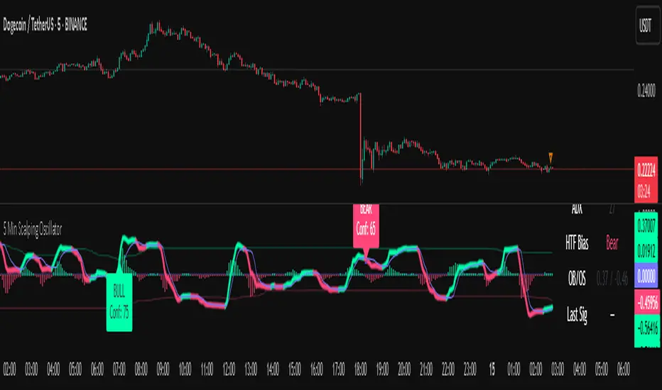
5 Min Scalping Oscillator### Overview
The 5 Min Scalping Oscillator is a custom oscillator designed to provide traders with a unified momentum signal by fusing normalized versions of the Relative Strength Index (RSI), Stochastic RSI, and Commodity Channel Index (CCI). This combination creates a more balanced view of market momentum, overbought/oversold conditions, and potential reversals, while incorporating adaptive smoothing, dynamic thresholds, and market condition filters to reduce noise and false signals. Unlike standalone oscillators, the 5 Min Scalping Oscillator adapts to trending or sideways regimes, volatility levels, and higher timeframe biases, making it particularly suited for short-term charts like 5-minute timeframes where quick, filtered signals are valuable.
### Purpose and Originality of the Fusion
Traditional oscillators like RSI measure momentum but can lag in volatile markets; Stochastic RSI adds sensitivity to RSI extremes but often generates excessive noise; and CCI identifies cyclical deviations but may overreact to minor price swings. The 5 Min Scalping Oscillator addresses these limitations by weighting and blending their normalized outputs (RSI at 45%, Stochastic RSI at 35%, and CCI at 20%) into a single raw oscillator value. This weighted fusion creates a hybrid signal that balances lag reduction with noise filtering, resulting in a more robust indicator for identifying reversal opportunities.
The originality lies in extending this fusion with:
- **Adaptive Smoothing via KAMA (Kaufman's Adaptive Moving Average):** Adjusts responsiveness based on market efficiency, speeding up in trends and slowing in ranges—unlike fixed EMAs, this helps preserve signal integrity without over-smoothing.
- **Dynamic Overbought/Oversold Thresholds:** Calculated using rolling percentiles over a user-defined lookback (default 200+ periods), these levels adapt to recent oscillator behavior rather than relying on static values like 70/30, making the indicator more responsive to asset-specific volatility.
- **Multi-Factor Filters:** Integrates ADX for trend detection, ATR percentiles for volatility confirmation, and optional higher timeframe RSI bias to ensure signals align with broader market context. This layered approach reduces false positives (e.g., ignoring low-volatility crossovers) and adds a confidence score based on filter alignment, which is not typically found in simple mashups.
This design justifies the combination: it's not a mere overlay of indicators but a purposeful integration that enhances usefulness by providing context-aware signals, helping traders avoid common pitfalls like trading against the trend or in low-volatility chop. The result is an original tool that performs better in diverse conditions, especially on 5-minute charts for intraday trading, where rapid adaptations are key.
### How It Works
The 5 Min Scalping Oscillator processes price data through these steps:
1. **Normalization and Fusion:**
- RSI (default length 10) is normalized to a -1 to +1 scale using a tanh transformation for bounded output.
- Stochastic RSI (default length 14) is derived from RSI highs/lows and scaled similarly.
- CCI (default length 14) is tanh-normalized to align with the others.
- These are weighted and summed into a raw value, emphasizing RSI for core momentum while using Stochastic RSI for edge sensitivity and CCI for cycle detection.
2. **Smoothing and Signal Line:**
- The raw value is smoothed (default KAMA with fast/slow periods 2/30 and efficiency length 10) to reduce whipsaws.
- A shorter signal line (half the smoothing length) is added for crossover detections.
3. **Filters and Enhancements:**
- **Trend Regime:** ADX (default length 14, threshold 20) classifies markets as trending (ADX > threshold) or sideways, allowing signals in both but prioritizing alignment.
- **Volatility Check:** ATR (default length 14) percentile (default 85%) ensures signals only trigger in above-average volatility, filtering out flat markets.
- **Higher Timeframe Bias:** Optional RSI (default length 14 on 60-minute timeframe) provides bull/neutral/bear bias (above 55, 45-55, below 45), requiring signal alignment (e.g., bullish signals only if bias is neutral or bull).
- **Dynamic Levels:** Percentiles (default OB 85%, OS 15%) over recent oscillator values set adaptive overbought/oversold lines.
4. **Signal Generation:**
- Bullish (B) signals on upward crossovers of the smoothed line over the signal line, filtered by conditions.
- Bearish (S) signals on downward crossunders.
- Each signal includes a confidence score (0-100) based on factors like trend alignment (25 points), volatility (15 points), and bias (20 points if strong, 10 if neutral).
The output includes a glowing oscillator line, histogram for divergence spotting, dynamic levels, shapes/labels for signals, and a dashboard table summarizing regime, ADX, bias, levels, and last signal.
### How to Use It
This indicator is easy to apply and interpret, even for beginners:
- **Adding to Chart:** Apply the 5 Min Scalping Oscillator to a clean chart (no other indicators unless explained). It's non-overlay, so it appears in a separate pane. For 5-minute timeframes, keep defaults or tweak lengths shorter for faster response (e.g., RSI 8-12).
- **Interpreting Signals:**
- Look for green upward triangles labeled "B" (bullish) at the bottom for potential entry opportunities in uptrends or reversals.
- Red downward triangles labeled "S" (bearish) at the top signal potential exits or shorts.
- Higher confidence scores (e.g., 70+) indicate stronger alignment—use these for priority trades.
- Watch the histogram for divergences (e.g., price higher highs but histogram lower highs suggest weakening momentum).
- Dynamic OB (green line) and OS (red line) help gauge extremes; signals near these are more reliable.
- **Dashboard:** At the bottom-right, it shows real-time info like "Trending" or "Sideways" regime, ADX value, HTF bias (Bull/Neutral/Bear), OB/OS levels, and last signal—use this for quick context.
- **Customization:** Adjust inputs via the settings panel:
- Toggle KAMA for adaptive vs. EMA smoothing.
- Set HTF to "60" for 1-hour bias on 5-min charts.
- Increase ADX threshold to 25 for stricter trend filtering.
- **Best Practices:** Combine with price action (e.g., support/resistance) or volume for confirmation. On 5-min charts, pair with a 1-hour HTF for intraday scalping. Always use stop-losses and risk no more than 1-2% per trade.
### Default Settings Explanation
Defaults are optimized for 5-minute charts on volatile assets like stocks or forex:
- RSI/Stoch/CCI lengths (10/14/14): Shorter for quick momentum capture.
- Signal smoothing (5): Responsive without excessive lag.
- ADX threshold (20): Balances trend detection.
- ATR percentile (0.85): Filters ~15% of low-vol signals.
- HTF RSI (14 on 60-min): Aligns with hourly trends.
- Percentiles (OB 85%, OS 15%): Adaptive to recent data.
If changing, test on historical data to ensure fit—e.g., longer lengths for less noisy assets.
### Disclaimer
The 5 Min Scalping Oscillator is an educational tool to visualize momentum and does not guarantee profits or predict future performance. All signals are based on historical calculations and should not be used as standalone trading advice. Past results are not indicative of future outcomes. Traders must conduct their own analysis, use proper risk management, and consider market conditions. No claims are made about accuracy, reliability, or performance.
TrendSurfer VF 3.4Questo è il mio Trend Surfer.
I triangoli indicano candele direzionali con vari livelli di volume all'interno da 1 a 10.
Per comodità vengono mostrati solo i livelli da 6 a 10.
Se la candela si trova nei pressi del VWAP ancorato il colore del numero sarà verde, ad indicare un'alta probabilità.
I cerchi invece si basano sull'oscillatore CCI (Commodity Channel Index).
L’indicatore CCI ci permette di osservare se il livello attuale del prezzo è particolarmente al di sopra o al di sotto di una certa media mobile, avente un numero di periodi scelto da noi.
Più la deviazione dal prezzo medio nel breve termine è forte, e maggiormente l’indicatore si allontanerà dallo 0: verso l’alto in caso di uptrend, o verso il basso in caso di downtrend.
Il segnale viene dato quando il valore del CCI supera la linea dello zero.
Il tutto è filtrato con un altro indicatore, il MACD, acronimo di "Moving Average Convergence Divergence", usato per identificare cambiamenti nel momentum del prezzo.
This is my Trend Surfer.
The triangles indicate directional candles with varying volume levels from 1 to 10.
For convenience, only levels 6 to 10 are shown.
If the candle is near the anchored VWAP, the color of the number will be green, indicating a high probability.
The circles, on the other hand, are based on the CCI (Commodity Channel Index) oscillator.
The CCI indicator allows us to observe whether the current price level is significantly above or below a certain moving average, with a number of periods chosen by us.
The greater the deviation from the short-term average price, the further the indicator will deviate from 0: upwards in the case of an uptrend, or downwards in the case of a downtrend.
The signal is given when the CCI value crosses the zero line.
This is all filtered through another indicator, the MACD, which stands for "Moving Average Convergence Divergence," used to identify changes in price momentum.

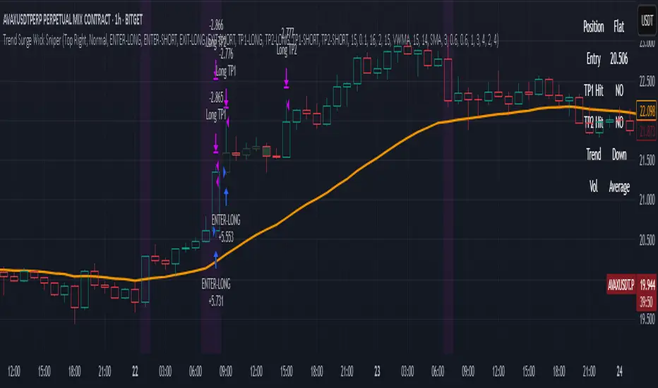
Trend Surge Wick SniperTrend Surge Wick Sniper | Non-Repainting Trend + Momentum Strategy with TP1/TP2 & Dashboard
Trend Surge Wick Sniper is a complete crypto trading strategy designed for high-precision entries, smart exits, and non-repainting execution. It combines trend slope, wick rejection, volume confirmation, and CCI momentum filters into a seamless system that works in real-time conditions — whether you're manual trading or sending alerts to multi-exchange bots.
🧩 System Architecture Overview
This is not just a mashup of indicators — each layer is tightly integrated to filter for confirmed, high-quality setups. Here’s a detailed breakdown:
📈 Trend Logic
1. McGinley Dynamic Baseline
A responsive moving average that adapts to market speed better than EMA or SMA.
Smooths price while staying close to real action, making it ideal for basing alignment or trend context.
2. Gradient Slope Filter (ATR-normalized)
Calculates the difference between current and past McGinley values, divided by ATR for normalization.
If the slope exceeds a configurable threshold, it confirms an active uptrend or downtrend.
Optional loosened sensitivity allows for more frequent but still valid trades.
🚀 Momentum Timing
3. Smoothed CCI (ZLEMA / Hull / VWMA options)
Traditional CCI is enhanced with smoothing for stability.
Signals trades only when momentum is strong and accelerating.
Optional settings let users tune how responsive or smooth they want the CCI behavior to be.
🔒 Entry Filtering & Rejection Logic
4. Wick Trap Detection
Prevents entry during manipulated candles (e.g. stop hunts, wick traps).
Measures wick-to-body ratio against a minimum body size normalized by ATR.
Only trades when the candle shows a clean body and no manipulation.
5. Price Action Filters (Optional)
Long trades require price to break above previous high (or skip this with a toggle).
Short trades require price to break below previous low (or skip this with a toggle).
Ensures you're trading only when price structure confirms the breakout.
6. McGinley Alignment (Optional)
Price must be on the correct side of the McGinley line (above for longs, below for shorts).
Ensures that trades align with baseline trend, preventing early or fading entries.
📊 Volume Logic
7. Volume Spike Detection
Confirms that a real move is underway by requiring volume to exceed a moving average by a user-defined multiplier.
Uses SMA / EMA / VWMA for customizable behavior.
Optional relative volume mode compares volume against typical volume at that same time of day.
8. Volume Trend Filter
Compares fast vs. slow EMA of the volume spike ratio.
Ensures volume is not just spiking, but also increasing overall.
Prevents trades during volume exhaustion or fading participation.
9. Volume Strength Label
Classifies each bar’s volume as: Low, Average, High, or Very High
Shown in the dashboard for context before entries.
🎯 Entry Conditions
An entry occurs when all of the following align:
✅ Trend confirmed via gradient slope
✅ Momentum confirmed via smoothed CCI
✅ No wick trap pattern
✅ Price structure & McGinley alignment (if toggled on)
✅ Volume confirms participation
✅ 1-bar cooldown since last exit
💰 TP1 & TP2 Exit System
TP1 = 50% of position closed using a limit order at a % profit (e.g., 2%)
TP2 = remaining 50% closed at a second profit level (e.g., 4%)
These are set as limit orders at the time of entry and work even on backtest.
Alerts are sent separately for TP1 and TP2 to allow bot handling of staggered exits.
🧠 Trade Logic Controls
✅ process_orders_on_close=true ensures non-repainting behavior
✅ 1-bar cooldown after any exit prevents same-bar reversals
✅ Built-in canEnter condition ensures trades are separated and clean
✅ Alerts use customizable strings for entry/exit/TP1/TP2 — ready for webhook automation
📊 Real-Time On-Chart Dashboard
Toggleable, movable dashboard shows live trading stats:
🔵 Current Position: Long / Short / Flat
🎯 Entry Price
✅ TP1 / TP2 Hit Status
📈 Trend Direction: Up / Down / Flat
🔊 Volume Strength: Low / Average / High / Very High
🎛 Size and corner are adjustable via input settings
⚠️ Designed For:
1H / 4H Crypto Trading
Manual Traders & Webhook-Connected Bots
Scalability across volatile market conditions
Full TradingView backtest compatibility (no repainting / no fake signals)
📌 Notes
You can switch CCI smoothing type, volume MA type, and other filters via the settings panel.
Default TP1/TP2 levels are set to 2% and 4%, but fully customizable.
🛡 Disclaimer
This script is for educational purposes only and not financial advice. Use with backtesting and risk management before live deployment.
Multi Oscillator OB/OS Signals v3 - Scope TestIndicator Description: Multi Oscillator OB/OS Signals
Purpose:
The "Multi Oscillator OB/OS Signals" indicator is a TradingView tool designed to help traders identify potential market extremes and momentum shifts by monitoring four popular oscillators simultaneously: RSI, Stochastic RSI, CCI, and MACD. Instead of displaying these oscillators in separate panes, this indicator plots distinct visual symbols directly onto the main price chart whenever specific predefined conditions (typically related to overbought/oversold levels or line crossovers) are met for each oscillator. This provides a consolidated view of potential signals from these different technical tools.
How It Works:
The indicator calculates the values for each of the four oscillators based on user-defined settings (like length periods and price sources) and then checks for specific signal conditions on every bar:
Relative Strength Index (RSI):
It monitors the standard RSI value.
When the RSI crosses above the user-defined Overbought (OB) level (e.g., 70), it plots an "Overbought" symbol (like a downward triangle) above that price bar.
When the RSI crosses below the user-defined Oversold (OS) level (e.g., 30), it plots an "Oversold" symbol (like an upward triangle) below that price bar.
Stochastic RSI:
This works similarly to RSI but is based on the Stochastic calculation applied to the RSI value itself (specifically, the %K line of the Stoch RSI).
When the Stoch RSI's %K line crosses above its Overbought level (e.g., 80), it plots its designated OB symbol (like a downward arrow) above the bar.
When the %K line crosses below its Oversold level (e.g., 20), it plots its OS symbol (like an upward arrow) below the bar.
Commodity Channel Index (CCI):
It tracks the CCI value.
When the CCI crosses above its Overbought level (e.g., +100), it plots its OB symbol (like a square) above the bar.
When the CCI crosses below its Oversold level (e.g., -100), it plots its OS symbol (like a square) below the bar.
Moving Average Convergence Divergence (MACD):
Unlike the others, MACD signals here are not based on fixed OB/OS levels.
It identifies when the main MACD line crosses above its Signal line. This is considered a bullish crossover and is indicated by a specific symbol (like an upward label) plotted below the price bar.
It also identifies when the MACD line crosses below its Signal line. This is a bearish crossover, indicated by a different symbol (like a downward label) plotted above the price bar.
Visualization:
All these signals appear as small, distinct shapes directly on the price chart at the bar where the condition occurred. The shapes, their colors, and their position (above or below the bar) are predefined for each signal type to allow for quick visual identification. Note: In the current version of the underlying code, the size of these shapes is fixed (e.g., tiny) and not user-adjustable via the settings.
Configuration:
Users can access the indicator's settings to customize:
The calculation parameters (Length periods, smoothing, price source) for each individual oscillator (RSI, Stoch RSI, CCI, MACD).
The specific Overbought and Oversold threshold levels for RSI, Stoch RSI, and CCI.
The colors associated with each type of signal (OB, OS, Bullish Cross, Bearish Cross).
(Limitation Note: While settings exist to toggle the visibility of signals for each oscillator individually, due to a technical workaround in the current code, these toggles may not actively prevent the shapes from plotting if the underlying condition is met.)
Alerts:
The indicator itself does not automatically generate pop-up alerts. However, it creates the necessary "Alert Conditions" within TradingView's alert system. This means users can manually set up alerts for any of the specific signals generated by the indicator (e.g., "RSI Overbought Enter," "MACD Bullish Crossover"). When creating an alert, the user selects this indicator, chooses the desired condition from the list provided by the script, and configures the alert actions.
Intended Use:
This indicator aims to provide traders with convenient visual cues for potential over-extension in price (via OB/OS signals) or shifts in momentum (via MACD crossovers) based on multiple standard oscillators. These signals are often used as potential indicators for:
Identifying areas where a trend might be exhausted and prone to a pullback or reversal.
Confirming signals generated by other analysis methods or trading strategies.
Noting shifts in short-term momentum.
Disclaimer: As with any technical indicator, the signals generated should not be taken as direct buy or sell recommendations. They are best used in conjunction with other forms of analysis (price action, trend analysis, volume, fundamental analysis, etc.) and within the framework of a well-defined trading plan that includes risk management. Market conditions can change, and indicator signals can sometimes be false or misleading.

LiquidFusion SignalPro [CHE] LiquidFusion SignalPro – Indicator Overview
The LiquidFusion SignalPro is a powerful and sophisticated TradingView indicator designed to identify high-quality trade entries and exits. By combining seven unique sub-indicators, it provides comprehensive market analysis, ensuring traders can make informed decisions. This tool is suitable for all market conditions and supports customization to fit individual trading strategies.
Key Components (Sub-Indicators):
1. RPM (Relative Price Momentum):
- Measures cumulative price momentum over a specified period.
- Provides insights into price strength and directional bias.
- Input Customization:
- Source: Data for momentum calculation.
- Period: Length for momentum measurement.
- Resolution: Timeframe for data fetching.
2. BBO (Bull-Bear Oscillator):
- Calculates the strength of bullish or bearish momentum based on price movement and RSI conditions.
- Uses a super-smoothing technique for reliable signals.
- Customizable parameters include the oscillator's period and repainting options.
3. MACD (Moving Average Convergence Divergence):
- A classic momentum indicator for trend direction and strength.
- Provides buy/sell signals based on the crossover of the MACD line and signal line.
- Input Customization:
- Fast/Slow EMA Periods.
- Signal Line Period.
- Resolution and Source Data.
4. RSI (Relative Strength Index):
- Tracks overbought and oversold conditions.
- A key tool to validate trend continuation or reversals.
- Customizable period, resolution, and source.
5. CCI (Commodity Channel Index):
- Measures the deviation of price from its average.
- Useful for identifying cyclical trends.
- Input Customization includes period, resolution, and source.
6. Stochastic Oscillator:
- Indicates momentum by comparing closing prices to a range of highs and lows.
- Includes smoothing factors for %K and %D lines.
- Customizable parameters:
- %K Length and Smoothing.
- Resolution and Repainting Options.
7. Supertrend:
- A trailing stop-and-reverse system for trend-following strategies.
- Excellent for identifying strong trends and potential reversals.
- Inputs include the multiplier factor and period for ATR-like calculations.
Inputs Overview:
The indicator supports extensive customization for each sub-indicator, grouped under intuitive categories:
- Color Settings: Define bullish and bearish plot colors.
- RPM, BBO, MACD, RSI, CCI, Stochastic, and Supertrend Settings: Tailor each sub-indicator's behavior with adjustable parameters.
- UI Options: Toggle features such as bar coloring, indicator names, and plotted candles.
Trade Signals:
- Long Signal:
- All indicators align in a bullish state:
- RPM > 0, MACD > 0, RSI > 50, Stochastic > 50, CCI > 0, BBO > 0, Supertrend below price.
- Plot: Green triangle below the candle.
- Alert: Notifies the trader of a potential long entry.
- Short Signal:
- All indicators align in a bearish state:
- RPM < 0, MACD < 0, RSI < 50, Stochastic < 50, CCI < 0, BBO < 0, Supertrend above price.
- Plot: Red triangle above the candle.
- Alert: Notifies the trader of a potential short entry.
Features:
- Enhanced Visuals: Plots sub-indicator statuses using labels and color-coded shapes for clarity.
- Alerts: Integrated alert conditions for both long and short trades.
- Bar Coloring: Provides overall trend bias with green (bullish), red (bearish), or gray (neutral) bars.
- Customizable Table: Displays the indicator's status in the chart’s top-right corner.
Trading Benefits:
The LiquidFusion SignalPro excels in generating high-quality entries and exits by:
- Reducing noise through multiple indicator alignment.
- Supporting multiple timeframes and resolutions for flexibility.
- Offering customizable inputs for personalized trading strategies.
Use this tool to enhance your market analysis and improve your trading performance.
Disclaimer:
The content provided, including all code and materials, is strictly for educational and informational purposes only. It is not intended as, and should not be interpreted as, financial advice, a recommendation to buy or sell any financial instrument, or an offer of any financial product or service. All strategies, tools, and examples discussed are provided for illustrative purposes to demonstrate coding techniques and the functionality of Pine Script within a trading context.
Any results from strategies or tools provided are hypothetical, and past performance is not indicative of future results. Trading and investing involve high risk, including the potential loss of principal, and may not be suitable for all individuals. Before making any trading decisions, please consult with a qualified financial professional to understand the risks involved.
By using this script, you acknowledge and agree that any trading decisions are made solely at your discretion and risk.
This indicator is inspired by the Super 6x Indicators: RSI, MACD, Stochastic, Loxxer, CCI, and Velocity . A special thanks to Loxx for their relentless effort, creativity, and contributions to the TradingView community, which served as a foundation for this work.
Happy trading and best regards
Chervolino

HMM Regime IndicatorHMM Regime Indicator
Overview:
The HMM Regime Indicator is designed to help traders identify market regimes by analyzing trend strength, momentum, and price deviation. It uses a combination of the Average Directional Index (ADX), Relative Strength Index (RSI), and Commodity Channel Index (CCI) to classify market conditions into three distinct regimes: Bullish, Bearish, and Sideways.
Key Features:
ADX (Average Directional Index): Measures the strength of a trend. A high ADX value indicates a strong trend, while a low value suggests a weak or non-existent trend.
RSI (Relative Strength Index): Identifies overbought or oversold conditions. An RSI above 70 typically indicates overbought conditions, while an RSI below 30 suggests oversold conditions.
CCI (Commodity Channel Index): Evaluates the price deviation from its average. High CCI values indicate that prices are well above their average, while low values suggest prices are below their average.
Regime Detection:
Bullish Regime: Identified when the ADX indicates a strong trend, and both RSI and CCI suggest overbought conditions. This regime is marked with a green background on the chart.
Bearish Regime: Detected when the ADX shows a strong trend, and both RSI and CCI indicate oversold conditions. This regime is highlighted with a red background.
Sideways Regime: Occurs when neither bullish nor bearish conditions are met, suggesting a lack of strong directional movement. This regime is shown with a blue background.
Usage:
This indicator is useful for traders looking to understand the current market environment and adjust their strategies accordingly. By identifying the prevailing market regime, traders can make more informed decisions about entering or exiting trades.
Customization:
Users can adjust the input parameters for ADX, RSI, and CCI to better fit their trading style and the specific asset being analyzed. The default settings are optimized for general use but can be tailored to suit individual preferences.

The Trend SetterThe "Trend Setter" script is a technical indicator that combines several other indicators to identify trends and potential entry points in the market. It is designed to work with various financial markets, including stocks, forex, and futures, and can be used on any timeframe.
The script uses the TTM Squeeze indicator, Bollinger Bands, Keltner Channels, CCI, and Parabolic SAR to identify trends and potential entry points. The TTM Squeeze is a custom indicator that identifies periods of low volatility, while the Bollinger Bands and Keltner Channels are used to identify potential breakouts. The CCI is used to identify potential overbought and oversold conditions, and the Parabolic SAR is used to identify potential trend reversals.
The TTM Squeeze indicator is a combination of Bollinger Bands and Keltner Channels. The indicator creates a "squeeze" when the Bollinger Bands move inside the Keltner Channels. This indicates a period of low volatility and is often followed by a period of increased volatility or a breakout. The script uses this information to identify potential trading opportunities.
The Bollinger Bands are a popular indicator used to identify potential breakouts. They consist of a moving average (the basis) and two standard deviation lines (the upper and lower bands). When the price moves outside the bands, it is considered a potential breakout.
Keltner Channels are similar to Bollinger Bands but are based on the Average True Range (ATR) instead of standard deviation. They consist of an exponential moving average (the basis) and two lines that are offset from the basis by a multiple of the ATR. When the price moves outside the channels, it is considered a potential breakout.
The CCI (Commodity Channel Index) is used to identify potential overbought and oversold conditions. It measures the difference between the typical price (the average of the high, low, and close) and a moving average of the typical price. The result is then divided by a multiple of the mean deviation. When the CCI moves above a certain threshold, it is considered overbought, and when it moves below a certain threshold, it is considered oversold.
The Parabolic SAR (Stop and Reverse) is used to identify potential trend reversals. It consists of a series of dots that appear above or below the price, depending on the direction of the trend. When the price crosses the dots, it is considered a potential reversal.
The script plots arrow shapes on the chart to indicate long and short entry points, and can also generate alerts to notify the user of potential trading opportunities. The script uses the various indicators to determine the potential entry points based on the current market conditions.
Overall, the script is designed to help traders identify potential trading opportunities and make more informed trading decisions. However, as with any trading strategy or indicator, it is important to thoroughly test and validate the approach before using it in a live trading environment. Traders should also consider their risk tolerance and other factors before making any trades based on the indicator.
In assembling the different indicators in this script, there is a specific rationale for each one's inclusion, and how they work together to create a comprehensive trading strategy.
The TTM Squeeze indicator is used as a primary filter to identify periods of low volatility, as these are often followed by high volatility and potential breakouts. Bollinger Bands and Keltner Channels are then used to identify potential breakouts, with the former representing the upper and lower boundaries of price action and the latter representing the average price range. The inclusion of both indicators helps to confirm potential breakouts and provide a more comprehensive view of price action.
The CCI indicator is used as a momentum indicator to confirm potential trend reversals, by identifying overbought and oversold conditions. This is important because while breakouts can be identified using the TTM Squeeze and Bollinger Bands/Keltner Channels, they do not necessarily indicate the direction of the breakout. The CCI helps to confirm whether the price is overbought or oversold, and can indicate potential reversals or continuations of the trend.
Finally, the Parabolic SAR is used as a trend-following indicator to identify potential trend reversals, by placing dots above or below the price depending on the direction of the trend. This helps to identify potential reversal points in the trend and can be used in conjunction with other indicators to confirm potential entry and exit points.
In summary, the combination of these indicators is designed to provide a comprehensive view of the market, identifying periods of low volatility, potential breakouts, momentum changes, and trend reversals. By providing clear entry and exit points, the script aims to help traders make more informed trading decisions and improve their overall trading performance.
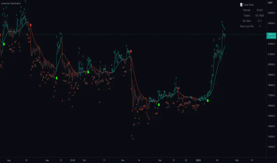
Machine Learning: Lorentzian Classification█ OVERVIEW
A Lorentzian Distance Classifier (LDC) is a Machine Learning classification algorithm capable of categorizing historical data from a multi-dimensional feature space. This indicator demonstrates how Lorentzian Classification can also be used to predict the direction of future price movements when used as the distance metric for a novel implementation of an Approximate Nearest Neighbors (ANN) algorithm.
█ BACKGROUND
In physics, Lorentzian space is perhaps best known for its role in describing the curvature of space-time in Einstein's theory of General Relativity (2). Interestingly, however, this abstract concept from theoretical physics also has tangible real-world applications in trading.
Recently, it was hypothesized that Lorentzian space was also well-suited for analyzing time-series data (4), (5). This hypothesis has been supported by several empirical studies that demonstrate that Lorentzian distance is more robust to outliers and noise than the more commonly used Euclidean distance (1), (3), (6). Furthermore, Lorentzian distance was also shown to outperform dozens of other highly regarded distance metrics, including Manhattan distance, Bhattacharyya similarity, and Cosine similarity (1), (3). Outside of Dynamic Time Warping based approaches, which are unfortunately too computationally intensive for PineScript at this time, the Lorentzian Distance metric consistently scores the highest mean accuracy over a wide variety of time series data sets (1).
Euclidean distance is commonly used as the default distance metric for NN-based search algorithms, but it may not always be the best choice when dealing with financial market data. This is because financial market data can be significantly impacted by proximity to major world events such as FOMC Meetings and Black Swan events. This event-based distortion of market data can be framed as similar to the gravitational warping caused by a massive object on the space-time continuum. For financial markets, the analogous continuum that experiences warping can be referred to as "price-time".
Below is a side-by-side comparison of how neighborhoods of similar historical points appear in three-dimensional Euclidean Space and Lorentzian Space:
This figure demonstrates how Lorentzian space can better accommodate the warping of price-time since the Lorentzian distance function compresses the Euclidean neighborhood in such a way that the new neighborhood distribution in Lorentzian space tends to cluster around each of the major feature axes in addition to the origin itself. This means that, even though some nearest neighbors will be the same regardless of the distance metric used, Lorentzian space will also allow for the consideration of historical points that would otherwise never be considered with a Euclidean distance metric.
Intuitively, the advantage inherent in the Lorentzian distance metric makes sense. For example, it is logical that the price action that occurs in the hours after Chairman Powell finishes delivering a speech would resemble at least some of the previous times when he finished delivering a speech. This may be true regardless of other factors, such as whether or not the market was overbought or oversold at the time or if the macro conditions were more bullish or bearish overall. These historical reference points are extremely valuable for predictive models, yet the Euclidean distance metric would miss these neighbors entirely, often in favor of irrelevant data points from the day before the event. By using Lorentzian distance as a metric, the ML model is instead able to consider the warping of price-time caused by the event and, ultimately, transcend the temporal bias imposed on it by the time series.
For more information on the implementation details of the Approximate Nearest Neighbors (ANN) algorithm used in this indicator, please refer to the detailed comments in the source code.
█ HOW TO USE
Below is an explanatory breakdown of the different parts of this indicator as it appears in the interface:
Below is an explanation of the different settings for this indicator:
General Settings:
Source - This has a default value of "hlc3" and is used to control the input data source.
Neighbors Count - This has a default value of 8, a minimum value of 1, a maximum value of 100, and a step of 1. It is used to control the number of neighbors to consider.
Max Bars Back - This has a default value of 2000.
Feature Count - This has a default value of 5, a minimum value of 2, and a maximum value of 5. It controls the number of features to use for ML predictions.
Color Compression - This has a default value of 1, a minimum value of 1, and a maximum value of 10. It is used to control the compression factor for adjusting the intensity of the color scale.
Show Exits - This has a default value of false. It controls whether to show the exit threshold on the chart.
Use Dynamic Exits - This has a default value of false. It is used to control whether to attempt to let profits ride by dynamically adjusting the exit threshold based on kernel regression.
Feature Engineering Settings:
Note: The Feature Engineering section is for fine-tuning the features used for ML predictions. The default values are optimized for the 4H to 12H timeframes for most charts, but they should also work reasonably well for other timeframes. By default, the model can support features that accept two parameters (Parameter A and Parameter B, respectively). Even though there are only 4 features provided by default, the same feature with different settings counts as two separate features. If the feature only accepts one parameter, then the second parameter will default to EMA-based smoothing with a default value of 1. These features represent the most effective combination I have encountered in my testing, but additional features may be added as additional options in the future.
Feature 1 - This has a default value of "RSI" and options are: "RSI", "WT", "CCI", "ADX".
Feature 2 - This has a default value of "WT" and options are: "RSI", "WT", "CCI", "ADX".
Feature 3 - This has a default value of "CCI" and options are: "RSI", "WT", "CCI", "ADX".
Feature 4 - This has a default value of "ADX" and options are: "RSI", "WT", "CCI", "ADX".
Feature 5 - This has a default value of "RSI" and options are: "RSI", "WT", "CCI", "ADX".
Filters Settings:
Use Volatility Filter - This has a default value of true. It is used to control whether to use the volatility filter.
Use Regime Filter - This has a default value of true. It is used to control whether to use the trend detection filter.
Use ADX Filter - This has a default value of false. It is used to control whether to use the ADX filter.
Regime Threshold - This has a default value of -0.1, a minimum value of -10, a maximum value of 10, and a step of 0.1. It is used to control the Regime Detection filter for detecting Trending/Ranging markets.
ADX Threshold - This has a default value of 20, a minimum value of 0, a maximum value of 100, and a step of 1. It is used to control the threshold for detecting Trending/Ranging markets.
Kernel Regression Settings:
Trade with Kernel - This has a default value of true. It is used to control whether to trade with the kernel.
Show Kernel Estimate - This has a default value of true. It is used to control whether to show the kernel estimate.
Lookback Window - This has a default value of 8 and a minimum value of 3. It is used to control the number of bars used for the estimation. Recommended range: 3-50
Relative Weighting - This has a default value of 8 and a step size of 0.25. It is used to control the relative weighting of time frames. Recommended range: 0.25-25
Start Regression at Bar - This has a default value of 25. It is used to control the bar index on which to start regression. Recommended range: 0-25
Display Settings:
Show Bar Colors - This has a default value of true. It is used to control whether to show the bar colors.
Show Bar Prediction Values - This has a default value of true. It controls whether to show the ML model's evaluation of each bar as an integer.
Use ATR Offset - This has a default value of false. It controls whether to use the ATR offset instead of the bar prediction offset.
Bar Prediction Offset - This has a default value of 0 and a minimum value of 0. It is used to control the offset of the bar predictions as a percentage from the bar high or close.
Backtesting Settings:
Show Backtest Results - This has a default value of true. It is used to control whether to display the win rate of the given configuration.
█ WORKS CITED
(1) R. Giusti and G. E. A. P. A. Batista, "An Empirical Comparison of Dissimilarity Measures for Time Series Classification," 2013 Brazilian Conference on Intelligent Systems, Oct. 2013, DOI: 10.1109/bracis.2013.22.
(2) Y. Kerimbekov, H. Ş. Bilge, and H. H. Uğurlu, "The use of Lorentzian distance metric in classification problems," Pattern Recognition Letters, vol. 84, 170–176, Dec. 2016, DOI: 10.1016/j.patrec.2016.09.006.
(3) A. Bagnall, A. Bostrom, J. Large, and J. Lines, "The Great Time Series Classification Bake Off: An Experimental Evaluation of Recently Proposed Algorithms." ResearchGate, Feb. 04, 2016.
(4) H. Ş. Bilge, Yerzhan Kerimbekov, and Hasan Hüseyin Uğurlu, "A new classification method by using Lorentzian distance metric," ResearchGate, Sep. 02, 2015.
(5) Y. Kerimbekov and H. Şakir Bilge, "Lorentzian Distance Classifier for Multiple Features," Proceedings of the 6th International Conference on Pattern Recognition Applications and Methods, 2017, DOI: 10.5220/0006197004930501.
(6) V. Surya Prasath et al., "Effects of Distance Measure Choice on KNN Classifier Performance - A Review." .
█ ACKNOWLEDGEMENTS
@veryfid - For many invaluable insights, discussions, and advice that helped to shape this project.
@capissimo - For open sourcing his interesting ideas regarding various KNN implementations in PineScript, several of which helped inspire my original undertaking of this project.
@RikkiTavi - For many invaluable physics-related conversations and for his helping me develop a mechanism for visualizing various distance algorithms in 3D using JavaScript
@jlaurel - For invaluable literature recommendations that helped me to understand the underlying subject matter of this project.
@annutara - For help in beta-testing this indicator and for sharing many helpful ideas and insights early on in its development.
@jasontaylor7 - For helping to beta-test this indicator and for many helpful conversations that helped to shape my backtesting workflow
@meddymarkusvanhala - For helping to beta-test this indicator
@dlbnext - For incredibly detailed backtesting testing of this indicator and for sharing numerous ideas on how the user experience could be improved.
Digital Kahler Stochastic [Loxx]Digital Kahler Stochastic is a Digital Kahler filtered Stochastic. This modification significantly reduces noise.
What is Digital Kahler?
From Philipp Kahler's article for www.traders-mag.com, August 2008. "A Classic Indicator in a New Suit: Digital Stochastic"
Digital Indicators
Whenever you study the development of trading systems in particular, you will be struck in an extremely unpleasant way by the seemingly unmotivated indentations and changes in direction of each indicator. An experienced trader can recognise many false signals of the indicator on the basis of his solid background; a stupid trading system usually falls into any trap offered by the unclear indicator course. This is what motivated me to improve even further this and other indicators with the help of a relatively simple procedure. The goal of this development is to be able to use this indicator in a trading system with as few additional conditions as possible. Discretionary traders will likewise be happy about this clear course, which is not nerve-racking and makes concentrating on the essential elements of trading possible.
How Is It Done?
The digital stochastic is a child of the original indicator. We owe a debt of gratitude to George Lane for his idea to design an indicator which describes the position of the current price within the high-low range of the historical price movement. My contribution to this indicator is the changed pattern which improves the quality of the signal without generating too long delays in giving signals. The trick used to generate this “digital” behavior of the indicator. It can be used with most oscillators like RSI or CCI .
First of all, the original is looked at. The indicator always moves between 0 and 100. The precise position of the indicator or its course relative to the trigger line are of no interest to me, I would just like to know whether the indicator is quoted below or above the value 50. This is tantamount to the question of whether the market is just trading above or below the middle of the high-low range of the past few days. If the market trades in the upper half of its high-low range, then the digital stochastic is given the value 1; if the original stochastic is below 50, then the value –1 is given. This leads to a sequence of 1/-1 values – the digital core of the new indicator. These values are subsequently smoothed by means of a short exponential moving average . This way minor false signals are eliminated and the indicator is given its typical form.
Calculation
The calculation is simple
Step1: create the CCI
Step 2: Use CCI as Fast MA and smoothed CCI as Slow MA
Step 3: Multiple the Slow and Fast MAs by their respective input ratios, and then divide by their sum. if the result is greater than 0, then the result is 1, if it's less than 0 then the result is -1, then chart the data
if ((slowr * slow_k + fastr * fast_k) / (fastr + slowr) > 50.0)
temp := 1
if ((slowr * slow_k + fastr * fast_k) / (fastr + slowr) < 50.0)
temp := -1
Step 4: Profit
Other implementations of Digital Kahler
This is to better understand the process the DK process and it's result, and furthermore, I'm linking these because for many in the Forex community, they see DK filtered indicators as the best implementations of standard indicators.
Digital Kahler MACD
VHF-Adaptive, Digital Kahler Variety RSI w/ Dynamic Zones
Digital Kahler CCI
Included:
Bar coloring
Signals
Alerts
Loxx's Expanded Source Types
Loxx's Moving Averages
ExpertToken Buy/Sell SignalExpertToken Buy/Sell Signal เป็นอินดิเคเตอร์ที่สามารถบอกสัญญาณการซื้อขาย และบอกแนวโน้มของราคาได้
หลักการทำงาน
สัญญาณ Buy/Sell ถูกกำหนดโดยการใช่ CCI วัดโมเมนตัมการซื้อขาย หาก CCI ส่งสัญญาณว่าแรงขายเยอะเกินไป และมีแนวโน้มราคาจะกลับตัวสูงขึ้น ก็จะส่งสัญญาณ Buy แต่หาก CCI ส่งสัญญาณว่าแรงซื้อเยอะเกินไป และมีแนวโน้มราคาจะกลับตัวต่ำลง ก็จะส่งสัญญาณ Buy
เส้นสีน้ำเงินเป็นเส้น EMA 200 ไว้ใช้บอกแนวโน้มระยะยาว
เมฆขาว ประกอบไปด้วย เส้นสีเขียว(เส้น EMA เคลื่อนที่เร็ว) และเส้นสีแดง(เส้น EMA เคลื่อนที่ช้า) โดยให้ทั้งสองเส้นตัดกันเพื่อบอกสัญญาณการกลับตัว ค่าเริ่มต้นของทั้งสองเส้นเป็น 20, 50
วิธีการใช้อินดิเคเตอร์
ขั้นตอนแรก ให้ดูเส้นสีน้ำ หากราคาอยู่เหนือเส้นสีน้ำเงิน อาจมีแนวโน้มที่ราคาจะขึ้น
ขั้นตอนที่สอง ให้ดูเมฆ ที่ถูกสร้างขึ้นโดยการน้ำเส้น EMA 2 เส้น สีเขียวและสีแดง หากเส้นสีเขียวอยู่เหนือเส้นสีแดง ราคาอาจมีแนวโน้มที่ขึ้น หากเส้นสีแดงอยู่เหนือเส้นสีเขียว ราคาอาจจะลง แต่ถ้าหากราคาอยู่ในโซนเมฆขาว(ราคาอยู่ระหว่างเส้นเขียวกับสีแดง) ราคาอยู่ในช่วงเป็นกลาง
สุดท้าย หากมีข้อความบอกสัญญาณบอกว่า Buy หรือ Sell ให้พิจารณาจากสองขั้นตอนก่อนหน้านี้ หากมันสอดคล่องกับสองขั้นตอนก่อนหน้านี้ ให้พิจารณาการเปิดตำแหน่งตามสัญญาณ
################################################################################################
ExpertToken Buy/Sell Signal is an indicator that can give you trading signals. and tell the trend of the price
How it works
Buy/Sell signals are determined by using CCI to measure trading momentum.
If CCI signals too much selling pressure and there is a tendency for the price to reverse higher It sends a buy signal, but if CCI signals that it is overbought and the price tends to reverse lower will send signal Buy
The blue line is the EMA 200 line to indicate a long-term trend.
The white cloud consists of a green line (fast moving EMA line) and a red line (slow moving EMA line), with the two lines intersecting to signal a reversal. The default values for both lines are 20, 50.
How to use the indicator
The first step is to look at the watercolor lines. If the price is above the blue line There may be a tendency for prices to go up.
The second step is to look at the clouds that are created by watering the 2 EMA lines, green and red. If the green line is above the red line The price may tend to go up. If the red line is above the green line, the price may go down, but if the price is in the white cloud zone (the price is between the green and red line), the price is in the neutral range.
Finally, if there is a signal to say Buy or Sell, consider the previous two steps. If it complies with the previous two steps Consider opening a position based on a signal.

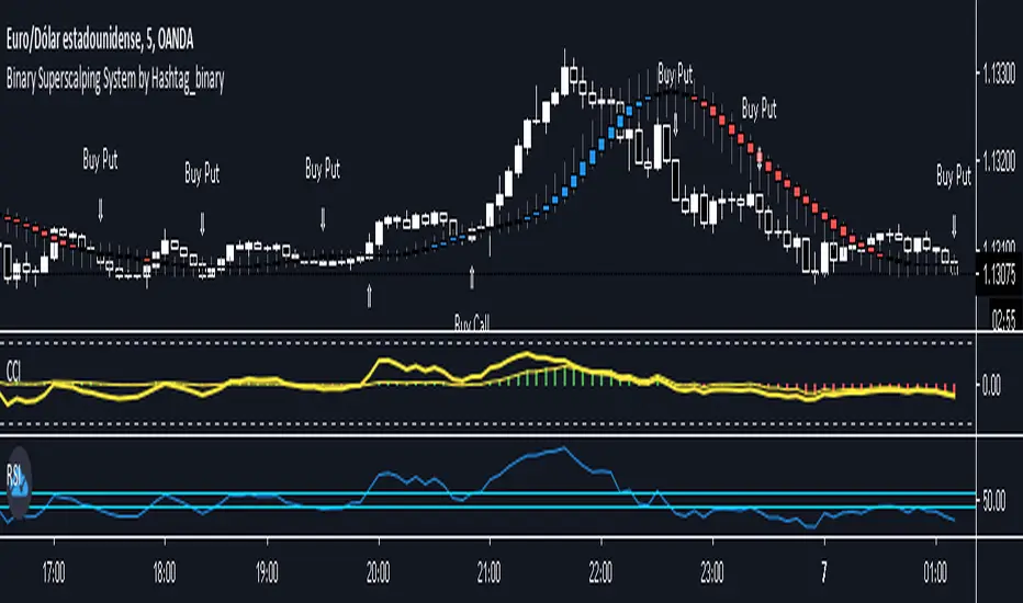
Binary Superscalping System by Hashtag_binaryBinary Superscalping Systyemis a trend momentum strategy designed for scalping and trading with binary options. This trading system is very accurate with the 80% profitable trades.
- Markets: Forex (EUR/USD, GBP/USD, AUD/USD, USD/CHF, USD/CAD, NZF/USD, USD/JPY,) Indicies (S&P500, Dow Jones, DAX, FTSE100) and Gold.
- Time Frame 5 min, 15min, 30min.
- Expiry Time (4-6 candles).
Buy Call or Buy:
- Trend CCI (170) crossed the zero line upwards (green bar >0);
- Entry CCI (34) crosses upward the zero line ;
- RSI (Relative Strength Index) indicator value is greater than 55 level;
- Heiken Ashi Smoothed indicator is color blue (optional).
Buy Put or Sell
- Trend CCI (170) crossed the zero line downwards (red bar <0);
- Entry CCI (34) crosses downward the zero line ;
- RSI indicator value is lower than 45 level;
- Heiken Ashi Smoothed indicator is color red (optiona).
Exit position for Scalping options:
- Entry CCI (34) crosses in opposite direction trend CCI (170),
- Profit Target:5 min time frame 7-10 pips, 15 min time frame (9-14 pips), 30 min time frame (15- 18 pips).
- Make Profit at fibopivot levels.
- Initial stop loss on the previous swing.
NimblrTACode written by Krishna Khanna on 04/11/2017 and includes the following components
1) CCI MTF
This indicator will draw the following
CCI-8 on 5 minutes
CCI-34 on 5 minutes
CCI-34 on 30 minutes interval on 5 minutes
2) Strength Candle Detection
This is put a * over any strength candle
3) EMA
This will plot EMA 5, EMA 21 and EMA 55
4) Panchang Time
Includes Pre-open and 4 timeslots
5) ORB Logic
ORBH and ORBL are plotted
6) Fibonacci Levels
Levels 0.618, 1 and 1.618 are plotted
7) Highest High and Lowest Low Strength Candles detected with CCI > 100 and CCI< -100 and indicated bye CCI_BO_B and CCI_BO_S

VB-MainLiteVB-MainLite – v1.0 Initial Release
Overview
VB-MainLite is a consolidated market-structure and execution framework designed to streamline decision-making into a single chart-level view. The script combines multi-timeframe trend, volatility, volume, and liquidity signals into one cohesive visual layer, reducing indicator clutter while preserving depth of information for active traders.
Core Architecture
Trend Backbone – EMA 200
Dedicated EMA 200 acts as the primary trend filter and higher-timeframe bias reference.
Serves as the “spine” of the system for contextualizing all secondary signals (swings, reversals, volume events, etc.).
Custom MA Suite (Envelope Ready)
Four configurable moving averages with flexible source, length, and smoothing.
Default configuration (preset idea: “8/89 Envelope”):
MA #1: EMA 8 on high
MA #2: EMA 8 on low
MA #3: EMA 89 on high
MA #4: EMA 89 on low
All four are disabled by default to keep the chart minimal. Users can toggle them on from the Custom MAs group for envelope or cloud-style configurations.
Nadaraya–Watson Smoother (Swing Framework)
Gaussian-kernel Nadaraya–Watson regression applied to price (hl2) to build a smooth synthetic curve.
Two layers of functionality:
Swing labels (▲ / ▼) at inflection points in the smoothed curve.
Optional curve line that visually tracks the turning structure over the last ~500 bars.
Designed to surface early swing potential before standard MAs react.
Hull Moving Average (Trend Overlay)
Optional Hull MA (HMA) for faster trend visualization.
Color-coded by slope (buy/sell bias).
Default: off to prevent overloading the chart; can be enabled under Hull MA settings.
Momentum, Exhaustion & Pattern Engine
CCI-Based Bar Coloring
CCI applied to close with configurable thresholds.
Overbought / oversold CCI zones map directly into candle coloring to visually highlight short-term momentum extremes.
RSI Top / Bottom Exhaustion Finder
RSI logic applied separately to high-driven (tops) and low-driven (bottoms) sequences.
Plots:
Top arrows where high-side RSI stretches into high-risk territory.
Bottom arrows where low-side RSI indicates exhaustion on the downside.
Useful as confluence around the Nadaraya swing turns and EMA 200 regime.
Engulfing + MA Trend Engine (“Fat Bull / Fat Bear”)
Detects bullish and bearish engulfing patterns, then combines them with MA trend cross logic.
Only when both pattern and MA regime align does the engine flag:
Fat Bull (Engulf + MA aligned long)
Fat Bear (Engulf + MA aligned short)
Candles are marked via conditional barcolor to highlight strong, structured shifts in control.
Fat Finger Detection (Wick Spikes / Stop Runs)
Identifies abnormal wick extensions relative to the prior bar’s body range with configurable tolerance.
Supports detection of potential liquidity grabs, stop runs, or “excess” that may precede reversals or mean-reversion behavior.
Volume & Liquidity Intelligence
Bull Snort (Aggressive Buy Spikes)
Flags events where:
Volume is significantly above the 50-period average, and
Price closes in the upper portion of the bar and above prior close.
Plots a labeled marker below the bar to indicate aggressive upside initiative by buyers.
Pocket Pivots (Accumulation Flags)
Compares current volume vs prior 10 sessions with a filter on prior “up” days.
Highlights pocket pivot days where current green candle volume outclasses recent down-day volumes, suggesting stealth accumulation.
Delta Volume Core (Directional Volume by Price)
Internal volume-by-price style engine over a user-defined lookback.
Splits volume into up-close and down-close buckets across dynamic price bins.
Feeds into S&R and ICT zone logic to quantify where buying vs selling pressure built up.
Structural Context: S&R and ICT Zones
S&R Power Channel
Computes local high/low band over a configurable lookback window.
Renders:
Upper and lower S&R channel lines.
Shaded support / resistance zones using boxes.
Adds Buy Power / Sell Power metrics based on the ratio of up vs down bars inside the window, displayed directly in the zone overlays.
Drops ◈ markers where price interacts dynamically with the top or bottom band, highlighting reaction points.
ICT-Style Premium / Discount & Macro Zones
Two tiered structures:
Local Premium / Discount zones over a shorter SR window.
Macro Premium / Discount zones over a longer macro window.
Each zone:
Uses underlying directional volume to annotate accumulation vs distribution bias.
Provides Delta Volume Bias shading in the mid-band region, visually encoding whether local power flows are net-buying or net-selling.
Enables traders to quickly see whether current trade location is in a local/macro discount or premium context while still respecting volume profile.
Positioning Intelligence: PCD (Stocks)
Position Cost Distribution (PCD) – Stocks Only
Available for stock symbols on intraday up to daily timeframe (≤ 1D).
Uses:
TOTAL_SHARES_OUTSTANDING fundamentals,
Daily OHLCV snapshot, and
A bucketed distribution engine
to approximate cost basis distribution across price.
Outputs:
Horizontal “PCD bars” to the right of current price, density-scaled by estimated share concentration.
Color-coding by profitability relative to current price (profitable vs unprofitable positions).
Labels for:
Current price
Average cost
Profit ratio (share % below current price)
90% cost range
70% cost range
Range overlap as a measure of clustering / concentration.
Multi-Timeframe Trend: Two-Pole Gaussian Dashboard
Two-Pole Gaussian Filter (Line + Cloud)
Smooths a user-selected source (default: close) using a two-pole Gaussian filter with tunable alpha.
Plots:
A thin Gaussian trend line, and
A thick Gaussian “cloud” line with transparency, colored by slope vs past (offsetG).
Functions as a responsive trend backbone that is more sensitive than EMA 200 but less noisy than raw price.
Multi-Timeframe Gaussian Dashboard
Evaluates Gaussian trend direction across up to six timeframes (e.g., 1H / 2H / 4H / Daily / Weekly).
Renders a compact bottom-right table:
Header: symbol + overall bias arrow (up / down) based on average trend alignment.
Row of colored cells per timeframe (green for uptrend, magenta for downtrend) with human-readable TF labels (e.g., “60M”, “4H”, “1D”).
Gives an immediate read on whether intraday, swing, and higher-timeframe flows are aligned or fragmented.
Default Configuration & Usage Guidance
Default state after adding the script:
Enabled by default:
EMA 200 trend backbone
Nadaraya–Watson swing labels and curve
CCI bar coloring
RSI top/bottom arrows
Fat Bull / Fat Bear engine
Bull Snort & Pocket Pivots
S&R Power Channel
ICT Local + Macro zones
Two-pole Gaussian line + cloud + dashboard
PCD engine for stocks (auto-active where data is available)
Disabled by default (opt-in):
Custom MA suite (4x MAs, preset as EMA 8/8/89/89)
Hull MA overlay
How traders can use VB-MainLite in practice:
Use EMA 200 + Gaussian dashboard to define top-down directional bias and avoid trading directly against multi-TF trend.
Use Nadaraya swing labels, RSI exhaustion arrows, and CCI bar colors to time entries within that higher-timeframe bias.
Use Fat Bull / Fat Bear events as structured confirmation that both pattern and MA regime have flipped in the same direction.
Use Bull Snort, Pocket Pivots, and S&R / ICT zones to align execution with liquidity, volume, and location (premium vs discount).
On stocks, use PCD as a positioning map to understand trapped supply, support zones near crowded cost basis, and where profit-taking is likely.

XAU Power Meter + HTF FVG SystemWhat is this?
XAU Power Meter + HTF FVG System is an execution-support tool for XAUUSD that combines:
Local trend & momentum on your entry timeframe (e.g. 5m)
Volatility regime (ATR)
Higher-timeframe FVG bias (e.g. 1H)
The goal is simple: filter out low-quality trades and size up only when the market actually moves.
Core Components
1. LTF Trend (MA Stack 20 / 50 / 200)
The indicator builds a “stacked trend” using three MAs:
Bullish trend → price > MA20 > MA50 > MA200
Bearish trend → price < MA20 < MA50 < MA200
Anything else → RANGE
This gives a clean directional bias for intraday execution.
2. CCI Impulse (“Power”)
The CCI block measures the strength of the current move via |CCI| and classifies it into 4 bands:
LOW – weak momentum, usually not worth it
MEDIUM – acceptable impulse
HIGH – strong impulse
EXTREME – very strong, potential blow-off / late entry zone
These bands are used both for signal quality (Grade) and for position size guidance.
3. ATR Volatility Regime
ATR(14) is compared against its own SMA(100) to classify volatility:
QUIET – ATR < K * ATR_slow
NORMAL
ACTIVE – ATR > K * ATR_slow
You don’t want to size up in a dead market. ATR regime is used inside the Grade calculation.
4. Grade System (A / B / C / X)
The indicator compresses Trend + CCI + ATR into a single Grade:
A – In trend, strong impulse (HIGH/EXTREME), active volatility → top setups
B – In trend, at least MEDIUM impulse, acceptable volatility → good setups
C – In trend, but weaker conditions → borderline, be selective
X – Out of trend or no momentum → avoid
Internally, execution signals require Grade ≥ B for two bars in a row, to avoid one-bar “fake” spikes.
5. HTF FVG Bias (e.g. 1H)
On a higher timeframe (default: 1H), the script runs a Fair Value Gap engine with:
EMA 50/200 trend filter
ATR-based body filter (minimum candle strength)
Wilder ADX filter (trend strength)
Deep retest requirement inside the FVG zone
Optional zone auto-expiry and delete-on-use
It returns:
BUY (bullish HTF FVG confirmed)
SELL (bearish HTF FVG confirmed)
NONE (no valid zone active)
You can control how strict this bias is used via a “Strict: require active HTF FVG for entry” checkbox:
Strict OFF (default) → HTF bias can block trades against a strong HTF signal, but allows trades when HTF is neutral.
Strict ON → LTF entries are allowed only when HTF has an active FVG in the same direction (very selective).
HTF events are shown on the chart as HTF BUY / HTF SELL markers.
Execution Signals (LTF LONG / SHORT)
On your entry timeframe (e.g. 5m), the script generates LONG / SHORT arrows when:
Trend is clearly bullish or bearish (MA stack aligned),
Grade ≥ B for two consecutive bars,
HTF bias conditions are satisfied (depending on the strict mode).
These arrows are not a full auto-strategy, but a high-quality execution cue:
“Trend OK + Momentum OK + Volatility OK + HTF not against you.”
Dashboard
A compact dashboard in the corner shows, in real time:
Trend – UP / DOWN / RANGE (20/50/200 stack)
Impulse (CCI) – LOW / MEDIUM / HIGH / EXTREME
Volatility (ATR) – QUIET / NORMAL / ACTIVE
Size Multiplier – suggested risk sizing factor based on impulse
Grade – A / B / C / X
HTF FVG – BUY / SELL / NONE
This lets you sanity-check the context before pressing the button, not after the loss.
Recommended Use
Instrument: XAUUSD
Timeframe: 5m (scalping / intraday), but can be tested on 15m/1H as well
HTF: 1H by default (can experiment with 4H)
Focus on:
Grade A/B only
Strict mode ON for more institutional, fewer but higher-quality trades
Size up only when both impulse and volatility are supportive
Disclaimer
This script is a decision-support tool, not financial advice and not a guarantee of profit.
Always forward-test, understand the logic, and use your own risk management.

TradeScope: MA Reversion • RVOL • Trendlines • GAPs • TableTradeScope is an all-in-one technical analysis suite that brings together price action, momentum, volume dynamics, and trend structure into one cohesive and fully customizable indicator.
An advanced, modular trading suite that combines moving averages, reversion signals, RSI/CCI momentum, relative volume, gap detection, trendline analysis, and dynamic tables — all within one powerful dashboard.
Perfect for swing traders, intraday traders, and analysts who want to read price strength, volume context, and market structure in real time.
⚙️ Core Components & Inputs
🧮 Moving Average Settings
Moving Average Type & Length:
Choose between SMA or EMA and set your preferred period for smoother or more reactive trend tracking.
Multi-MA Plotting:
Up to 8 customizable moving averages (each with independent type, color, and length).
Includes a “window filter” to show only the last X bars, reducing chart clutter.
MA Reversion Engine:
Detects when price has extended too far from its moving average.
Reversion Lookback: Number of bars analyzed to determine historical extremes.
Reversion Threshold: Sensitivity multiplier—lower = more frequent signals, higher = stricter triggers.
🔄 Trend Settings
Short-Term & Long-Term Trend Lookbacks:
Uses linear regression to detect the slope and direction of the short- and long-term trend.
Results are displayed in the live table with color-coded bias:
🟩 Bullish | 🟥 Bearish
📈 Momentum Indicators
RSI (Relative Strength Index):
Adjustable period; displays the current RSI value, overbought (>70) / oversold (<30) zones, and trending direction.
CCI (Commodity Channel Index):
Customizable length with color-coded bias:
🟩 Oversold (< -100), 🟥 Overbought (> 100).
Tooltip shows whether the CCI is trending up or down.
📊 Volume Analysis
Relative Volume (RVOL):
Estimates end-of-day projected volume using intraday progress and compares it against the 20-day average.
Displays whether today’s volume is expected to exceed yesterday’s, and highlights color by strength.
Volume Trend (Short & Long Lookbacks):
Visual cues for whether current volume is above or below short-term and long-term averages.
Estimated Full-Day Volume & Multiplier:
Converts raw volume into “X” multiples (e.g., 2.3X average) for quick interpretation.
🕳️ Gap Detection
Automatically identifies and plots bullish and bearish price gaps within a defined lookback period.
Gap Lookback: Defines how far back to search for gaps.
Gap Line Width / Visibility: Controls the thickness and display of gap lines on chart.
Displays the closest open gap in the live table, including its distance from current price (%).
🔍 ATR & Volatility
14-day ATR (% of price):
Automatically converts the Average True Range into a percent, providing quick volatility context:
🟩 Low (<3%) | 🟨 Moderate (3–5%) | 🟥 High (>5%)
💬 Candlestick Pattern Recognition
Auto-detects popular reversal and continuation patterns such as:
Bullish/Bearish Engulfing
Hammer / Hanging Man
Shooting Star / Inverted Hammer
Doji / Harami / Kicking / Marubozu / Morning Star
Each pattern is shown with contextual color coding in the table.
🧱 Pivot Points & Support/Resistance
Optional Pivot High / Pivot Low Labels
Adjustable left/right bar lengths for pivot detection
Theme-aware text and label color options
Automatically drawn diagonal trendlines for both support and resistance
Adjustable line style, color, and thickness
Detects and tracks touches for reliability
Includes breakout alerts (with optional volume confirmation)
🚨 Alerts
MA Cross Alerts:
Triggers when price crosses the fast or slow moving average within a tolerance band (default ±0.3%).
Diagonal Breakout Alerts:
Detects and alerts when price breaks diagonal trendlines.
Volume-Confirmed Alerts:
Filters breakouts where volume exceeds 1.5× the 20-bar average.
🧾 Live Market Table
A fully dynamic table displayed on-chart, customizable via input toggles:
Choose which rows to show (e.g., RSI, ATR, RVOL, Gaps, CCI, Trend, MA info, Diff, Low→Close%).
Choose table position (top-right, bottom-left, etc.) and text size.
Theme selection: Light or Dark
Conditional background colors for instant visual interpretation:
🟩 Bullish or Oversold
🟥 Bearish or Overbought
🟨 Neutral / Moderate
🎯 Practical Uses
✅ Identify confluence setups combining MA reversion, volume expansion, and RSI/CCI extremes.
✅ Track trend bias and gap proximity directly in your dashboard.
✅ Monitor relative volume behavior for intraday strength confirmation.
✅ Automate MA cross or breakout alerts to stay ahead of key price action.
🧠 Ideal For
Swing traders seeking confluence-based setups
Intraday traders monitoring multi-factor bias
Analysts looking for compact market health dashboards
💡 Summary
TradeScope is designed as a single-pane-of-glass market view — combining momentum, trend, volume, structure, and reversion into one clear visual system.
Fully customizable. Fully dynamic.
Use it to see what others miss — clarity, confluence, and confidence in every trade.

Markov Chain [3D] | FractalystWhat exactly is a Markov Chain?
This indicator uses a Markov Chain model to analyze, quantify, and visualize the transitions between market regimes (Bull, Bear, Neutral) on your chart. It dynamically detects these regimes in real-time, calculates transition probabilities, and displays them as animated 3D spheres and arrows, giving traders intuitive insight into current and future market conditions.
How does a Markov Chain work, and how should I read this spheres-and-arrows diagram?
Think of three weather modes: Sunny, Rainy, Cloudy.
Each sphere is one mode. The loop on a sphere means “stay the same next step” (e.g., Sunny again tomorrow).
The arrows leaving a sphere show where things usually go next if they change (e.g., Sunny moving to Cloudy).
Some paths matter more than others. A more prominent loop means the current mode tends to persist. A more prominent outgoing arrow means a change to that destination is the usual next step.
Direction isn’t symmetric: moving Sunny→Cloudy can behave differently than Cloudy→Sunny.
Now relabel the spheres to markets: Bull, Bear, Neutral.
Spheres: market regimes (uptrend, downtrend, range).
Self‑loop: tendency for the current regime to continue on the next bar.
Arrows: the most common next regime if a switch happens.
How to read: Start at the sphere that matches current bar state. If the loop stands out, expect continuation. If one outgoing path stands out, that switch is the typical next step. Opposite directions can differ (Bear→Neutral doesn’t have to match Neutral→Bear).
What states and transitions are shown?
The three market states visualized are:
Bullish (Bull): Upward or strong-market regime.
Bearish (Bear): Downward or weak-market regime.
Neutral: Sideways or range-bound regime.
Bidirectional animated arrows and probability labels show how likely the market is to move from one regime to another (e.g., Bull → Bear or Neutral → Bull).
How does the regime detection system work?
You can use either built-in price returns (based on adaptive Z-score normalization) or supply three custom indicators (such as volume, oscillators, etc.).
Values are statistically normalized (Z-scored) over a configurable lookback period.
The normalized outputs are classified into Bull, Bear, or Neutral zones.
If using three indicators, their regime signals are averaged and smoothed for robustness.
How are transition probabilities calculated?
On every confirmed bar, the algorithm tracks the sequence of detected market states, then builds a rolling window of transitions.
The code maintains a transition count matrix for all regime pairs (e.g., Bull → Bear).
Transition probabilities are extracted for each possible state change using Laplace smoothing for numerical stability, and frequently updated in real-time.
What is unique about the visualization?
3D animated spheres represent each regime and change visually when active.
Animated, bidirectional arrows reveal transition probabilities and allow you to see both dominant and less likely regime flows.
Particles (moving dots) animate along the arrows, enhancing the perception of regime flow direction and speed.
All elements dynamically update with each new price bar, providing a live market map in an intuitive, engaging format.
Can I use custom indicators for regime classification?
Yes! Enable the "Custom Indicators" switch and select any three chart series as inputs. These will be normalized and combined (each with equal weight), broadening the regime classification beyond just price-based movement.
What does the “Lookback Period” control?
Lookback Period (default: 100) sets how much historical data builds the probability matrix. Shorter periods adapt faster to regime changes but may be noisier. Longer periods are more stable but slower to adapt.
How is this different from a Hidden Markov Model (HMM)?
It sets the window for both regime detection and probability calculations. Lower values make the system more reactive, but potentially noisier. Higher values smooth estimates and make the system more robust.
How is this Markov Chain different from a Hidden Markov Model (HMM)?
Markov Chain (as here): All market regimes (Bull, Bear, Neutral) are directly observable on the chart. The transition matrix is built from actual detected regimes, keeping the model simple and interpretable.
Hidden Markov Model: The actual regimes are unobservable ("hidden") and must be inferred from market output or indicator "emissions" using statistical learning algorithms. HMMs are more complex, can capture more subtle structure, but are harder to visualize and require additional machine learning steps for training.
A standard Markov Chain models transitions between observable states using a simple transition matrix, while a Hidden Markov Model assumes the true states are hidden (latent) and must be inferred from observable “emissions” like price or volume data. In practical terms, a Markov Chain is transparent and easier to implement and interpret; an HMM is more expressive but requires statistical inference to estimate hidden states from data.
Markov Chain: states are observable; you directly count or estimate transition probabilities between visible states. This makes it simpler, faster, and easier to validate and tune.
HMM: states are hidden; you only observe emissions generated by those latent states. Learning involves machine learning/statistical algorithms (commonly Baum–Welch/EM for training and Viterbi for decoding) to infer both the transition dynamics and the most likely hidden state sequence from data.
How does the indicator avoid “repainting” or look-ahead bias?
All regime changes and matrix updates happen only on confirmed (closed) bars, so no future data is leaked, ensuring reliable real-time operation.
Are there practical tuning tips?
Tune the Lookback Period for your asset/timeframe: shorter for fast markets, longer for stability.
Use custom indicators if your asset has unique regime drivers.
Watch for rapid changes in transition probabilities as early warning of a possible regime shift.
Who is this indicator for?
Quants and quantitative researchers exploring probabilistic market modeling, especially those interested in regime-switching dynamics and Markov models.
Programmers and system developers who need a probabilistic regime filter for systematic and algorithmic backtesting:
The Markov Chain indicator is ideally suited for programmatic integration via its bias output (1 = Bull, 0 = Neutral, -1 = Bear).
Although the visualization is engaging, the core output is designed for automated, rules-based workflows—not for discretionary/manual trading decisions.
Developers can connect the indicator’s output directly to their Pine Script logic (using input.source()), allowing rapid and robust backtesting of regime-based strategies.
It acts as a plug-and-play regime filter: simply plug the bias output into your entry/exit logic, and you have a scientifically robust, probabilistically-derived signal for filtering, timing, position sizing, or risk regimes.
The MC's output is intentionally "trinary" (1/0/-1), focusing on clear regime states for unambiguous decision-making in code. If you require nuanced, multi-probability or soft-label state vectors, consider expanding the indicator or stacking it with a probability-weighted logic layer in your scripting.
Because it avoids subjectivity, this approach is optimal for systematic quants, algo developers building backtested, repeatable strategies based on probabilistic regime analysis.
What's the mathematical foundation behind this?
The mathematical foundation behind this Markov Chain indicator—and probabilistic regime detection in finance—draws from two principal models: the (standard) Markov Chain and the Hidden Markov Model (HMM).
How to use this indicator programmatically?
The Markov Chain indicator automatically exports a bias value (+1 for Bullish, -1 for Bearish, 0 for Neutral) as a plot visible in the Data Window. This allows you to integrate its regime signal into your own scripts and strategies for backtesting, automation, or live trading.
Step-by-Step Integration with Pine Script (input.source)
Add the Markov Chain indicator to your chart.
This must be done first, since your custom script will "pull" the bias signal from the indicator's plot.
In your strategy, create an input using input.source()
Example:
//@version=5
strategy("MC Bias Strategy Example")
mcBias = input.source(close, "MC Bias Source")
After saving, go to your script’s settings. For the “MC Bias Source” input, select the plot/output of the Markov Chain indicator (typically its bias plot).
Use the bias in your trading logic
Example (long only on Bull, flat otherwise):
if mcBias == 1
strategy.entry("Long", strategy.long)
else
strategy.close("Long")
For more advanced workflows, combine mcBias with additional filters or trailing stops.
How does this work behind-the-scenes?
TradingView’s input.source() lets you use any plot from another indicator as a real-time, “live” data feed in your own script (source).
The selected bias signal is available to your Pine code as a variable, enabling logical decisions based on regime (trend-following, mean-reversion, etc.).
This enables powerful strategy modularity : decouple regime detection from entry/exit logic, allowing fast experimentation without rewriting core signal code.
Integrating 45+ Indicators with Your Markov Chain — How & Why
The Enhanced Custom Indicators Export script exports a massive suite of over 45 technical indicators—ranging from classic momentum (RSI, MACD, Stochastic, etc.) to trend, volume, volatility, and oscillator tools—all pre-calculated, centered/scaled, and available as plots.
// Enhanced Custom Indicators Export - 45 Technical Indicators
// Comprehensive technical analysis suite for advanced market regime detection
//@version=6
indicator('Enhanced Custom Indicators Export | Fractalyst', shorttitle='Enhanced CI Export', overlay=false, scale=scale.right, max_labels_count=500, max_lines_count=500)
// |----- Input Parameters -----| //
momentum_group = "Momentum Indicators"
trend_group = "Trend Indicators"
volume_group = "Volume Indicators"
volatility_group = "Volatility Indicators"
oscillator_group = "Oscillator Indicators"
display_group = "Display Settings"
// Common lengths
length_14 = input.int(14, "Standard Length (14)", minval=1, maxval=100, group=momentum_group)
length_20 = input.int(20, "Medium Length (20)", minval=1, maxval=200, group=trend_group)
length_50 = input.int(50, "Long Length (50)", minval=1, maxval=200, group=trend_group)
// Display options
show_table = input.bool(true, "Show Values Table", group=display_group)
table_size = input.string("Small", "Table Size", options= , group=display_group)
// |----- MOMENTUM INDICATORS (15 indicators) -----| //
// 1. RSI (Relative Strength Index)
rsi_14 = ta.rsi(close, length_14)
rsi_centered = rsi_14 - 50
// 2. Stochastic Oscillator
stoch_k = ta.stoch(close, high, low, length_14)
stoch_d = ta.sma(stoch_k, 3)
stoch_centered = stoch_k - 50
// 3. Williams %R
williams_r = ta.stoch(close, high, low, length_14) - 100
// 4. MACD (Moving Average Convergence Divergence)
= ta.macd(close, 12, 26, 9)
// 5. Momentum (Rate of Change)
momentum = ta.mom(close, length_14)
momentum_pct = (momentum / close ) * 100
// 6. Rate of Change (ROC)
roc = ta.roc(close, length_14)
// 7. Commodity Channel Index (CCI)
cci = ta.cci(close, length_20)
// 8. Money Flow Index (MFI)
mfi = ta.mfi(close, length_14)
mfi_centered = mfi - 50
// 9. Awesome Oscillator (AO)
ao = ta.sma(hl2, 5) - ta.sma(hl2, 34)
// 10. Accelerator Oscillator (AC)
ac = ao - ta.sma(ao, 5)
// 11. Chande Momentum Oscillator (CMO)
cmo = ta.cmo(close, length_14)
// 12. Detrended Price Oscillator (DPO)
dpo = close - ta.sma(close, length_20)
// 13. Price Oscillator (PPO)
ppo = ta.sma(close, 12) - ta.sma(close, 26)
ppo_pct = (ppo / ta.sma(close, 26)) * 100
// 14. TRIX
trix_ema1 = ta.ema(close, length_14)
trix_ema2 = ta.ema(trix_ema1, length_14)
trix_ema3 = ta.ema(trix_ema2, length_14)
trix = ta.roc(trix_ema3, 1) * 10000
// 15. Klinger Oscillator
klinger = ta.ema(volume * (high + low + close) / 3, 34) - ta.ema(volume * (high + low + close) / 3, 55)
// 16. Fisher Transform
fisher_hl2 = 0.5 * (hl2 - ta.lowest(hl2, 10)) / (ta.highest(hl2, 10) - ta.lowest(hl2, 10)) - 0.25
fisher = 0.5 * math.log((1 + fisher_hl2) / (1 - fisher_hl2))
// 17. Stochastic RSI
stoch_rsi = ta.stoch(rsi_14, rsi_14, rsi_14, length_14)
stoch_rsi_centered = stoch_rsi - 50
// 18. Relative Vigor Index (RVI)
rvi_num = ta.swma(close - open)
rvi_den = ta.swma(high - low)
rvi = rvi_den != 0 ? rvi_num / rvi_den : 0
// 19. Balance of Power (BOP)
bop = (close - open) / (high - low)
// |----- TREND INDICATORS (10 indicators) -----| //
// 20. Simple Moving Average Momentum
sma_20 = ta.sma(close, length_20)
sma_momentum = ((close - sma_20) / sma_20) * 100
// 21. Exponential Moving Average Momentum
ema_20 = ta.ema(close, length_20)
ema_momentum = ((close - ema_20) / ema_20) * 100
// 22. Parabolic SAR
sar = ta.sar(0.02, 0.02, 0.2)
sar_trend = close > sar ? 1 : -1
// 23. Linear Regression Slope
lr_slope = ta.linreg(close, length_20, 0) - ta.linreg(close, length_20, 1)
// 24. Moving Average Convergence (MAC)
mac = ta.sma(close, 10) - ta.sma(close, 30)
// 25. Trend Intensity Index (TII)
tii_sum = 0.0
for i = 1 to length_20
tii_sum += close > close ? 1 : 0
tii = (tii_sum / length_20) * 100
// 26. Ichimoku Cloud Components
ichimoku_tenkan = (ta.highest(high, 9) + ta.lowest(low, 9)) / 2
ichimoku_kijun = (ta.highest(high, 26) + ta.lowest(low, 26)) / 2
ichimoku_signal = ichimoku_tenkan > ichimoku_kijun ? 1 : -1
// 27. MESA Adaptive Moving Average (MAMA)
mama_alpha = 2.0 / (length_20 + 1)
mama = ta.ema(close, length_20)
mama_momentum = ((close - mama) / mama) * 100
// 28. Zero Lag Exponential Moving Average (ZLEMA)
zlema_lag = math.round((length_20 - 1) / 2)
zlema_data = close + (close - close )
zlema = ta.ema(zlema_data, length_20)
zlema_momentum = ((close - zlema) / zlema) * 100
// |----- VOLUME INDICATORS (6 indicators) -----| //
// 29. On-Balance Volume (OBV)
obv = ta.obv
// 30. Volume Rate of Change (VROC)
vroc = ta.roc(volume, length_14)
// 31. Price Volume Trend (PVT)
pvt = ta.pvt
// 32. Negative Volume Index (NVI)
nvi = 0.0
nvi := volume < volume ? nvi + ((close - close ) / close ) * nvi : nvi
// 33. Positive Volume Index (PVI)
pvi = 0.0
pvi := volume > volume ? pvi + ((close - close ) / close ) * pvi : pvi
// 34. Volume Oscillator
vol_osc = ta.sma(volume, 5) - ta.sma(volume, 10)
// 35. Ease of Movement (EOM)
eom_distance = high - low
eom_box_height = volume / 1000000
eom = eom_box_height != 0 ? eom_distance / eom_box_height : 0
eom_sma = ta.sma(eom, length_14)
// 36. Force Index
force_index = volume * (close - close )
force_index_sma = ta.sma(force_index, length_14)
// |----- VOLATILITY INDICATORS (10 indicators) -----| //
// 37. Average True Range (ATR)
atr = ta.atr(length_14)
atr_pct = (atr / close) * 100
// 38. Bollinger Bands Position
bb_basis = ta.sma(close, length_20)
bb_dev = 2.0 * ta.stdev(close, length_20)
bb_upper = bb_basis + bb_dev
bb_lower = bb_basis - bb_dev
bb_position = bb_dev != 0 ? (close - bb_basis) / bb_dev : 0
bb_width = bb_dev != 0 ? (bb_upper - bb_lower) / bb_basis * 100 : 0
// 39. Keltner Channels Position
kc_basis = ta.ema(close, length_20)
kc_range = ta.ema(ta.tr, length_20)
kc_upper = kc_basis + (2.0 * kc_range)
kc_lower = kc_basis - (2.0 * kc_range)
kc_position = kc_range != 0 ? (close - kc_basis) / kc_range : 0
// 40. Donchian Channels Position
dc_upper = ta.highest(high, length_20)
dc_lower = ta.lowest(low, length_20)
dc_basis = (dc_upper + dc_lower) / 2
dc_position = (dc_upper - dc_lower) != 0 ? (close - dc_basis) / (dc_upper - dc_lower) : 0
// 41. Standard Deviation
std_dev = ta.stdev(close, length_20)
std_dev_pct = (std_dev / close) * 100
// 42. Relative Volatility Index (RVI)
rvi_up = ta.stdev(close > close ? close : 0, length_14)
rvi_down = ta.stdev(close < close ? close : 0, length_14)
rvi_total = rvi_up + rvi_down
rvi_volatility = rvi_total != 0 ? (rvi_up / rvi_total) * 100 : 50
// 43. Historical Volatility
hv_returns = math.log(close / close )
hv = ta.stdev(hv_returns, length_20) * math.sqrt(252) * 100
// 44. Garman-Klass Volatility
gk_vol = math.log(high/low) * math.log(high/low) - (2*math.log(2)-1) * math.log(close/open) * math.log(close/open)
gk_volatility = math.sqrt(ta.sma(gk_vol, length_20)) * 100
// 45. Parkinson Volatility
park_vol = math.log(high/low) * math.log(high/low)
parkinson = math.sqrt(ta.sma(park_vol, length_20) / (4 * math.log(2))) * 100
// 46. Rogers-Satchell Volatility
rs_vol = math.log(high/close) * math.log(high/open) + math.log(low/close) * math.log(low/open)
rogers_satchell = math.sqrt(ta.sma(rs_vol, length_20)) * 100
// |----- OSCILLATOR INDICATORS (5 indicators) -----| //
// 47. Elder Ray Index
elder_bull = high - ta.ema(close, 13)
elder_bear = low - ta.ema(close, 13)
elder_power = elder_bull + elder_bear
// 48. Schaff Trend Cycle (STC)
stc_macd = ta.ema(close, 23) - ta.ema(close, 50)
stc_k = ta.stoch(stc_macd, stc_macd, stc_macd, 10)
stc_d = ta.ema(stc_k, 3)
stc = ta.stoch(stc_d, stc_d, stc_d, 10)
// 49. Coppock Curve
coppock_roc1 = ta.roc(close, 14)
coppock_roc2 = ta.roc(close, 11)
coppock = ta.wma(coppock_roc1 + coppock_roc2, 10)
// 50. Know Sure Thing (KST)
kst_roc1 = ta.roc(close, 10)
kst_roc2 = ta.roc(close, 15)
kst_roc3 = ta.roc(close, 20)
kst_roc4 = ta.roc(close, 30)
kst = ta.sma(kst_roc1, 10) + 2*ta.sma(kst_roc2, 10) + 3*ta.sma(kst_roc3, 10) + 4*ta.sma(kst_roc4, 15)
// 51. Percentage Price Oscillator (PPO)
ppo_line = ((ta.ema(close, 12) - ta.ema(close, 26)) / ta.ema(close, 26)) * 100
ppo_signal = ta.ema(ppo_line, 9)
ppo_histogram = ppo_line - ppo_signal
// |----- PLOT MAIN INDICATORS -----| //
// Plot key momentum indicators
plot(rsi_centered, title="01_RSI_Centered", color=color.purple, linewidth=1)
plot(stoch_centered, title="02_Stoch_Centered", color=color.blue, linewidth=1)
plot(williams_r, title="03_Williams_R", color=color.red, linewidth=1)
plot(macd_histogram, title="04_MACD_Histogram", color=color.orange, linewidth=1)
plot(cci, title="05_CCI", color=color.green, linewidth=1)
// Plot trend indicators
plot(sma_momentum, title="06_SMA_Momentum", color=color.navy, linewidth=1)
plot(ema_momentum, title="07_EMA_Momentum", color=color.maroon, linewidth=1)
plot(sar_trend, title="08_SAR_Trend", color=color.teal, linewidth=1)
plot(lr_slope, title="09_LR_Slope", color=color.lime, linewidth=1)
plot(mac, title="10_MAC", color=color.fuchsia, linewidth=1)
// Plot volatility indicators
plot(atr_pct, title="11_ATR_Pct", color=color.yellow, linewidth=1)
plot(bb_position, title="12_BB_Position", color=color.aqua, linewidth=1)
plot(kc_position, title="13_KC_Position", color=color.olive, linewidth=1)
plot(std_dev_pct, title="14_StdDev_Pct", color=color.silver, linewidth=1)
plot(bb_width, title="15_BB_Width", color=color.gray, linewidth=1)
// Plot volume indicators
plot(vroc, title="16_VROC", color=color.blue, linewidth=1)
plot(eom_sma, title="17_EOM", color=color.red, linewidth=1)
plot(vol_osc, title="18_Vol_Osc", color=color.green, linewidth=1)
plot(force_index_sma, title="19_Force_Index", color=color.orange, linewidth=1)
plot(obv, title="20_OBV", color=color.purple, linewidth=1)
// Plot additional oscillators
plot(ao, title="21_Awesome_Osc", color=color.navy, linewidth=1)
plot(cmo, title="22_CMO", color=color.maroon, linewidth=1)
plot(dpo, title="23_DPO", color=color.teal, linewidth=1)
plot(trix, title="24_TRIX", color=color.lime, linewidth=1)
plot(fisher, title="25_Fisher", color=color.fuchsia, linewidth=1)
// Plot more momentum indicators
plot(mfi_centered, title="26_MFI_Centered", color=color.yellow, linewidth=1)
plot(ac, title="27_AC", color=color.aqua, linewidth=1)
plot(ppo_pct, title="28_PPO_Pct", color=color.olive, linewidth=1)
plot(stoch_rsi_centered, title="29_StochRSI_Centered", color=color.silver, linewidth=1)
plot(klinger, title="30_Klinger", color=color.gray, linewidth=1)
// Plot trend continuation
plot(tii, title="31_TII", color=color.blue, linewidth=1)
plot(ichimoku_signal, title="32_Ichimoku_Signal", color=color.red, linewidth=1)
plot(mama_momentum, title="33_MAMA_Momentum", color=color.green, linewidth=1)
plot(zlema_momentum, title="34_ZLEMA_Momentum", color=color.orange, linewidth=1)
plot(bop, title="35_BOP", color=color.purple, linewidth=1)
// Plot volume continuation
plot(nvi, title="36_NVI", color=color.navy, linewidth=1)
plot(pvi, title="37_PVI", color=color.maroon, linewidth=1)
plot(momentum_pct, title="38_Momentum_Pct", color=color.teal, linewidth=1)
plot(roc, title="39_ROC", color=color.lime, linewidth=1)
plot(rvi, title="40_RVI", color=color.fuchsia, linewidth=1)
// Plot volatility continuation
plot(dc_position, title="41_DC_Position", color=color.yellow, linewidth=1)
plot(rvi_volatility, title="42_RVI_Volatility", color=color.aqua, linewidth=1)
plot(hv, title="43_Historical_Vol", color=color.olive, linewidth=1)
plot(gk_volatility, title="44_GK_Volatility", color=color.silver, linewidth=1)
plot(parkinson, title="45_Parkinson_Vol", color=color.gray, linewidth=1)
// Plot final oscillators
plot(rogers_satchell, title="46_RS_Volatility", color=color.blue, linewidth=1)
plot(elder_power, title="47_Elder_Power", color=color.red, linewidth=1)
plot(stc, title="48_STC", color=color.green, linewidth=1)
plot(coppock, title="49_Coppock", color=color.orange, linewidth=1)
plot(kst, title="50_KST", color=color.purple, linewidth=1)
// Plot final indicators
plot(ppo_histogram, title="51_PPO_Histogram", color=color.navy, linewidth=1)
plot(pvt, title="52_PVT", color=color.maroon, linewidth=1)
// |----- Reference Lines -----| //
hline(0, "Zero Line", color=color.gray, linestyle=hline.style_dashed, linewidth=1)
hline(50, "Midline", color=color.gray, linestyle=hline.style_dotted, linewidth=1)
hline(-50, "Lower Midline", color=color.gray, linestyle=hline.style_dotted, linewidth=1)
hline(25, "Upper Threshold", color=color.gray, linestyle=hline.style_dotted, linewidth=1)
hline(-25, "Lower Threshold", color=color.gray, linestyle=hline.style_dotted, linewidth=1)
// |----- Enhanced Information Table -----| //
if show_table and barstate.islast
table_position = position.top_right
table_text_size = table_size == "Tiny" ? size.tiny : table_size == "Small" ? size.small : size.normal
var table info_table = table.new(table_position, 3, 18, bgcolor=color.new(color.white, 85), border_width=1, border_color=color.gray)
// Headers
table.cell(info_table, 0, 0, 'Category', text_color=color.black, text_size=table_text_size, bgcolor=color.new(color.blue, 70))
table.cell(info_table, 1, 0, 'Indicator', text_color=color.black, text_size=table_text_size, bgcolor=color.new(color.blue, 70))
table.cell(info_table, 2, 0, 'Value', text_color=color.black, text_size=table_text_size, bgcolor=color.new(color.blue, 70))
// Key Momentum Indicators
table.cell(info_table, 0, 1, 'MOMENTUM', text_color=color.purple, text_size=table_text_size, bgcolor=color.new(color.purple, 90))
table.cell(info_table, 1, 1, 'RSI Centered', text_color=color.purple, text_size=table_text_size)
table.cell(info_table, 2, 1, str.tostring(rsi_centered, '0.00'), text_color=color.purple, text_size=table_text_size)
table.cell(info_table, 0, 2, '', text_color=color.blue, text_size=table_text_size)
table.cell(info_table, 1, 2, 'Stoch Centered', text_color=color.blue, text_size=table_text_size)
table.cell(info_table, 2, 2, str.tostring(stoch_centered, '0.00'), text_color=color.blue, text_size=table_text_size)
table.cell(info_table, 0, 3, '', text_color=color.red, text_size=table_text_size)
table.cell(info_table, 1, 3, 'Williams %R', text_color=color.red, text_size=table_text_size)
table.cell(info_table, 2, 3, str.tostring(williams_r, '0.00'), text_color=color.red, text_size=table_text_size)
table.cell(info_table, 0, 4, '', text_color=color.orange, text_size=table_text_size)
table.cell(info_table, 1, 4, 'MACD Histogram', text_color=color.orange, text_size=table_text_size)
table.cell(info_table, 2, 4, str.tostring(macd_histogram, '0.000'), text_color=color.orange, text_size=table_text_size)
table.cell(info_table, 0, 5, '', text_color=color.green, text_size=table_text_size)
table.cell(info_table, 1, 5, 'CCI', text_color=color.green, text_size=table_text_size)
table.cell(info_table, 2, 5, str.tostring(cci, '0.00'), text_color=color.green, text_size=table_text_size)
// Key Trend Indicators
table.cell(info_table, 0, 6, 'TREND', text_color=color.navy, text_size=table_text_size, bgcolor=color.new(color.navy, 90))
table.cell(info_table, 1, 6, 'SMA Momentum %', text_color=color.navy, text_size=table_text_size)
table.cell(info_table, 2, 6, str.tostring(sma_momentum, '0.00'), text_color=color.navy, text_size=table_text_size)
table.cell(info_table, 0, 7, '', text_color=color.maroon, text_size=table_text_size)
table.cell(info_table, 1, 7, 'EMA Momentum %', text_color=color.maroon, text_size=table_text_size)
table.cell(info_table, 2, 7, str.tostring(ema_momentum, '0.00'), text_color=color.maroon, text_size=table_text_size)
table.cell(info_table, 0, 8, '', text_color=color.teal, text_size=table_text_size)
table.cell(info_table, 1, 8, 'SAR Trend', text_color=color.teal, text_size=table_text_size)
table.cell(info_table, 2, 8, str.tostring(sar_trend, '0'), text_color=color.teal, text_size=table_text_size)
table.cell(info_table, 0, 9, '', text_color=color.lime, text_size=table_text_size)
table.cell(info_table, 1, 9, 'Linear Regression', text_color=color.lime, text_size=table_text_size)
table.cell(info_table, 2, 9, str.tostring(lr_slope, '0.000'), text_color=color.lime, text_size=table_text_size)
// Key Volatility Indicators
table.cell(info_table, 0, 10, 'VOLATILITY', text_color=color.yellow, text_size=table_text_size, bgcolor=color.new(color.yellow, 90))
table.cell(info_table, 1, 10, 'ATR %', text_color=color.yellow, text_size=table_text_size)
table.cell(info_table, 2, 10, str.tostring(atr_pct, '0.00'), text_color=color.yellow, text_size=table_text_size)
table.cell(info_table, 0, 11, '', text_color=color.aqua, text_size=table_text_size)
table.cell(info_table, 1, 11, 'BB Position', text_color=color.aqua, text_size=table_text_size)
table.cell(info_table, 2, 11, str.tostring(bb_position, '0.00'), text_color=color.aqua, text_size=table_text_size)
table.cell(info_table, 0, 12, '', text_color=color.olive, text_size=table_text_size)
table.cell(info_table, 1, 12, 'KC Position', text_color=color.olive, text_size=table_text_size)
table.cell(info_table, 2, 12, str.tostring(kc_position, '0.00'), text_color=color.olive, text_size=table_text_size)
// Key Volume Indicators
table.cell(info_table, 0, 13, 'VOLUME', text_color=color.blue, text_size=table_text_size, bgcolor=color.new(color.blue, 90))
table.cell(info_table, 1, 13, 'Volume ROC', text_color=color.blue, text_size=table_text_size)
table.cell(info_table, 2, 13, str.tostring(vroc, '0.00'), text_color=color.blue, text_size=table_text_size)
table.cell(info_table, 0, 14, '', text_color=color.red, text_size=table_text_size)
table.cell(info_table, 1, 14, 'EOM', text_color=color.red, text_size=table_text_size)
table.cell(info_table, 2, 14, str.tostring(eom_sma, '0.000'), text_color=color.red, text_size=table_text_size)
// Key Oscillators
table.cell(info_table, 0, 15, 'OSCILLATORS', text_color=color.purple, text_size=table_text_size, bgcolor=color.new(color.purple, 90))
table.cell(info_table, 1, 15, 'Awesome Osc', text_color=color.blue, text_size=table_text_size)
table.cell(info_table, 2, 15, str.tostring(ao, '0.000'), text_color=color.blue, text_size=table_text_size)
table.cell(info_table, 0, 16, '', text_color=color.red, text_size=table_text_size)
table.cell(info_table, 1, 16, 'Fisher Transform', text_color=color.red, text_size=table_text_size)
table.cell(info_table, 2, 16, str.tostring(fisher, '0.000'), text_color=color.red, text_size=table_text_size)
// Summary Statistics
table.cell(info_table, 0, 17, 'SUMMARY', text_color=color.black, text_size=table_text_size, bgcolor=color.new(color.gray, 70))
table.cell(info_table, 1, 17, 'Total Indicators: 52', text_color=color.black, text_size=table_text_size)
regime_color = rsi_centered > 10 ? color.green : rsi_centered < -10 ? color.red : color.gray
regime_text = rsi_centered > 10 ? "BULLISH" : rsi_centered < -10 ? "BEARISH" : "NEUTRAL"
table.cell(info_table, 2, 17, regime_text, text_color=regime_color, text_size=table_text_size)
This makes it the perfect “indicator backbone” for quantitative and systematic traders who want to prototype, combine, and test new regime detection models—especially in combination with the Markov Chain indicator.
How to use this script with the Markov Chain for research and backtesting:
Add the Enhanced Indicator Export to your chart.
Every calculated indicator is available as an individual data stream.
Connect the indicator(s) you want as custom input(s) to the Markov Chain’s “Custom Indicators” option.
In the Markov Chain indicator’s settings, turn ON the custom indicator mode.
For each of the three custom indicator inputs, select the exported plot from the Enhanced Export script—the menu lists all 45+ signals by name.
This creates a powerful, modular regime-detection engine where you can mix-and-match momentum, trend, volume, or custom combinations for advanced filtering.
Backtest regime logic directly.
Once you’ve connected your chosen indicators, the Markov Chain script performs regime detection (Bull/Neutral/Bear) based on your selected features—not just price returns.
The regime detection is robust, automatically normalized (using Z-score), and outputs bias (1, -1, 0) for plug-and-play integration.
Export the regime bias for programmatic use.
As described above, use input.source() in your Pine Script strategy or system and link the bias output.
You can now filter signals, control trade direction/size, or design pairs-trading that respect true, indicator-driven market regimes.
With this framework, you’re not limited to static or simplistic regime filters. You can rigorously define, test, and refine what “market regime” means for your strategies—using the technical features that matter most to you.
Optimize your signal generation by backtesting across a universe of meaningful indicator blends.
Enhance risk management with objective, real-time regime boundaries.
Accelerate your research: iterate quickly, swap indicator components, and see results with minimal code changes.
Automate multi-asset or pairs-trading by integrating regime context directly into strategy logic.
Add both scripts to your chart, connect your preferred features, and start investigating your best regime-based trades—entirely within the TradingView ecosystem.
References & Further Reading
Ang, A., & Bekaert, G. (2002). “Regime Switches in Interest Rates.” Journal of Business & Economic Statistics, 20(2), 163–182.
Hamilton, J. D. (1989). “A New Approach to the Economic Analysis of Nonstationary Time Series and the Business Cycle.” Econometrica, 57(2), 357–384.
Markov, A. A. (1906). "Extension of the Limit Theorems of Probability Theory to a Sum of Variables Connected in a Chain." The Notes of the Imperial Academy of Sciences of St. Petersburg.
Guidolin, M., & Timmermann, A. (2007). “Asset Allocation under Multivariate Regime Switching.” Journal of Economic Dynamics and Control, 31(11), 3503–3544.
Murphy, J. J. (1999). Technical Analysis of the Financial Markets. New York Institute of Finance.
Brock, W., Lakonishok, J., & LeBaron, B. (1992). “Simple Technical Trading Rules and the Stochastic Properties of Stock Returns.” Journal of Finance, 47(5), 1731–1764.
Zucchini, W., MacDonald, I. L., & Langrock, R. (2017). Hidden Markov Models for Time Series: An Introduction Using R (2nd ed.). Chapman and Hall/CRC.
On Quantitative Finance and Markov Models:
Lo, A. W., & Hasanhodzic, J. (2009). The Heretics of Finance: Conversations with Leading Practitioners of Technical Analysis. Bloomberg Press.
Patterson, S. (2016). The Man Who Solved the Market: How Jim Simons Launched the Quant Revolution. Penguin Press.
TradingView Pine Script Documentation: www.tradingview.com
TradingView Blog: “Use an Input From Another Indicator With Your Strategy” www.tradingview.com
GeeksforGeeks: “What is the Difference Between Markov Chains and Hidden Markov Models?” www.geeksforgeeks.org
What makes this indicator original and unique?
- On‑chart, real‑time Markov. The chain is drawn directly on your chart. You see the current regime, its tendency to stay (self‑loop), and the usual next step (arrows) as bars confirm.
- Source‑agnostic by design. The engine runs on any series you select via input.source() — price, your own oscillator, a composite score, anything you compute in the script.
- Automatic normalization + regime mapping. Different inputs live on different scales. The script standardizes your chosen source and maps it into clear regimes (e.g., Bull / Bear / Neutral) without you micromanaging thresholds each time.
- Rolling, bar‑by‑bar learning. Transition tendencies are computed from a rolling window of confirmed bars. What you see is exactly what the market did in that window.
- Fast experimentation. Switch the source, adjust the window, and the Markov view updates instantly. It’s a rapid way to test ideas and feel regime persistence/switch behavior.
Integrate your own signals (using input.source())
- In settings, choose the Source . This is powered by input.source() .
- Feed it price, an indicator you compute inside the script, or a custom composite series.
- The script will automatically normalize that series and process it through the Markov engine, mapping it to regimes and updating the on‑chart spheres/arrows in real time.
Credits:
Deep gratitude to @RicardoSantos for both the foundational Markov chain processing engine and inspiring open-source contributions, which made advanced probabilistic market modeling accessible to the TradingView community.
Special thanks to @Alien_Algorithms for the innovative and visually stunning 3D sphere logic that powers the indicator’s animated, regime-based visualization.
Disclaimer
This tool summarizes recent behavior. It is not financial advice and not a guarantee of future results.

Momentum, Trend and Volatility indicator by [Th16rry]Momentum, Trend and Volatility indicator by
Description:
Momentum, Trend and Volatility indicator by is an advanced TradingView indicator designed to clearly identify market bias, volatility, and momentum directly on your charts. It integrates multiple analytical techniques, combining adaptive moving averages, volatility bands, and momentum signals into a unified visual framework.
Key Components:
Adaptive Moving Average (Nadaraya–Watson): A sophisticated, non-repainting adaptive moving average colored dynamically to instantly show bullish or bearish trends. This component highlights the prevailing market bias.
Trend Channel: Built around a central Keltner Channel with a customizable multiplier, this channel captures immediate price trends. When price remains within this channel, it indicates sustained market direction.
Volatility Channel: Represented by broader bands using a higher ATR multiplier. Price movements crossing outside these channels suggest significant volatility spikes, often signaling potential market reversals or strong breakout moves.
Range Channel: A medium ATR multiplier channel designed to pinpoint potential consolidation or ranging conditions. Useful for identifying short-term trading ranges or preparation phases before major moves.
CCI Momentum Signals: Includes optional Commodity Channel Index (CCI) signals to identify momentum shifts. Arrows appear when CCI crosses predefined thresholds, signaling potential overbought or oversold conditions.
How to Use:
Trend Following: Enter trades aligned with the adaptive moving average color. A teal line indicates bullish conditions, while a red line suggests bearish sentiment. Use Trend Channel
to spot Breakouts and pull-backs.
Volatility Breakouts: Pay attention to arrows marking price breaches beyond the Volatility Channel. Upward (red) and downward (green) arrows highlight significant breakout or reversal opportunities.
Range Trading: Utilize the Range Channel to trade sideways markets. Price reactions near these boundaries can offer quick reversal trade setups or scalping opportunities. Or simply avoid any trading during these low volatility phases.
Momentum Entries: Enable CCI signals to catch momentum-based trades. Green circles indicate bullish momentum turning points; red circles indicate bearish momentum shifts.
Customization:
Momentum, Trend and Volatility indicator by provides full customization to fit individual trading styles:
Adjust ATR multipliers to control channel widths.
Configure Nadaraya–Watson parameters for sensitivity.
Enable or disable visual elements such as channel backgrounds or CCI signals to maintain chart clarity.
This indicator serves as a comprehensive trading tool for traders looking to enhance their strategy through a clear understanding of market dynamics, including trend strength, volatility bursts, and momentum shifts.
Disclaimer:
Trading involves significant risk of loss and is not suitable for every investor. Always use proper risk management strategies. This Indicator is provided for educational purposes only and does not constitute financial advice or recommendations to trade specific assets. Users should conduct their own research and consult a licensed financial advisor before making trading decisions.
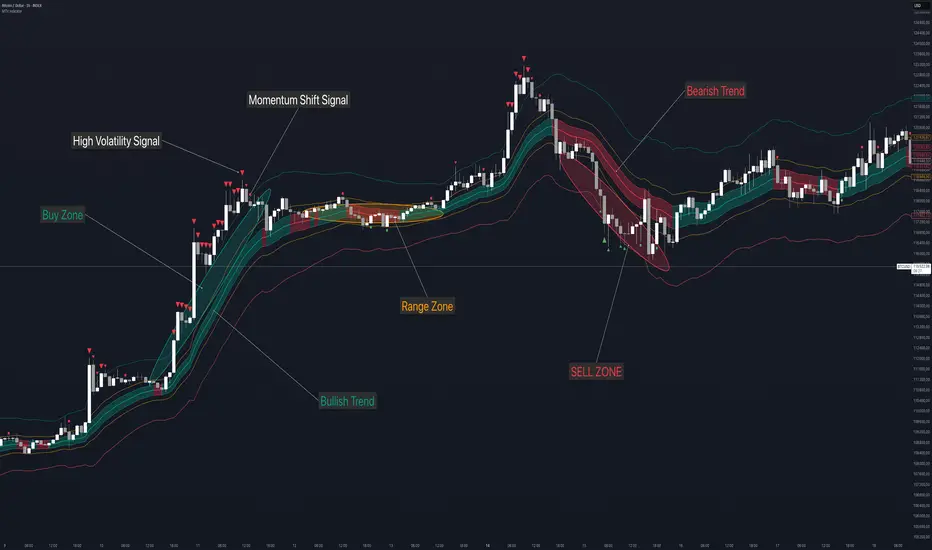
Gorgo's Hybrid Oscillator STrategy**Indicator Name:** Gorgo's Hybrid Oscillator STrategy (G.H.O.S.T.)
**Purpose:**
The Gorgo's Hybrid Oscillator STrategy (G.H.O.S.T.) is a multi-component technical analysis tool designed to identify overbought and oversold market conditions, assess trend strength, and signal potential buy and sell opportunities. By combining elements from RSI, Ultimate Oscillator, Stochastic CCI, and ADX, this custom indicator provides a comprehensive view of momentum, trend intensity, and volume context to enhance decision-making.
---
**Components and Logic:**
1. **RSI (Relative Strength Index):**
* Calculated using a customizable period (default: 14) and based on the hlc3 price source.
* Measures recent price changes to evaluate overbought/oversold conditions.
* Incorporated in the final oscillator average.
2. **Ultimate Oscillator:**
* Combines three timeframes (7, 14, 28 by default) to smooth out price movements.
* Uses true range and buying pressure for multi-frame momentum analysis.
* Averaged together with RSI to create the main oscillator signal.
3. **Stochastic CCI:**
* Applies a stochastic process to the Commodity Channel Index (CCI).
* Smooths the %K and %D lines (default: 3 each) to detect subtle reversals.
* Generates oversold (<35) and overbought (>69) signals, plotted as yellow circles.
4. **ADX + DI (Average Directional Index):**
* Determines trend strength using ADX and directional movement indicators (DI).
* ADX threshold is set at 24 by default to filter weak trends.
* Colored histogram columns:
* Green: Strong bullish trend.
* Red: Strong bearish trend.
* Gray: Weak/no trend.
5. **Volume Analysis:**
* Calculates a 9-period SMA of volume.
* Detects significant volume spikes (2.7× the average by default) to validate breakouts or fakeouts.
6. **Oscillator Output ("osc") and Levels:**
* The main plotted oscillator line is the average of the RSI and Ultimate Oscillator.
* Important horizontal lines:
* Overbought (69.0)
* Oversold (35.0)
* Midline (52.0): Neutral reference point.
* ADX threshold line (24.0)
---
**Signals:**
1. **Buy Signal Conditions:**
* Close is less than or equal to open (candle is red).
* Oscillator is decreasing and below oversold level.
* Stochastic CCI is below midline.
* Volume is above average, or excessive volume with oscillator falling below 40.
* ADX confirms trend presence (either above 15 or meeting threshold).
2. **Sell Signal Conditions:**
* ADX increasing and confirming trend.
* Oscillator is increasing and above overbought level.
* Stochastic CCI is above midline.
* Volume is above average, or very high with oscillator above 60.
3. **Visual Feedback:**
* Yellow dots highlight oversold/overbought Stochastic CCI.
* Oscillator line in cyan.
* Background colors:
* Light red for buy signals.
* White for sell signals.
4. **Alerts:**
* Built-in `alertcondition()` calls allow automated alerts for buy and sell events.
---
**Usage Guide:**
* **Best Use Cases:** Trend-following and reversal strategies on any timeframe.
* **Avoid Using Alone:** Use G.H.O.S.T. in conjunction with price action, support/resistance, and other confluence tools.
* **Customization:** All thresholds, periods, and volumes are user-editable from the settings panel.
---
**Interpretation Summary:**
G.H.O.S.T. excels at filtering out noise by combining different oscillators and volume signals to offer contextually valid entries and exits. A bullish (buy) signal typically suggests a market under pressure but potentially bottoming out, while a bearish (sell) signal highlights likely exhaustion after a strong upward push.
This hybrid approach makes the G.H.O.S.T. a reliable ally in volatile or choppy conditions where single-indicator strategies might fail.

AP IFTCCIv2/IFTStoch/IFTRSI Multi-TimeframeMulti-Timeframe IFT-CCI/Stoch/RSI Composite
This enhanced indicator combines three powerful oscillators—Inverse Fisher Transform (IFT) versions of the Commodity Channel Index (CCI), Stochastic, and Relative Strength Index (RSI)—into a unified multi-timeframe analysis tool. Originally developed by John Ehlers (pioneer of cyclical analysis and signal processing in trading systems) and adapted by KIVANC (@fr3762), this version adds dual-timeframe capability to compare indicator values across different chart resolutions.
Key Features:
Triple Oscillator Composite
IFT-CCI: Smoothed CCI values transformed via Ehlers' Inverse Fisher Transform (blue-gold)
IFT-Stochastic: Classic stochastic oscillator processed through IFT (blue)
IFT-RSI: RSI oscillator converted to IFT format (magenta)
Composite Average Line: Combined average of all three indicators (green)
Multi-Timeframe Analysis
Compare primary and secondary timeframes (e.g., 1H vs. 4H, daily vs. weekly)
Primary timeframe plots use solid lines with 80% opacity
Secondary timeframe (optional) uses dashed/circle markers with 40% opacity
Key Levels
Overbought (+0.75) and oversold (-0.75) reference lines
Zero-centerline for momentum direction bias
Applications:
Trend Confirmation: Align higher timeframe signals with lower timeframe entries
Divergence Detection: Spot inter-timeframe discrepancies in momentum
Regime Filter: Use higher timeframe composite values to filter trades
Technical Basis:
Inverse Fisher Transform: Compresses oscillator values into bounded (-1 to +1) range while emphasizing extreme moves
Dual WMA Smoothing: Combines initial calculation smoothing (WMA1) with final output smoothing (WMA2)
Exponential Scaling: (e^2x - 1)/(e^2x + 1) formula converts Gaussian-like distributions to bounded outputs
Credits:
Original Concept: John Ehlers (IFT methodology, cyclical analysis foundations)
Initial Implementation: KIVANC (@fr3762 on Twitter) for the base IFT-CCI/Stoch/RSI script
Multi-Timeframe Adaptation: for cross-resolution analysis capabilities
This tool is particularly effective for traders seeking to align multiple timeframes while using Ehlers' noise-reduction techniques. The composite average line provides a consensus view, while the individual oscillators help identify component strength/weakness.

Fusion Sniper X [ Crypto Strategy]📌 Fusion Sniper X — Description for TradingView
Overview:
Fusion Sniper X is a purpose-built algorithmic trading strategy designed for cryptocurrency markets, especially effective on the 1-hour chart. It combines advanced trend analysis, momentum filtering, volatility confirmation, and dynamic trade management to deliver a fast-reacting, high-precision trading system. This script is not a basic mashup of indicators, but a fully integrated strategy with logical synergy between components, internal equity management, and visual trade analytics via a customizable dashboard.
🔍 How It Works
🔸 Trend Detection – McGinley Dynamic + Gradient Slope
McGinley Dynamic is used as the baseline to reflect adaptive price action more responsively than standard moving averages.
A custom gradient filter, calculated using the slope of the McGinley line normalized by ATR, determines if the market is trending up or down.
trendUp when slope > 0
trendDown when slope < 0
🔸 Momentum Confirmation – ZLEMA-Smoothed CCI
CCI (Commodity Channel Index) is used to detect momentum strength and direction.
It is further smoothed with ZLEMA (Zero Lag EMA) to reduce noise while keeping lag minimal.
Entry is confirmed when:
CCI > 0 (Bullish momentum)
CCI < 0 (Bearish momentum)
🔸 Volume Confirmation – Relative Volume Spike Filter
Uses a 20-period EMA of volume to calculate the expected average.
Trades are only triggered if real-time volume exceeds this average by a user-defined multiplier (default: 1.5x), filtering out low-conviction signals.
🔸 Trap Detection – Wick-to-Body Reversal Filter
Filters out potential trap candles using wick-to-body ratio and body size compared to ATR.
Avoids entering on manipulative price spikes where:
Long traps show large lower wicks.
Short traps show large upper wicks.
🔸 Entry Conditions
A trade is only allowed when:
Within selected date range
Cooldown between trades is respected
Daily drawdown guard is not triggered
All of the following align:
Trend direction (McGinley slope)
Momentum confirmation (CCI ZLEMA)
Volume spike active
No trap candle detected
🎯 Trade Management Logic
✅ Take Profit (TP1/TP2 System)
TP1: 50% of the position is closed at a predefined % gain (default 2%).
TP2: Remaining 100% is closed at a higher profit level (default 4%).
🛑 Stop Loss
A fixed 2% stop loss is enforced per position using strategy.exit(..., stop=...) logic.
Stop loss is active for both TP2 and primary entries and updates the dashboard if triggered.
❄️ Cooldown & Equity Protection
A user-defined cooldown period (in bars) prevents overtrading.
A daily equity loss guard blocks new trades if portfolio drawdown exceeds a % threshold (default: 2.5%).
📊 Real-Time Dashboard (On-Chart Table)
Fusion Sniper X features a futuristic, color-coded dashboard with theme controls, showing:
Current position and entry price
Real-time profit/loss (%)
TP1, TP2, and SL status
Trend and momentum direction
Volume spike state and trap candle alerts
Trade statistics: total, win/loss, drawdown
Symbol and timeframe display
Themes include: Neon, Cyber, Monochrome, and Dark Techno.
📈 Visuals
McGinley baseline is plotted in orange for trend bias.
Bar colors reflect active positions (green for long, red for short).
Stop loss line plotted in red when active.
Background shading highlights active volume spikes.
✅ Why It’s Not Just a Mashup
Fusion Sniper X is an original system architecture built on:
Custom logic (gradient-based trend slope, wick trap rejection)
Synergistic indicator stacking (ZLEMA-smoothed momentum, ATR-based slope)
Position and equity tracking (not just signal-based plotting)
Intelligent risk control with take-profits, stop losses, cooldown, and max loss rules
An interactive dashboard that enhances usability and transparency
Every component has a distinct role in the system, and none are used as-is from public sources without modification or integration logic. The design follows a cohesive and rule-based structure for algorithmic execution.
⚠️ Disclaimer
This strategy is for educational and informational purposes only. It does not constitute financial advice. Trading cryptocurrencies involves substantial risk, and past performance is not indicative of future results. Always backtest and forward-test before using on a live account. Use at your own risk.
📅 Backtest Range & Market Conditions Note
The performance results displayed for Fusion Sniper X are based on a focused backtest period from December 1, 2024 to May 10, 2025. This range was chosen intentionally due to the dynamic and volatile nature of cryptocurrency markets, where structural and behavioral shifts can occur rapidly. By evaluating over a shorter, recent time window, the strategy is tuned to current market mechanics and avoids misleading results that could come from outdated market regimes. This ensures more realistic, forward-aligned performance — particularly important for high-frequency systems operating on the 1-hour timeframe.

Shockwave⚡️ Shockwave – Precision Momentum Strategy
🔹 Purpose
Shockwave is a precision-engineered trend and momentum strategy designed for aggressive, high-conviction trades. Built for volatile markets like crypto, this system enters only when trend, volume, and momentum are fully aligned — then exits intelligently using layered profit targets and trend weakening logic.
It filters out false breakouts, traps, and low-quality setups using advanced multi-factor confirmation. Ideal for trend-following traders who want cleaner signals, no repainting, and adaptive position handling.
🔹 Indicator Breakdown
1️⃣ ZLEMA + Gradient Filter (Trend Core)
Defines the trend using a Zero Lag EMA (ZLEMA) for responsiveness.
Gradient slope confirms acceleration or weakening in trend direction.
Uptrend: ZLEMA is rising and slope > 0.
Downtrend: ZLEMA is falling and slope < 0.
2️⃣ Smoothed CCI (Momentum Confirmation)
Uses ZLEMA as the source for CCI to avoid noise.
Bullish momentum: CCI rising above 0.
Bearish momentum: CCI falling below 0.
Filters out chop and premature entries.
3️⃣ Volume Spike Filter
Median-based filter confirms breakout volume integrity.
Requires volume > 1.5x median of previous candles.
Avoids low-volume whipsaws.
4️⃣ Vortex Indicator (Trend Strength Confirmation)
Confirms directional conviction by comparing VI+ vs VI–.
Long: VI+ > VI– and threshold difference is met.
Short: VI– > VI+ and trend strength is validated.
5️⃣ Wick Trap Filter (Reversal Trap Detection)
Blocks entries on manipulative upper/lower wick patterns.
Longs rejected if upper wick > 1.5× body and close is weak.
Shorts rejected if lower wick > 1.5× body and close is strong.
🔹 Strategy Logic & Trade Execution
✅ Entry Conditions
A trade is entered only when all the following align:
ZLEMA trend direction is confirmed.
CCI momentum matches the trend.
Volume spike confirms participation.
Vortex difference meets strength threshold.
No wick trap is present.
✅ Exit Conditions
TP1: 50% of the position is closed at the first profit level.
TP2: Remaining 50% is closed at the second target.
Weak Trend Exit: If ZLEMA slope flips against the trade, the position is closed early.
A 1-bar cooldown delay is enforced after closing to prevent same-bar reentry.
🔹 Take-Profit System
TP1: 50% close at +2% for longs / –2% for shorts
TP2: Full close at +4% for longs / –4% for shorts
Limit orders are used for precise profit-taking
TP1/TP2 status is tracked and displayed in the live dashboard
🔹 Risk Management (Important)
🚫 This strategy does not include a stop-loss by default.
Trades are exited using trend reversal detection or TP targets.
💡 Suggested risk controls:
Add a manual stop-loss based on recent swing high/low
Use appropriate position sizing based on volatility
Apply the strategy in strong trending environments
🔹 Default Backtest Settings
Initial Capital: $1,000
Position Size: 10% of equity per trade
Commission: 0.05%
Slippage: 1
Strategy Date Filter: Adjustable (default: 2023–2029)
🔹 How to Use Shockwave
Apply to any chart (best results on 1H or higher).
Review backtest performance.
Adjust take-profit percentages or thresholds as needed.
Use in strongly trending markets — avoid sideways ranges.
Add your own stop-loss if desired.
⚠️ Disclaimer
This strategy is for educational and informational purposes only. It is not financial advice. Trading involves risk, and past performance does not guarantee future results. Always test thoroughly and manage your own risk.
🚀 Why Use Shockwave?
✔ Multi-layer confirmation for high-quality entries
✔ Non-repainting logic for backtest/live consistency
✔ Adaptive trend/momentum filtering
✔ Dual profit targets for smart trade management
✔ Visual dashboard with live tracking
