T3 ATR [DCAUT]█ T3 ATR
📊 ORIGINALITY & INNOVATION
The T3 ATR indicator represents an important enhancement to the traditional Average True Range (ATR) indicator by incorporating the T3 (Tilson Triple Exponential Moving Average) smoothing algorithm. While standard ATR uses fixed RMA (Running Moving Average) smoothing, T3 ATR introduces a configurable volume factor parameter that allows traders to adjust the smoothing characteristics from highly responsive to heavily smoothed output.
This innovation addresses a fundamental limitation of traditional ATR: the inability to adapt smoothing behavior without changing the calculation period. With T3 ATR, traders can maintain a consistent ATR period while adjusting the responsiveness through the volume factor, making the indicator adaptable to different trading styles, market conditions, and timeframes through a single unified implementation.
The T3 algorithm's triple exponential smoothing with volume factor control provides improved signal quality by reducing noise while maintaining better responsiveness compared to traditional smoothing methods. This makes T3 ATR particularly valuable for traders who need to adapt their volatility measurement approach to varying market conditions without switching between multiple indicator configurations.
📐 MATHEMATICAL FOUNDATION
The T3 ATR calculation process involves two distinct stages:
Stage 1: True Range Calculation
The True Range (TR) is calculated using the standard formula:
TR = max(high - low, |high - close |, |low - close |)
This captures the greatest of the current bar's range, the gap from the previous close to the current high, or the gap from the previous close to the current low, providing a comprehensive measure of price movement that accounts for gaps and limit moves.
Stage 2: T3 Smoothing Application
The True Range values are then smoothed using the T3 algorithm, which applies six exponential moving averages in succession:
First Layer: e1 = EMA(TR, period), e2 = EMA(e1, period)
Second Layer: e3 = EMA(e2, period), e4 = EMA(e3, period)
Third Layer: e5 = EMA(e4, period), e6 = EMA(e5, period)
Final Calculation: T3 = c1×e6 + c2×e5 + c3×e4 + c4×e3
The coefficients (c1, c2, c3, c4) are derived from the volume factor (VF) parameter:
a = VF / 2
c1 = -a³
c2 = 3a² + 3a³
c3 = -6a² - 3a - 3a³
c4 = 1 + 3a + a³ + 3a²
The volume factor parameter (0.0 to 1.0) controls the weighting of these coefficients, directly affecting the balance between responsiveness and smoothness:
Lower VF values (approaching 0.0): Coefficients favor recent data, resulting in faster response to volatility changes with minimal lag but potentially more noise
Higher VF values (approaching 1.0): Coefficients distribute weight more evenly across the smoothing layers, producing smoother output with reduced noise but slightly increased lag
📊 COMPREHENSIVE SIGNAL ANALYSIS
Volatility Level Interpretation:
High Absolute Values: Indicate strong price movements and elevated market activity, suggesting larger position risks and wider stop-loss requirements, often associated with trending markets or significant news events
Low Absolute Values: Indicate subdued price movements and quiet market conditions, suggesting smaller position risks and tighter stop-loss opportunities, often associated with consolidation phases or low-volume periods
Rapid Increases: Sharp spikes in T3 ATR often signal the beginning of significant price moves or market regime changes, providing early warning of increased trading risk
Sustained High Levels: Extended periods of elevated T3 ATR indicate sustained trending conditions with persistent volatility, suitable for trend-following strategies
Sustained Low Levels: Extended periods of low T3 ATR indicate range-bound conditions with suppressed volatility, suitable for mean-reversion strategies
Volume Factor Impact on Signals:
Low VF Settings (0.0-0.3): Produce responsive signals that quickly capture volatility changes, suitable for short-term trading but may generate more frequent color changes during minor fluctuations
Medium VF Settings (0.4-0.7): Provide balanced signal quality with moderate responsiveness, filtering out minor noise while capturing significant volatility changes, suitable for swing trading
High VF Settings (0.8-1.0): Generate smooth, stable signals that filter out most noise and focus on major volatility trends, suitable for position trading and long-term analysis
🎯 STRATEGIC APPLICATIONS
Position Sizing Strategy:
Determine your risk per trade (e.g., 1% of account capital - adjust based on your risk tolerance and experience)
Decide your stop-loss distance multiplier (e.g., 2.0x T3 ATR - this varies by market and strategy, test different values)
Calculate stop-loss distance: Stop Distance = Multiplier × Current T3 ATR
Calculate position size: Position Size = (Account × Risk %) / Stop Distance
Example: $10,000 account, 1% risk, T3 ATR = 50 points, 2x multiplier → Position Size = ($10,000 × 0.01) / (2 × 50) = $100 / 100 points = 1 unit per point
Important: The ATR multiplier (1.5x - 3.0x) should be determined through backtesting for your specific instrument and strategy - using inappropriate multipliers may result in stops that are too tight (frequent stop-outs) or too wide (excessive losses)
Adjust the volume factor to match your trading style: lower VF for responsive stop distances in short-term trading, higher VF for stable stop distances in position trading
Dynamic Stop-Loss Placement:
Determine your risk tolerance multiplier (typically 1.5x to 3.0x T3 ATR)
For long positions: Set stop-loss at entry price minus (multiplier × current T3 ATR value)
For short positions: Set stop-loss at entry price plus (multiplier × current T3 ATR value)
Trail stop-losses by recalculating based on current T3 ATR as the trade progresses
Adjust the volume factor based on desired stop-loss stability: higher VF for less frequent adjustments, lower VF for more adaptive stops
Market Regime Identification:
Calculate a reference volatility level using a longer-period moving average of T3 ATR (e.g., 50-period SMA)
High Volatility Regime: Current T3 ATR significantly above reference (e.g., 120%+) - favor trend-following strategies, breakout trades, and wider targets
Normal Volatility Regime: Current T3 ATR near reference (e.g., 80-120%) - employ standard trading strategies appropriate for prevailing market structure
Low Volatility Regime: Current T3 ATR significantly below reference (e.g., <80%) - favor mean-reversion strategies, range trading, and prepare for potential volatility expansion
Monitor T3 ATR trend direction and compare current values to recent history to identify regime transitions early
Risk Management Implementation:
Establish your maximum portfolio heat (total risk across all positions, typically 2-6% of capital)
For each position: Calculate position size using the formula Position Size = (Account × Individual Risk %) / (ATR Multiplier × Current T3 ATR)
When T3 ATR increases: Position sizes automatically decrease (same risk %, larger stop distance = smaller position)
When T3 ATR decreases: Position sizes automatically increase (same risk %, smaller stop distance = larger position)
This approach maintains constant dollar risk per trade regardless of market volatility changes
Use consistent volume factor settings across all positions to ensure uniform risk measurement
📋 DETAILED PARAMETER CONFIGURATION
ATR Length Parameter:
Default Setting: 14 periods
This is the standard ATR calculation period established by Welles Wilder, providing balanced volatility measurement that captures both short-term fluctuations and medium-term trends across most markets and timeframes
Selection Principles:
Shorter periods increase sensitivity to recent volatility changes and respond faster to market shifts, but may produce less stable readings
Longer periods emphasize sustained volatility trends and filter out short-term noise, but respond more slowly to genuine regime changes
The optimal period depends on your holding time, trading frequency, and the typical volatility cycle of your instrument
Consider the timeframe you trade: Intraday traders typically use shorter periods, swing traders use intermediate periods, position traders use longer periods
Practical Approach:
Start with the default 14 periods and observe how well it captures volatility patterns relevant to your trading decisions
If ATR seems too reactive to minor price movements: Increase the period until volatility readings better reflect meaningful market changes
If ATR lags behind obvious volatility shifts that affect your trades: Decrease the period for faster response
Match the period roughly to your typical holding time - if you hold positions for N bars, consider ATR periods in a similar range
Test different periods using historical data for your specific instrument and strategy before committing to live trading
T3 Volume Factor Parameter:
Default Setting: 0.7
This setting provides a reasonable balance between responsiveness and smoothness for most market conditions and trading styles
Understanding the Volume Factor:
Lower values (closer to 0.0) reduce smoothing, allowing T3 ATR to respond more quickly to volatility changes but with less noise filtering
Higher values (closer to 1.0) increase smoothing, producing more stable readings that focus on sustained volatility trends but respond more slowly
The trade-off is between immediacy and stability - there is no universally optimal setting
Selection Principles:
Match to your decision speed: If you need to react quickly to volatility changes for entries/exits, use lower VF; if you're making longer-term risk assessments, use higher VF
Match to market character: Noisier, choppier markets may benefit from higher VF for clearer signals; cleaner trending markets may work well with lower VF for faster response
Match to your preference: Some traders prefer responsive indicators even with occasional false signals, others prefer stable indicators even with some delay
Practical Adjustment Guidelines:
Start with default 0.7 and observe how T3 ATR behavior aligns with your trading needs over multiple sessions
If readings seem too unstable or noisy for your decisions: Try increasing VF toward 0.9-1.0 for heavier smoothing
If the indicator lags too much behind volatility changes you care about: Try decreasing VF toward 0.3-0.5 for faster response
Make meaningful adjustments (0.2-0.3 changes) rather than small increments - subtle differences are often imperceptible in practice
Test adjustments in simulation or paper trading before applying to live positions
📈 PERFORMANCE ANALYSIS & COMPETITIVE ADVANTAGES
Responsiveness Characteristics:
The T3 smoothing algorithm provides improved responsiveness compared to traditional RMA smoothing used in standard ATR. The triple exponential design with volume factor control allows the indicator to respond more quickly to genuine volatility changes while maintaining the ability to filter noise through appropriate VF settings. This results in earlier detection of volatility regime changes compared to standard ATR, particularly valuable for risk management and position sizing adjustments.
Signal Stability:
Unlike simple smoothing methods that may produce erratic signals during transitional periods, T3 ATR's multi-layer exponential smoothing provides more stable signal progression. The volume factor parameter allows traders to tune signal stability to their preference, with higher VF settings producing remarkably smooth volatility profiles that help avoid overreaction to temporary market fluctuations.
Comparison with Standard ATR:
Adaptability: T3 ATR allows adjustment of smoothing characteristics through the volume factor without changing the ATR period, whereas standard ATR requires changing the period length to alter responsiveness, potentially affecting the fundamental volatility measurement
Lag Reduction: At lower volume factor settings, T3 ATR responds more quickly to volatility changes than standard ATR with equivalent periods, providing earlier signals for risk management adjustments
Noise Filtering: At higher volume factor settings, T3 ATR provides superior noise filtering compared to standard ATR, producing cleaner signals for long-term analysis without sacrificing volatility measurement accuracy
Flexibility: A single T3 ATR configuration can serve multiple trading styles by adjusting only the volume factor, while standard ATR typically requires multiple instances with different periods for different trading applications
Suitable Use Cases:
T3 ATR is well-suited for the following scenarios:
Dynamic Risk Management: When position sizing and stop-loss placement need to adapt quickly to changing volatility conditions
Multi-Style Trading: When a single volatility indicator must serve different trading approaches (day trading, swing trading, position trading)
Volatile Markets: When standard ATR produces too many false volatility signals during choppy conditions
Systematic Trading: When algorithmic systems require a single, configurable volatility input that can be optimized for different instruments
Market Regime Analysis: When clear identification of volatility expansion and contraction phases is critical for strategy selection
Known Limitations:
Like all technical indicators, T3 ATR has limitations that users should understand:
Historical Nature: T3 ATR is calculated from historical price data and cannot predict future volatility with certainty
Smoothing Trade-offs: The volume factor setting involves a trade-off between responsiveness and smoothness - no single setting is optimal for all market conditions
Extreme Events: During unprecedented market events or gaps, T3 ATR may not immediately reflect the full scope of volatility until sufficient data is processed
Relative Measurement: T3 ATR values are most meaningful in relative context (compared to recent history) rather than as absolute thresholds
Market Context Required: T3 ATR measures volatility magnitude but does not indicate price direction or trend quality - it should be used in conjunction with directional analysis
Performance Expectations:
T3 ATR is designed to help traders measure and adapt to changing market volatility conditions. When properly configured and applied:
It can help reduce position risk during volatile periods through appropriate position sizing
It can help identify optimal times for more aggressive position sizing during stable periods
It can improve stop-loss placement by adapting to current market conditions
It can assist in strategy selection by identifying volatility regimes
However, volatility measurement alone does not guarantee profitable trading. T3 ATR should be integrated into a comprehensive trading approach that includes directional analysis, proper risk management, and sound trading psychology.
USAGE NOTES
This indicator is designed for technical analysis and educational purposes. T3 ATR provides adaptive volatility measurement but has limitations and should not be used as the sole basis for trading decisions. The indicator measures historical volatility patterns, and past volatility characteristics do not guarantee future volatility behavior. Market conditions can change rapidly, and extreme events may produce volatility readings that fall outside historical norms.
Traders should combine T3 ATR with directional analysis tools, support/resistance analysis, and other technical indicators to form a complete trading strategy. Proper backtesting and forward testing with appropriate risk management is essential before applying T3 ATR-based strategies to live trading. The volume factor parameter should be optimized for specific instruments and trading styles through careful testing rather than assuming default settings are optimal for all applications.
Rata-Rata Pergerakan T3 / T3 Moving Average (T3)
T3 [DCAUT]█ T3
📊 INDICATOR OVERVIEW
The T3 Moving Average is a smoothing indicator developed by Tim Tillson and published in Technical Analysis of Stocks & Commodities magazine (January 1998). The algorithm applies Generalized DEMA (Double Exponential Moving Average) recursively three times, creating a six-pole filtering effect that aims to balance noise reduction with responsiveness while minimizing lag relative to price changes.
📐 MATHEMATICAL FOUNDATION
Generalized DEMA (GD) Function:
The core building block is the Generalized DEMA function, which combines two exponential moving averages with weights controlled by the volume factor:
GD(input, v) = EMA(input) × (1 + v) - EMA(EMA(input)) × v
Where v is the volume factor parameter (default 0.7). This weighted combination reduces lag while maintaining smoothness by extrapolating beyond the first EMA using the double-smoothed EMA as a reference.
T3 Calculation Process:
T3 applies the GD function three times recursively:
T3 = GD(GD(GD(Price, v), v), v)
This triple nesting creates a six-pole smoothing effect (each GD applies two EMA operations, resulting in 2 × 3 = 6 total EMA calculations). The cascading refinement progressively filters noise while preserving trend information.
Step-by-Step Breakdown:
First GD application: GD1 = EMA(Price) × (1 + v) - EMA(EMA(Price)) × v - Creates initial smoothed series with lag reduction
Second GD application: GD2 = EMA(GD1) × (1 + v) - EMA(EMA(GD1)) × v - Further refines the smoothing while maintaining responsiveness
Third GD application: T3 = EMA(GD2) × (1 + v) - EMA(EMA(GD2)) × v - Final refinement produces the T3 output
Volume Factor Impact:
The volume factor (v) is the key parameter controlling the balance between smoothness and responsiveness. Tim Tillson recommended v = 0.7 as the optimal default value.
Lower volume factors (v closer to 0.0): Increase the extrapolation effect, making T3 more responsive to price changes but potentially more sensitive to noise.
Higher volume factors (v closer to 1.0): Reduce the extrapolation effect, producing smoother output with less sensitivity to short-term fluctuations but slightly more lag.
The recursive application of the volume factor through three GD stages creates a nonlinear filtering effect that achieves superior lag reduction compared to traditional moving averages of equivalent smoothness.
📊 SIGNAL INTERPRETATION
Trend Direction Signals:
Green Line (T3 Rising): Smoothed trend line is rising, may indicate uptrend, consider bullish opportunities when confirmed by other factors
Red Line (T3 Falling): Smoothed trend line is falling, may indicate downtrend, consider bearish opportunities when confirmed by other factors
Gray Line (T3 Flat): Smoothed trend line is flat, indicates unclear trend or consolidation phase
Price Crossover Signals:
Price Crosses Above T3: Price breaks above smoothed trend line, may be bullish signal, requires confirmation from other indicators
Price Crosses Below T3: Price breaks below smoothed trend line, may be bearish signal, requires confirmation from other indicators
Price Position Relative to T3: Price sustained above T3 may indicate uptrend, sustained below may indicate downtrend
Supporting Analysis Signals:
T3 Slope Angle: Steeper slopes indicate stronger trend momentum, flatter slopes suggest weakening trends
Price Deviation: Significant price separation from T3 may indicate overextension, watch for pullback or reversal
Dynamic Support/Resistance: T3 line can serve as dynamic support (in uptrends) or resistance (in downtrends) reference
🎯 STRATEGIC APPLICATIONS
Common Usage Patterns:
The T3 Moving Average can be incorporated into trading analysis in various ways. These represent common approaches used by market participants, though effectiveness varies by market conditions and requires individual testing:
Trend Filtering:
T3 can be used as a trend filter by observing the relationship between price and the T3 line. The color-coded slope (green for rising, red for falling, gray for sideways) provides visual feedback about the current trend direction of the smoothed series.
Price Crossover Analysis:
Some traders monitor crossovers between price and the T3 line as potential indication points. When price crosses the T3 line, it may suggest a change in the relationship between current price action and the smoothed trend.
Multi-Timeframe Observation:
T3 can be applied to multiple timeframes simultaneously. Observing alignment or divergence between different timeframe T3 indicators may provide context about trend consistency across time scales.
Dynamic Reference Level:
The T3 line can serve as a dynamic reference level for price action analysis. Price distance from T3, price reactions when approaching T3, and the behavior of price relative to the T3 line can all be incorporated into market analysis frameworks.
Application Considerations:
Any trading application should be thoroughly tested on historical data before implementation
T3 performance characteristics vary across different market conditions and asset types
The indicator provides smoothed trend information but does not predict future price movements
Combining T3 with other analytical tools and market context improves analysis quality
Risk management practices remain essential regardless of the analytical approach used
📋 DETAILED PARAMETER CONFIGURATION
Source Selection:
Close Price (Default): Standard choice for end-of-period trend analysis, reduces intrabar noise
HL2 (High+Low)/2: Provides balanced view of price action, considers full bar range
HLC3 or OHLC4: Incorporates more price information, may provide smoother results
Selection Impact: Different sources affect signal timing and smoothness characteristics
Length Configuration:
Shorter periods: More responsive, faster reaction, frequent signals, but higher false signal risk in choppy markets
Longer periods: Smoother output, fewer signals, better for long-term trends, but slower response
Default 14 periods is a common baseline, but optimal length varies by asset, timeframe, and market conditions
Parameter selection should be determined through backtesting rather than general recommendations
Volume Factor Configuration:
Lower values (closer to 0.0): Increase responsiveness but also noise sensitivity
Higher values (closer to 1.0): Increase smoothness but slightly more lag
Default 0.7 (Tim Tillson's recommendation) provides good balance for most applications
Optimal value depends on signal frequency versus reliability preference, test for specific use case
Parameter Optimization Approach:
There are no universal "best" parameter values - optimal settings depend on the specific asset, timeframe, market regime, and trading strategy
Start with default values (Length: 14, Volume Factor: 0.7) and adjust based on observed performance in your target market
Conduct systematic backtesting across different market conditions to evaluate parameter sensitivity
Consider that parameters optimized for historical data may not perform identically in future market conditions
Monitor performance and be prepared to adjust parameters as market characteristics evolve
📈 DESIGN FEATURES & MARKET ADAPTATION
Algorithm Design Features:
Simple Moving Average (SMA): Equal weighting across lookback period
Exponential Moving Average (EMA): Exponentially decreasing weights on historical prices
T3 Moving Average: Recursive Generalized DEMA with adjustable volume factor
Market Condition Adaptation:
Trending markets: Smoothed indicators generally align more closely with sustained directional movement
Ranging markets: All moving averages may generate more crossover signals during non-trending periods
Volatile conditions: Higher smoothing parameters reduce short-term sensitivity but increase lag
Indicator behavior relative to market conditions should be evaluated for specific applications
USAGE NOTES
This indicator is designed for technical analysis and educational purposes. The T3 Moving Average has limitations and should not be used as the sole basis for trading decisions. Like all trend-following indicators, its performance varies with market conditions, and past signal characteristics do not guarantee future results.
Key Points:
T3 is a lagging indicator that responds to price changes rather than predicting future movements
Signals should be confirmed with other technical tools and market context
Parameters should be optimized for specific market and timeframe
Risk management and position sizing are essential
Market regime changes can affect indicator effectiveness
Test strategies thoroughly on historical data before live implementation
Consider broader market context and fundamental factors
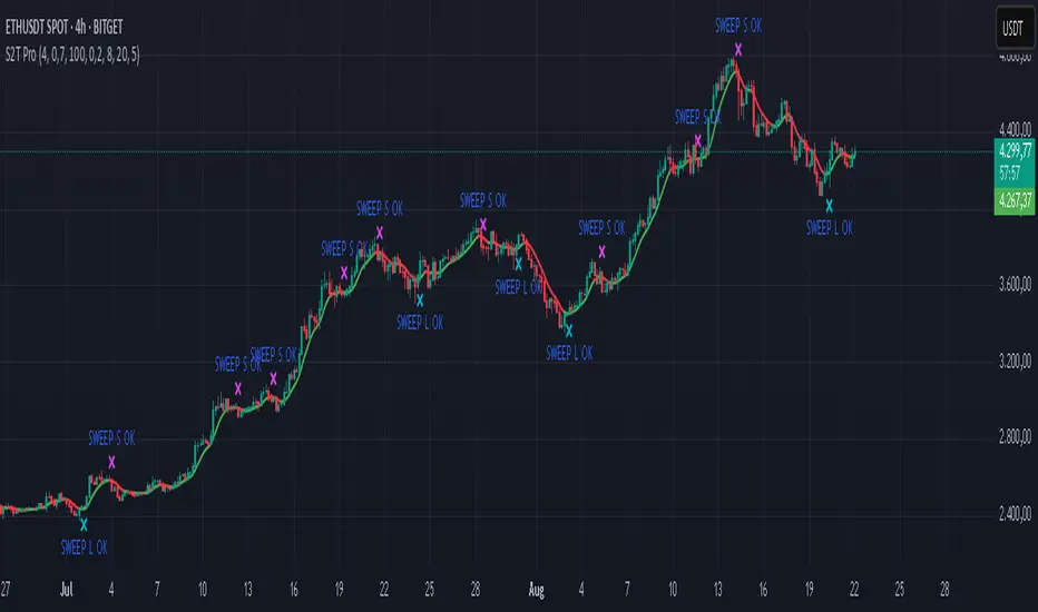
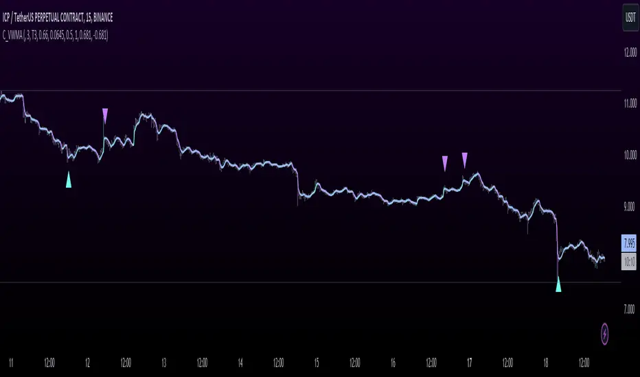
Sweep2Trade Pro [CHE]Sweep2Trade Pro \ — Liquidity Sweep → Trend → Confirmation
Sweep2Trade Pro \ helps you catch high-probability reversals or continuations that start with a liquidity sweep, align with the T3 trend, and finalize with a structure confirmation (BOS). It’s designed to reduce noise, time your entries, and keep you out of weak, chop-driven signals.
What’s a “sweep”?
A liquidity sweep happens when price briefly breaks a prior swing high/low (where many stops sit), triggers those stops, and then snaps back. This “stop-hunt” creates liquidity for bigger players and often precedes a sharp move in the opposite direction if the break fails, or fuels continuation if structure actually shifts.
What’s a BOS (Break of Structure)?
A BOS is a price action event where the market takes out a recent swing level in the trend’s direction, signaling continuation and confirming that structure has shifted (bullish BOS through a recent swing high, bearish BOS through a recent swing low).
How the indicator works (at a glance)
1. Regime Filter (T3 + R²)
T3 Moving Average: A smoother, faster-responding moving average that aims to reduce lag while filtering noise, so trend direction changes are clearer.
R² (Coefficient of Determination): Measures how “linear” the recent price path is (0→1). Higher values = stronger, cleaner trend; lower values = more chop. Used here to allow trades only when trend quality exceeds a user-set threshold.
2. Sweep Detection
Bullish sweep: price pokes below a prior swing low and closes back above it.
Bearish sweep: price pokes above a prior swing high and closes back below it.
Lookback length is configurable.
3. Sequence Lock (built-in FSM)
The script manages state in phases so you don’t jump the gun:
Phase 1: Sweep detected → wait for T3 to turn in the corresponding direction.
Phase 2: T3 direction confirmed → show “SWEEP OK” and wait for final confirmation.
Trade Signal: Only fires if confirmation arrives before a timeout.
4. Confirmation Layer
BOS via wick or close (you choose),
Strong close toward the signal (top/bottom quartile of the candle),
Optional “close above/below T3” condition.
These checks help avoid weak sweeps that immediately fade.
5. Alerts & Visuals
“SWEEP OK” markers show when the sweep + T3 direction align.
Final BUY/SELL arrows appear only when the confirmation layer passes.
Ready-made alert conditions for automation.
What you can do with it
Time reversals after sweeps: Enter when a stop-hunt fades and structure confirms.
Ride continuations: Use BOS with the T3 trend to pyramid or re-enter with structure on your side.
Filter chop: Let R² gate entries to periods with cleaner directional drift.
Automate: Use the included alerts with your platform or webhook setup.
Inputs (key settings)
Regime Filter
T3 Length / Volume Factor: Controls smoothness and responsiveness. Smaller length → faster, more sensitive; higher volume factor → smoother curve.
R² Lookback & Threshold: Length of the linear fit window and the minimum “trend quality” required. Higher thresholds mean fewer, cleaner signals.
Sweep / Sequence
Swing Lookback: How far back to define the “reference” high/low for sweeps.
Timeout: Maximum bars allowed between phases to keep signals fresh.
Restart timeout on Phase 2: Optional safety so entries don’t go stale.
Confirmation
BOS Lookback: Micro-pivot window for structure breaks.
Wick vs Close BOS: Conservative traders may prefer close.
Require close above/below T3: Tightens confirmation with trend alignment.
Practical guide (quick start)
1. Timeframe & markets: Works across majors, indices, and crypto. Start with 5m–1h intraday or 1h–4h swing; adjust R² threshold upward on noisier pairs.
2. Entry recipe (Long):
Bullish sweep of a prior low → T3 turns up → BOS/strong close.
Optional: enable “close above T3” for extra confirmation.
3. Entry recipe (Short): Mirror the above.
4. Stops: Common choices are just beyond the sweep wick (tighter) or past the BOS invalidation (safer).
5. Targets: Previous structural levels, measured move, or a T3 trail (exit when price closes back through T3).
6. Avoid low-quality contexts: If R² is very low, market is likely ranging erratically—skip or widen filters.
Tips & best practices
Context first: The same sweep means different things in a strong trend vs. flat regime; that’s why the T3+R² filter exists.
BOS choice: Wick-based BOS is earlier but noisier; close-based BOS is slower but cleaner. Tune per market.
Backtest -> Forward test: Validate settings per symbol/timeframe; then paper trade before going live.
Risk: Fixed fractional risk with asymmetric R\:R (e.g., 1:1.5–1:3) generally performs better than “all-in” discretionary sizing.
Behind the scenes (for the curious)
T3 is a multi-stage EMA construction that produces a smooth curve with reduced lag versus simple/standard EMAs.
R² is the square of correlation (0–1). Here it’s used as a moving gauge of how well price aligns to a linear path—our “trend quality” dial.
Stop-hunts / sweeps are a recognized microstructure phenomenon where clustered stops provide the liquidity that fuels the next move.
Disclaimer
No indicator guarantees profits. Sweep2Trade Pro \ is a decision aid; always combine with solid risk management and your own judgment. Backtest, forward test, and size responsibly.
The content provided, including all code and materials, is strictly for educational and informational purposes only. It is not intended as, and should not be interpreted as, financial advice, a recommendation to buy or sell any financial instrument, or an offer of any financial product or service. All strategies, tools, and examples discussed are provided for illustrative purposes to demonstrate coding techniques and the functionality of Pine Script within a trading context.
Any results from strategies or tools provided are hypothetical, and past performance is not indicative of future results. Trading and investing involve high risk, including the potential loss of principal, and may not be suitable for all individuals. Before making any trading decisions, please consult with a qualified financial professional to understand the risks involved.
By using this script, you acknowledge and agree that any trading decisions are made solely at your discretion and risk.
Enhance your trading precision and confidence 🚀
Happy trading
Chervolino
Advanced MACD Pro (WhiteStone_Ibrahim) - T3 Themed✨ Advanced MACD Pro (WhiteStone_Ibrahim) - T3 Themed ✨
Take your MACD analysis to the next level with the Advanced MACD Pro - T3 Themed indicator by WhiteStone_Ibrahim! This isn't just another MACD; it's a comprehensive toolkit packed with advanced features, unique T3 integration, and extensive customization options to provide deeper market insights.
Whether you're a seasoned trader or just starting, this indicator offers a versatile and powerful way to analyze momentum, identify trends, and spot potential reversals.
Key Features:
Core MACD Functionality:
Classic MACD Line: Calculated from customizable Fast and Slow EMAs using your chosen source (Close, Open, HLC3, etc.).
Standard Signal Line: EMA of the MACD line, with adjustable length.
Dynamic MACD Line Coloring: Automatically changes color based on whether it's above or below the zero line (positive/negative).
Zero Line: Clearly plotted for reference.
Enhanced MACD Histogram:
Sophisticated Color Coding: The histogram isn't just positive or negative. It intelligently colors based on momentum strength and direction:
Strong Bullish: MACD above signal, histogram increasing.
Weakening Bullish: MACD above signal, histogram decreasing.
Strong Bearish: MACD below signal, histogram decreasing.
Weakening Bearish: MACD below signal, histogram increasing.
Neutral: Default color for other conditions.
Optional Histogram Smoothing: Smooth out the histogram noise using one of five different moving average types: SMA, EMA, WMA, RMA, or the advanced T3 (Tilson T3). Customize smoothing length and T3 vFactor.
🌟 Unique T3 Integration (T3 Themed):
Extra T3 Signal Line (on MACD): An additional, fast-reacting T3 moving average calculated directly from the MACD line. This provides an alternative and often quicker signal.
Customizable T3 length and vFactor.
Dynamic Coloring: The T3 Signal Line changes color (bullish/bearish) based on its crossover with the MACD line, offering clear visual cues.
T3 is also available as a smoothing option for the main histogram (see above).
🔍 Disagreement & Divergence Detection:
Bar/Price Disagreement Markers:
Highlights instances where the price bar's direction (e.g., a bullish candle) contradicts the current MACD momentum (e.g., MACD below its signal line).
Visual markers (circles) appear above/below bars to draw attention to these potential early warnings or confirmations.
Histogram Color Change on Disagreement: Optionally, the histogram can adopt distinct alternative colors during these bar/price disagreements for even clearer visual alerts.
Classic Bullish & Bearish Divergence Detection:
Automatically identifies regular divergences between price action (Higher Highs/Lower Lows) and the MACD line (Lower Highs/Higher Lows).
Customizable pivot lookback periods (left and right bars) for divergence sensitivity.
Plots clear "Bull" and "Bear" labels on the price chart where divergences occur.
🎨 Extensive Customization & Visuals:
Multiple Color Themes: Choose from pre-set themes like 'Dark Mode', 'Light Mode', 'Neon Night', or use 'Default (Current Settings)' to fine-tune every color yourself.
Granular Control (Default Theme): Individually customize colors and thickness for:
MACD Line (positive/negative)
Standard Signal Line
Extra T3 Signal Line (bullish/bearish)
Histogram (all four momentum states + neutral)
Disagreement Markers & Histogram Alt Colors
Divergence Lines/Labels
Zero Line
Toggle Visibility: Easily show or hide the Standard Signal Line and the Extra T3 Signal Line as needed.
🔔 Comprehensive Alert System:
Stay informed of key market events with a wide array of configurable alerts:
MACD Line / Standard Signal Line Crossover
Histogram / Zero Line Crossover
MACD Line / Zero Line Crossover
Bullish Divergence Detected
Bearish Divergence Detected
Bar/Price Disagreement (Bullish & Bearish)
MACD Line / Extra T3 Signal Line Crossover
Each alert can be individually enabled or disabled.
The Advanced MACD Pro - T3 Themed indicator is designed to be your go-to tool for momentum analysis. Its rich feature set empowers you to tailor it to your specific trading style and gain a more nuanced understanding of market dynamics.
Add it to your charts today and experience the difference!
(Developed by WhiteStone_Ibrahim)

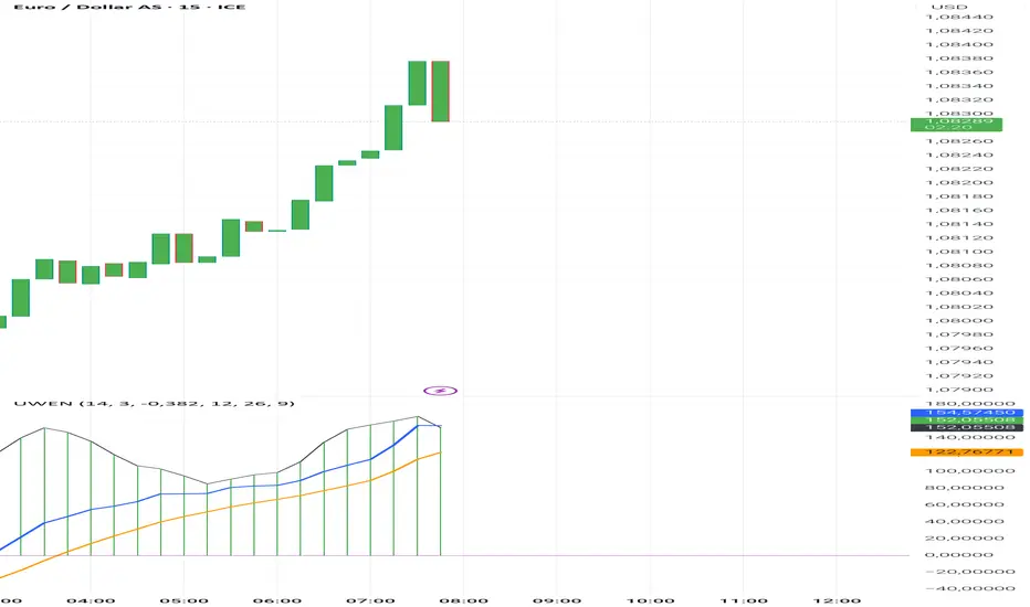
Uwen FX: UWEN StrategyThis Pine Script defines a trading indicator called "Uwen FX: UWEN Strategy" Where ideas coming from Arab Syaukani and modified by Fiki Hafana. It combines a CCI-based T3 Smoothed Indicator with a MACD overlay. Here's a breakdown of what it does:
Key Components of the Script:
1. CCI (Commodity Channel Index) with T3 Smoothing
Uses a T3 smoothing algorithm on the CCI to generate a smoother momentum signal. The smoothing formula is applied iteratively using weighted averages. The final result (xccir) is plotted as a histogram, colored green for bullish signals and red for bearish signals.
2. MACD (Moving Average Convergence Divergence)
The MACD is scaled to match the range of the smoothed CCI for better visualization. Signal Line and MACD Line are plotted if showMACD is enabled. The normalization ensures that MACD values align with the CCI-based indicator.
3. Bar Coloring for Trend Indication
Green bars indicate a positive trend (pos = 1).
Red bars indicate a negative trend (pos = -1).
Blue bars appear when the trend is neutral.
How It Can Be Used:
Buy Signal: When the xccir (smoothed CCI) turns green, indicating bullish momentum.
Sell Signal: When xccir turns red, indicating bearish momentum.
MACD Confirmation: Helps confirm the trend direction by aligning with xccir.
I will add more interesting features if this indicator seems profitable
Normalised T3 Oscillator [BackQuant]Normalised T3 Oscillator
The Normalised T3 Oscillator is an technical indicator designed to provide traders with a refined measure of market momentum by normalizing the T3 Moving Average. This tool was developed to enhance trading decisions by smoothing price data and reducing market noise, allowing for clearer trend recognition and potential signal generation. Below is a detailed breakdown of the Normalised T3 Oscillator, its methodology, and its application in trading scenarios.
1. Conceptual Foundation and Definition of T3
The T3 Moving Average, originally proposed by Tim Tillson, is renowned for its smoothness and responsiveness, achieved through a combination of multiple Exponential Moving Averages and a volume factor. The Normalised T3 Oscillator extends this concept by normalizing these values to oscillate around a central zero line, which aids in highlighting overbought and oversold conditions.
2. Normalization Process
Normalization in this context refers to the adjustment of the T3 values to ensure that the oscillator provides a standard range of output. This is accomplished by calculating the lowest and highest values of the T3 over a user-defined period and scaling the output between -0.5 to +0.5. This process not only aids in standardizing the indicator across different securities and time frames but also enhances comparative analysis.
3. Integration of the Oscillator and Moving Average
A unique feature of the Normalised T3 Oscillator is the inclusion of a secondary smoothing mechanism via a moving average of the oscillator itself, selectable from various types such as SMA, EMA, and more. This moving average acts as a signal line, providing potential buy or sell triggers when the oscillator crosses this line, thus offering dual layers of analysis—momentum and trend confirmation.
4. Visualization and User Interaction
The indicator is designed with user interaction in mind, featuring customizable parameters such as the length of the T3, normalization period, and type of moving average used for signals. Additionally, the oscillator is plotted with a color-coded scheme that visually represents different strength levels of the market conditions, enhancing readability and quick decision-making.
5. Practical Applications and Strategy Integration
Traders can leverage the Normalised T3 Oscillator in various trading strategies, including trend following, counter-trend plays, and as a component of a broader trading system. It is particularly useful in identifying turning points in the market or confirming ongoing trends. The clear visualization and customizable nature of the oscillator facilitate its adaptation to different trading styles and market environments.
6. Advanced Features and Customization
Further enhancing its utility, the indicator includes options such as painting candles according to the trend, showing static levels for quick reference, and alerts for crossover and crossunder events, which can be integrated into automated trading systems. These features allow for a high degree of personalization, enabling traders to mold the tool according to their specific trading preferences and risk management requirements.
7. Theoretical Justification and Empirical Usage
The use of the T3 smoothing mechanism combined with normalization is theoretically sound, aiming to reduce lag and false signals often associated with traditional moving averages. The practical effectiveness of the Normalised T3 Oscillator should be validated through rigorous backtesting and adjustment of parameters to match historical market conditions and volatility.
8. Conclusion and Utility in Market Analysis
Overall, the Normalised T3 Oscillator by BackQuant stands as a sophisticated tool for market analysis, providing traders with a dynamic and adaptable approach to gauging market momentum. Its development is rooted in the understanding of technical nuances and the demand for a more stable, responsive, and customizable trading indicator.
Thus following all of the key points here are some sample backtests on the 1D Chart
Disclaimer: Backtests are based off past results, and are not indicative of the future.
INDEX:BTCUSD
INDEX:ETHUSD
BINANCE:SOLUSD

Leading T3Hello Fellas,
Here, I applied a special technique of John F. Ehlers to make lagging indicators leading. The T3 itself is usually not realling the classic lagging indicator, so it is not really needed, but I still publish this indicator to demonstrate this technique of Ehlers applied on a simple indicator.
The indicator does not repaint.
In the following picture you can see a comparison of normal T3 (purple) compared to a 2-bar "leading" T3 (gradient):
The range of the gradient is:
Bottom Value: the lowest slope of the last 100 bars -> green
Top Value: the highest slope of the last 100 bars -> purple
Ehlers Special Technique
John Ehlers did develop methods to make lagging indicators leading or predictive. One of these methods is the Predictive Moving Average, which he introduced in his book “Rocket Science for Traders”. The concept is to take a difference of a lagging line from the original function to produce a leading function.
The idea is to extend this concept to moving averages. If you take a 7-bar Weighted Moving Average (WMA) of prices, that average lags the prices by 2 bars. If you take a 7-bar WMA of the first average, this second average is delayed another 2 bars. If you take the difference between the two averages and add that difference to the first average, the result should be a smoothed line of the original price function with no lag.
T3
To compute the T3 moving average, it involves a triple smoothing process using exponential moving averages. Here's how it works:
Calculate the first exponential moving average (EMA1) of the price data over a specific period 'n.'
Calculate the second exponential moving average (EMA2) of EMA1 using the same period 'n.'
Calculate the third exponential moving average (EMA3) of EMA2 using the same period 'n.'
The formula for the T3 moving average is as follows:
T3 = 3 * (EMA1) - 3 * (EMA2) + (EMA3)
By applying this triple smoothing process, the T3 moving average is intended to offer reduced noise and improved responsiveness to price trends. It achieves this by incorporating multiple time frames of the exponential moving averages, resulting in a more accurate representation of the underlying price action.
Thanks for checking this out and give a boost, if you enjoyed the content.
Best regards,
simwai
---
Credits to @loxx

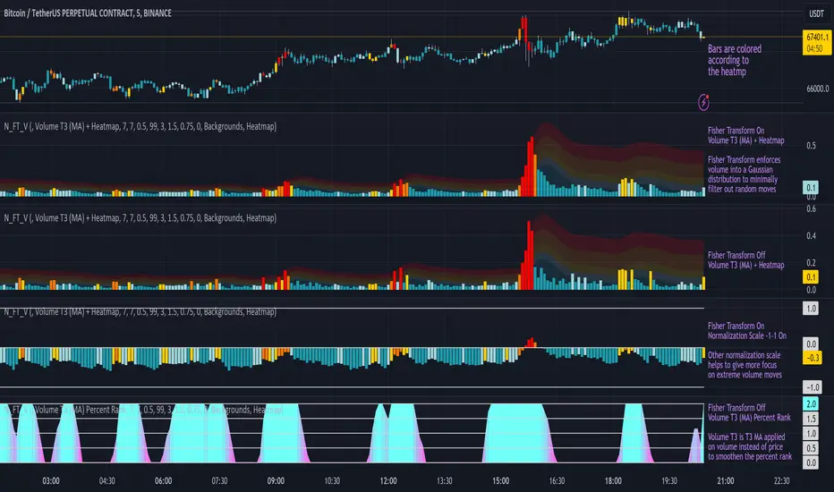
Normalized Fisher Transformed VolumeGreetings Traders,
I am thrilled to introduce a game-changing tool that I've passionately developed to enhance your trading precision – the Normalized Fisher Transformed Volume indicator. Let's dive into the specifics and explore how this tool can empower you in the markets.
Unlocking Trading Precision:
Normalization and Transformation:
Normalize raw volume data to ensure a consistent scale for analysis.
The Fisher Transformation converts normalized volume data into a Gaussian distribution, providing enhanced insights into trend dynamics.
Flexible Modes for Tailored Strategies:
Choose from three distinct modes:
Volume T3 (MA) + Heatmap: Identify trends with T3 Moving Average and visualize volume strength with Heatmap.
Volume Percent Rank: Evaluate the position of current volume relative to historical data.
Volume T3 (MA) Percent Rank: Combine T3 Moving Average with percentile ranking for a comprehensive analysis.
Heatmap Visualization for Quick Insights:
Heatmap Zones and Lines visually represent volume strength relative to historical data.
Customize threshold multipliers and color options for precise Heatmap interpretation.
T3 Moving Average Integration:
Smoothed representation of volume trends with the T3 Moving Average enhances trend identification.
Percent Rank Analysis for Context:
Gauge the position of normalized volume within historical context using Percent Rank analysis.
User-Friendly Customization:
Easily adjust parameters such as length, T3 Moving Average length, Heatmap standard deviation length, and threshold multipliers.
Intuitive interface with colored bars and customizable background options for personalized analysis.
How to Use Effectively:
Mode Selection:
Identify your preferred trading strategy and select the mode that aligns with your approach.
Parameter Adjustment:
Fine-tune the indicator by adjusting parameters to match your preferred trading style.
Interpret Heatmap and T3 Analysis:
Leverage Heatmap and T3 Moving Average analysis to spot potential trend reversals, overbought/oversold conditions, and market sentiment shifts.
Conclusion:
The Normalized Fisher Transformed Volume indicator is not just a tool; it's your key to unlocking precision in trading. Crafted by Simwai, this indicator offers unique insights tailored to your specific trading needs. Dive in, explore its features, experiment with parameters, and let it guide you to more informed and precise trading decisions.
Trade wisely and prosper,
simwai
EMA-Deviation-Corrected T3 [Loxx]EMA-Deviation-Corrected T3 is a T3 moving average that uses EMA deviation correcting to produce signals. This comes via the beloved genius Mladen.
The origin of the correcting algorithm can be attributed to Dr. Alexander Uhl, who developed a method to filter the moving average and identify signals. Originally, this method utilized standard deviation as a measure to correct the average values.
However, the current indicator in question employs a modified version of the correcting method. Instead of using standard deviation for calculation, it uses EMA deviation, which stands for Exponential Moving Average deviation. The idea behind using EMA deviation is two-fold:
Efficiency: EMA deviation can be calculated faster than standard deviation, resulting in more efficient code execution.
Signal Reduction: Surprisingly, this modified "correcting" approach generates fewer signals compared to using standard deviation. This is because EMA deviation is more responsive to price changes, making the correcting process less sensitive to whipsaws or false signals.
What is T3?
The T3 moving average, short for "Tim Tillson's Triple Exponential Moving Average," is a technical indicator used in financial markets and technical analysis to smooth out price data over a specific period. It was developed by Tim Tillson, a software project manager at Hewlett-Packard, with expertise in Mathematics and Computer Science.
The T3 moving average is an enhancement of the traditional Exponential Moving Average (EMA) and aims to overcome some of its limitations. The primary goal of the T3 moving average is to provide a smoother representation of price trends while minimizing lag compared to other moving averages like Simple Moving Average (SMA), Weighted Moving Average (WMA), or EMA.
To compute the T3 moving average, it involves a triple smoothing process using exponential moving averages. Here's how it works:
Calculate the first exponential moving average (EMA1) of the price data over a specific period 'n.'
Calculate the second exponential moving average (EMA2) of EMA1 using the same period 'n.'
Calculate the third exponential moving average (EMA3) of EMA2 using the same period 'n.'
The formula for the T3 moving average is as follows:
T3 = 3 * (EMA1) - 3 * (EMA2) + (EMA3)
By applying this triple smoothing process, the T3 moving average is intended to offer reduced noise and improved responsiveness to price trends. It achieves this by incorporating multiple time frames of the exponential moving averages, resulting in a more accurate representation of the underlying price action.
Included
Bar coloring
Signals
Alerts
Loxx's Expanded Source Types

Tillson T3 Moving Average - ScreenerScreener version of Tillson T3 Moving Average:
The T3 Moving Average generally produces entry signals similar to other moving averages and, thus, is mainly traded in the same manner. Here are several assumptions:
Suppose the price action is above the T3 Moving Average, and the indicator is upward. In that case, we have a bullish trend and should only enter long trades (advisable for novice/intermediate traders). If the price is below the T3 Moving Average and edging lower, we have a bearish trend and should limit entries to short.
About Screener Panel:
Users can explore 20 different and user-defined tickers, which can be changed from the SETTINGS (shares, crypto, commodities...) on this screener version.
The screener panel shows up right after the bars on the right side of the chart.
Tickers seen in green are the ones that are in an uptrend, according to T3.
The ones that appear in red are those in the SELL signal, in a downtrend.
The numbers in front of each Ticker indicate how many bars passed after the last BUY or SELL signal of T3.
For example, according to the indicator, when BTCUSDT appears (3) in GREEN, Bitcoin switched to a BUY signal 3 bars ago.
-In this screener version of Tillson T3 Moving Average, users can define the number of demanded tickers (symbols) from 1 to 20 by checking the relevant boxes on the settings tab.
-All selected tickers can be screened in different timeframes.
-Also, different timeframes of the same Ticker can be screened.
IMPORTANT NOTICE:
Screener shows the results in 2 different logic:
-Screener shows the information about the color changes of the T3 Moving Average with default settings.
-Users can check the "Change Screener to show T3 & Price Flips" button to activate the screener giving information about price flips.
If this option is preferred, users are advised to enlarge the length to have better signals.

Regularized-Moving-Average Oscillator SuiteThe Regularized-MA Oscillator Suite is a versatile indicator that transforms any moving average into an oscillator. It comprises up to 13 different moving average types, including KAMA, T3, and ALMA. This indicator serves as a valuable tool for both trend following and mean reversion strategies, providing traders and investors with enhanced insights into market dynamics.
Methodology:
The Regularized MA Oscillator Suite calculates the moving average (MA) based on user-defined parameters such as length, moving average type, and custom smoothing factors. It then derives the mean and standard deviation of the MA using a normalized period. Finally, it computes the Z-Score by subtracting the mean from the MA and dividing it by the standard deviation.
KAMA (Kaufman's Adaptive Moving Average):
KAMA is a unique moving average type that dynamically adjusts its smoothing period based on market volatility. It adapts to changing market conditions, providing a smoother response during periods of low volatility and a quicker response during periods of high volatility. This allows traders to capture trends effectively while reducing noise.
T3 (Tillson's Exponential Moving Average):
T3 is an exponential moving average that incorporates additional smoothing techniques to reduce lag and provide a more responsive indicator. It aims to maintain a balance between responsiveness and smoothness, allowing traders to identify trend reversals with greater accuracy.
ALMA (Arnaud Legoux Moving Average):
ALMA is a moving average type that utilizes a combination of linear regression and exponential moving average techniques. It offers a unique way of calculating the moving average by providing a smoother and more accurate representation of price trends. ALMA reduces lag and noise, enabling traders to identify trend changes and potential entry or exit points more effectively.
Z-Score:
The Z-Score calculation in the Regularized-MA Oscillator Suite standardizes the values of the moving average. It measures the deviation of each data point from the mean in terms of standard deviations. By normalizing the moving average through the Z-Score, the indicator enables traders to assess the relative position of price in relation to its mean and volatility. This information can be valuable for identifying overbought and oversold conditions, as well as potential trend reversals.
Utility:
The Regularized-MA Oscillator Suite with its unique moving average types and Z-Score calculation offers traders and investors powerful analytical tools. It can be used for trend following strategies by analyzing the oscillator's position relative to the midline. Traders can also employ it as a mean reversion tool by identifying peak values above user-defined deviations. These features assist in identifying potential entry and exit points, enhancing trading decisions and market analysis.
Key Features:
Variety of 13 MA types.
Potential reversal point bubbles.
Bar coloring methods - Trend (Midline cross), Extremities, Reversions, Slope
Example Charts:

T3 JMA KAMA VWMAEnhancing Trading Performance with T3 JMA KAMA VWMA Indicator
Introduction
In the dynamic world of trading, staying ahead of market trends and capitalizing on volume-driven opportunities can greatly influence trading performance. To address this, we have developed the T3 JMA KAMA VWMA Indicator, an innovative tool that modifies the traditional Volume Weighted Moving Average (VWMA) formula to increase responsiveness and exploit high-volume market conditions for optimal position entry. This article delves into the idea behind this modification and how it can benefit traders seeking to gain an edge in the market.
The Idea Behind the Modification
The core concept behind modifying the VWMA formula is to leverage more responsive moving averages (MAs) that align with high-volume market activity. Traditional VWMA utilizes the Simple Moving Average (SMA) as the basis for calculating the weighted average. While the SMA is effective in providing a smoothed perspective of price movements, it may lack the desired responsiveness to capitalize on short-term volume-driven opportunities.
To address this limitation, our T3 JMA KAMA VWMA Indicator incorporates three advanced moving averages: T3, JMA, and KAMA. These MAs offer enhanced responsiveness, allowing traders to react swiftly to changing market conditions influenced by volume.
T3 (T3 New and T3 Normal):
The T3 moving average, one of the components of our indicator, applies a proprietary algorithm that provides smoother and more responsive trend signals. By utilizing T3, we ensure that the VWMA calculation aligns with the dynamic nature of high-volume markets, enabling traders to capture price movements accurately.
JMA (Jurik Moving Average):
The JMA component further enhances the indicator's responsiveness by incorporating phase shifting and power adjustment. This adaptive approach ensures that the moving average remains sensitive to changes in volume and price dynamics. As a result, traders can identify turning points and anticipate potential trend reversals, precisely timing their position entries.
KAMA (Kaufman's Adaptive Moving Average):
KAMA is an adaptive moving average designed to dynamically adjust its sensitivity based on market conditions. By incorporating KAMA into our VWMA modification, we ensure that the moving average adapts to varying volume levels and captures the essence of volume-driven price movements. Traders can confidently enter positions during periods of high trading volume, aligning their strategies with market activity.
Benefits and Usage
The modified T3 JMA KAMA VWMA Indicator offers several advantages to traders looking to exploit high-volume market conditions for position entry:
Increased Responsiveness: By incorporating more responsive moving averages, the indicator enables traders to react quickly to changes in volume and capture short-term opportunities more effectively.
Enhanced Entry Timing: The modified VWMA aligns with high-volume periods, allowing traders to enter positions precisely during price movements influenced by significant trading activity.
Improved Accuracy: The combination of T3, JMA, and KAMA within the VWMA formula enhances the accuracy of trend identification, reversals, and overall market analysis.
Comprehensive Market Insights: The T3 JMA KAMA VWMA Indicator provides a holistic view of market conditions by considering both price and volume dynamics. This comprehensive perspective helps traders make informed decisions.
Analysis and Interpretation
The modified VWMA formula with T3, JMA, and KAMA offers traders a valuable tool for analyzing volume-driven market conditions. By incorporating these advanced moving averages into the VWMA calculation, the indicator becomes more responsive to changes in volume, potentially providing deeper insights into price movements.
When analyzing the modified VWMA, it is essential to consider the following points:
Identifying High-Volume Periods:
The modified VWMA is designed to capture price movements during high-volume periods. Traders can use this indicator to identify potential market trends and determine whether significant trading activity is driving price action. By focusing on these periods, traders may gain a better understanding of the market sentiment and adjust their strategies accordingly.
Confirmation of Trend Strength:
The modified VWMA can serve as a confirmation tool for assessing the strength of a trend. When the VWMA line aligns with the overall trend direction, it suggests that the current price movement is supported by volume. This confirmation can provide traders with additional confidence in their analysis and help them make more informed trading decisions.
Potential Entry and Exit Points:
One of the primary purposes of the modified VWMA is to assist traders in identifying potential entry and exit points. By capturing volume-driven price movements, the indicator can highlight areas where market participants are actively participating, indicating potential opportunities for opening or closing positions. Traders can use this information in conjunction with other technical analysis tools to develop comprehensive trading strategies.
Interpretation of Angle and Gradient:
The modified VWMA incorporates an angle calculation and color gradient to further enhance interpretation. The angle of the VWMA line represents the slope of the indicator, providing insights into the momentum of price movements. A steep angle indicates strong momentum, while a shallow angle suggests a slowdown. The color gradient helps visualize this angle, with green indicating bullish momentum and purple indicating bearish momentum.
Conclusion
By modifying the VWMA formula to incorporate the T3, JMA, and KAMA moving averages, the T3 JMA KAMA VWMA Indicator offers traders an innovative tool to exploit high-volume market conditions for optimal position entry. This modification enhances responsiveness, improves timing, and provides comprehensive market insights.
Enjoy checking it out!
---
Credits to:
◾ @cheatcountry – Hann Window Smoothing
◾ @loxx – T3
◾ @everget – JMA
T3 OscillatorTL;DR - An Oscillator based on T3 moving average
The T3 moving average is a well known moving average created by Tim TIllson. Oscillator values are created by using the simple formula "source (close by default) - T3 moving average". Tim Tillson used a "volume factor" of 0.7 in his original T3 calculation. I changed this value to 0.618 and added the option to change it if needed/wanted. I also added alarms for zero line crossing upwards and downward, a smoothing option and custom time frames.
Compared to other oscillators like TSI, MACD etc. I observed better signals, especially in trending market situations, from the T3 oscillator (I tested Forex and Crypto).
Usage is simple: If the oscillator is above 0 it indicates a bearish trend. If below 0 it indicates a bullish trend. -> Really simple to use. However it can also be used to determine micro trends and reversals when combined with price action analysis. To keeps things simple I have not added a moving average like many other oscillators because I think it is confusing and does not help (in this particular case).
P.S. I haven't found a T3 oscillator on Trading View. Code is free - do whatever you want with it ;)

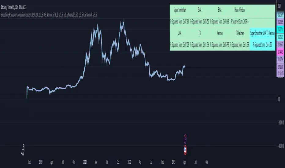
Smoothing R-Squared ComparisonIntroduction
Heyo guys, here I made a comparison between my favorised smoothing algorithms.
I chose the R-Squared value as rating factor to accomplish the comparison.
The indicator is non-repainting.
Description
In technical analysis, traders often use moving averages to smooth out the noise in price data and identify trends. While moving averages are a useful tool, they can also obscure important information about the underlying relationship between the price and the smoothed price.
One way to evaluate this relationship is by calculating the R-squared value, which represents the proportion of the variance in the price that can be explained by the smoothed price in a linear regression model.
This PineScript code implements a smoothing R-squared comparison indicator.
It provides a comparison of different smoothing techniques such as Kalman filter, T3, JMA, EMA, SMA, Super Smoother and some special combinations of them.
The Kalman filter is a mathematical algorithm that uses a series of measurements observed over time, containing statistical noise and other inaccuracies, and produces estimates of unknown variables that tend to be more accurate than those based on a single measurement.
The input parameters for the Kalman filter include the process noise covariance and the measurement noise covariance, which help to adjust the sensitivity of the filter to changes in the input data.
The T3 smoothing technique is a popular method used in technical analysis to remove noise from a signal.
The input parameters for the T3 smoothing method include the length of the window used for smoothing, the type of smoothing used (Normal or New), and the smoothing factor used to adjust the sensitivity to changes in the input data.
The JMA smoothing technique is another popular method used in technical analysis to remove noise from a signal.
The input parameters for the JMA smoothing method include the length of the window used for smoothing, the phase used to shift the input data before applying the smoothing algorithm, and the power used to adjust the sensitivity of the JMA to changes in the input data.
The EMA and SMA techniques are also popular methods used in technical analysis to remove noise from a signal.
The input parameters for the EMA and SMA techniques include the length of the window used for smoothing.
The indicator displays a comparison of the R-squared values for each smoothing technique, which provides an indication of how well the technique is fitting the data.
Higher R-squared values indicate a better fit. By adjusting the input parameters for each smoothing technique, the user can compare the effectiveness of different techniques in removing noise from the input data.
Usage
You can use it to find the best fitting smoothing method for the timeframe you usually use.
Just apply it on your preferred timeframe and look for the highlighted table cell.
Conclusion
It seems like the T3 works best on timeframes under 4H.
There's where I am active, so I will use this one more in the future.
Thank you for checking this out. Enjoy your day and leave me a like or comment. 🧙♂️
---
Credits to:
▪@loxx – T3
▪@balipour – Super Smoother
▪ChatGPT – Wrote 80 % of this article and helped with the research
PA-Adaptive T3 Loxxer [Loxx]PA-Adaptive T3 Loxxer is a Loxxer indicator that is Phase Accumulation Cycle adaptive and uses T3 moving average for smoothing instead of the typical SMA or EMA . this allows for smoother signals by reducing noise.
What is Loxxer?
The Loxxer indicator is a technical analysis tool that compares the most recent maximum and minimum prices to the previous period's equivalent price to measure the demand of the underlying asset.
What is the Phase Accumulation Cycle?
The phase accumulation method of computing the dominant cycle is perhaps the easiest to comprehend. In this technique, we measure the phase at each sample by taking the arctangent of the ratio of the quadrature component to the in-phase component. A delta phase is generated by taking the difference of the phase between successive samples. At each sample we can then look backwards, adding up the delta phases.When the sum of the delta phases reaches 360 degrees, we must have passed through one full cycle, on average.The process is repeated for each new sample.
The phase accumulation method of cycle measurement always uses one full cycle’s worth of historical data.This is both an advantage and a disadvantage.The advantage is the lag in obtaining the answer scales directly with the cycle period.That is, the measurement of a short cycle period has less lag than the measurement of a longer cycle period. However, the number of samples used in making the measurement means the averaging period is variable with cycle period. longer averaging reduces the noise level compared to the signal.Therefore, shorter cycle periods necessarily have a higher out- put signal-to-noise ratio.
Included
Bar coloring
Signals
Alerts
Loxx's Expanded Source Types
Divergences

STD-Adaptive T3 [Loxx]STD-Adaptive T3 is a standard deviation adaptive T3 moving average filter. This indicator acts more like a trend overlay indicator with gradient coloring.
What is the T3 moving average?
Better Moving Averages Tim Tillson
November 1, 1998
Tim Tillson is a software project manager at Hewlett-Packard, with degrees in Mathematics and Computer Science. He has privately traded options and equities for 15 years.
Introduction
"Digital filtering includes the process of smoothing, predicting, differentiating, integrating, separation of signals, and removal of noise from a signal. Thus many people who do such things are actually using digital filters without realizing that they are; being unacquainted with the theory, they neither understand what they have done nor the possibilities of what they might have done."
This quote from R. W. Hamming applies to the vast majority of indicators in technical analysis . Moving averages, be they simple, weighted, or exponential, are lowpass filters; low frequency components in the signal pass through with little attenuation, while high frequencies are severely reduced.
"Oscillator" type indicators (such as MACD , Momentum, Relative Strength Index ) are another type of digital filter called a differentiator.
Tushar Chande has observed that many popular oscillators are highly correlated, which is sensible because they are trying to measure the rate of change of the underlying time series, i.e., are trying to be the first and second derivatives we all learned about in Calculus.
We use moving averages (lowpass filters) in technical analysis to remove the random noise from a time series, to discern the underlying trend or to determine prices at which we will take action. A perfect moving average would have two attributes:
It would be smooth, not sensitive to random noise in the underlying time series. Another way of saying this is that its derivative would not spuriously alternate between positive and negative values.
It would not lag behind the time series it is computed from. Lag, of course, produces late buy or sell signals that kill profits.
The only way one can compute a perfect moving average is to have knowledge of the future, and if we had that, we would buy one lottery ticket a week rather than trade!
Having said this, we can still improve on the conventional simple, weighted, or exponential moving averages. Here's how:
Two Interesting Moving Averages
We will examine two benchmark moving averages based on Linear Regression analysis.
In both cases, a Linear Regression line of length n is fitted to price data.
I call the first moving average ILRS, which stands for Integral of Linear Regression Slope. One simply integrates the slope of a linear regression line as it is successively fitted in a moving window of length n across the data, with the constant of integration being a simple moving average of the first n points. Put another way, the derivative of ILRS is the linear regression slope. Note that ILRS is not the same as a SMA ( simple moving average ) of length n, which is actually the midpoint of the linear regression line as it moves across the data.
We can measure the lag of moving averages with respect to a linear trend by computing how they behave when the input is a line with unit slope. Both SMA (n) and ILRS(n) have lag of n/2, but ILRS is much smoother than SMA .
Our second benchmark moving average is well known, called EPMA or End Point Moving Average. It is the endpoint of the linear regression line of length n as it is fitted across the data. EPMA hugs the data more closely than a simple or exponential moving average of the same length. The price we pay for this is that it is much noisier (less smooth) than ILRS, and it also has the annoying property that it overshoots the data when linear trends are present.
However, EPMA has a lag of 0 with respect to linear input! This makes sense because a linear regression line will fit linear input perfectly, and the endpoint of the LR line will be on the input line.
These two moving averages frame the tradeoffs that we are facing. On one extreme we have ILRS, which is very smooth and has considerable phase lag. EPMA has 0 phase lag, but is too noisy and overshoots. We would like to construct a better moving average which is as smooth as ILRS, but runs closer to where EPMA lies, without the overshoot.
A easy way to attempt this is to split the difference, i.e. use (ILRS(n)+EPMA(n))/2. This will give us a moving average (call it IE /2) which runs in between the two, has phase lag of n/4 but still inherits considerable noise from EPMA. IE /2 is inspirational, however. Can we build something that is comparable, but smoother? Figure 1 shows ILRS, EPMA, and IE /2.
Filter Techniques
Any thoughtful student of filter theory (or resolute experimenter) will have noticed that you can improve the smoothness of a filter by running it through itself multiple times, at the cost of increasing phase lag.
There is a complementary technique (called twicing by J.W. Tukey) which can be used to improve phase lag. If L stands for the operation of running data through a low pass filter, then twicing can be described by:
L' = L(time series) + L(time series - L(time series))
That is, we add a moving average of the difference between the input and the moving average to the moving average. This is algebraically equivalent to:
2L-L(L)
This is the Double Exponential Moving Average or DEMA , popularized by Patrick Mulloy in TASAC (January/February 1994).
In our taxonomy, DEMA has some phase lag (although it exponentially approaches 0) and is somewhat noisy, comparable to IE /2 indicator.
We will use these two techniques to construct our better moving average, after we explore the first one a little more closely.
Fixing Overshoot
An n-day EMA has smoothing constant alpha=2/(n+1) and a lag of (n-1)/2.
Thus EMA (3) has lag 1, and EMA (11) has lag 5. Figure 2 shows that, if I am willing to incur 5 days of lag, I get a smoother moving average if I run EMA (3) through itself 5 times than if I just take EMA (11) once.
This suggests that if EPMA and DEMA have 0 or low lag, why not run fast versions (eg DEMA (3)) through themselves many times to achieve a smooth result? The problem is that multiple runs though these filters increase their tendency to overshoot the data, giving an unusable result. This is because the amplitude response of DEMA and EPMA is greater than 1 at certain frequencies, giving a gain of much greater than 1 at these frequencies when run though themselves multiple times. Figure 3 shows DEMA (7) and EPMA(7) run through themselves 3 times. DEMA^3 has serious overshoot, and EPMA^3 is terrible.
The solution to the overshoot problem is to recall what we are doing with twicing:
DEMA (n) = EMA (n) + EMA (time series - EMA (n))
The second term is adding, in effect, a smooth version of the derivative to the EMA to achieve DEMA . The derivative term determines how hot the moving average's response to linear trends will be. We need to simply turn down the volume to achieve our basic building block:
EMA (n) + EMA (time series - EMA (n))*.7;
This is algebraically the same as:
EMA (n)*1.7-EMA( EMA (n))*.7;
I have chosen .7 as my volume factor, but the general formula (which I call "Generalized Dema") is:
GD (n,v) = EMA (n)*(1+v)-EMA( EMA (n))*v,
Where v ranges between 0 and 1. When v=0, GD is just an EMA , and when v=1, GD is DEMA . In between, GD is a cooler DEMA . By using a value for v less than 1 (I like .7), we cure the multiple DEMA overshoot problem, at the cost of accepting some additional phase delay. Now we can run GD through itself multiple times to define a new, smoother moving average T3 that does not overshoot the data:
T3(n) = GD ( GD ( GD (n)))
In filter theory parlance, T3 is a six-pole non-linear Kalman filter. Kalman filters are ones which use the error (in this case (time series - EMA (n)) to correct themselves. In Technical Analysis , these are called Adaptive Moving Averages; they track the time series more aggressively when it is making large moves.
Included
Bar coloring
Loxx's Expanded Source Types

Softmax Normalized T3 Histogram [Loxx]Softmax Normalized T3 Histogram is a T3 moving average that is morphed into a normalized oscillator from -1 to 1.
What is the Softmax function?
The softmax function, also known as softargmax: or normalized exponential function, converts a vector of K real numbers into a probability distribution of K possible outcomes. It is a generalization of the logistic function to multiple dimensions, and used in multinomial logistic regression. The softmax function is often used as the last activation function of a neural network to normalize the output of a network to a probability distribution over predicted output classes, based on Luce's choice axiom.
What is the T3 moving average?
Better Moving Averages Tim Tillson
November 1, 1998
Tim Tillson is a software project manager at Hewlett-Packard, with degrees in Mathematics and Computer Science. He has privately traded options and equities for 15 years.
Introduction
"Digital filtering includes the process of smoothing, predicting, differentiating, integrating, separation of signals, and removal of noise from a signal. Thus many people who do such things are actually using digital filters without realizing that they are; being unacquainted with the theory, they neither understand what they have done nor the possibilities of what they might have done."
This quote from R. W. Hamming applies to the vast majority of indicators in technical analysis . Moving averages, be they simple, weighted, or exponential, are lowpass filters; low frequency components in the signal pass through with little attenuation, while high frequencies are severely reduced.
"Oscillator" type indicators (such as MACD , Momentum, Relative Strength Index ) are another type of digital filter called a differentiator.
Tushar Chande has observed that many popular oscillators are highly correlated, which is sensible because they are trying to measure the rate of change of the underlying time series, i.e., are trying to be the first and second derivatives we all learned about in Calculus.
We use moving averages (lowpass filters) in technical analysis to remove the random noise from a time series, to discern the underlying trend or to determine prices at which we will take action. A perfect moving average would have two attributes:
It would be smooth, not sensitive to random noise in the underlying time series. Another way of saying this is that its derivative would not spuriously alternate between positive and negative values.
It would not lag behind the time series it is computed from. Lag, of course, produces late buy or sell signals that kill profits.
The only way one can compute a perfect moving average is to have knowledge of the future, and if we had that, we would buy one lottery ticket a week rather than trade!
Having said this, we can still improve on the conventional simple, weighted, or exponential moving averages. Here's how:
Two Interesting Moving Averages
We will examine two benchmark moving averages based on Linear Regression analysis.
In both cases, a Linear Regression line of length n is fitted to price data.
I call the first moving average ILRS, which stands for Integral of Linear Regression Slope. One simply integrates the slope of a linear regression line as it is successively fitted in a moving window of length n across the data, with the constant of integration being a simple moving average of the first n points. Put another way, the derivative of ILRS is the linear regression slope. Note that ILRS is not the same as a SMA ( simple moving average ) of length n, which is actually the midpoint of the linear regression line as it moves across the data.
We can measure the lag of moving averages with respect to a linear trend by computing how they behave when the input is a line with unit slope. Both SMA (n) and ILRS(n) have lag of n/2, but ILRS is much smoother than SMA .
Our second benchmark moving average is well known, called EPMA or End Point Moving Average. It is the endpoint of the linear regression line of length n as it is fitted across the data. EPMA hugs the data more closely than a simple or exponential moving average of the same length. The price we pay for this is that it is much noisier (less smooth) than ILRS, and it also has the annoying property that it overshoots the data when linear trends are present.
However, EPMA has a lag of 0 with respect to linear input! This makes sense because a linear regression line will fit linear input perfectly, and the endpoint of the LR line will be on the input line.
These two moving averages frame the tradeoffs that we are facing. On one extreme we have ILRS, which is very smooth and has considerable phase lag. EPMA has 0 phase lag, but is too noisy and overshoots. We would like to construct a better moving average which is as smooth as ILRS, but runs closer to where EPMA lies, without the overshoot.
A easy way to attempt this is to split the difference, i.e. use (ILRS(n)+EPMA(n))/2. This will give us a moving average (call it IE /2) which runs in between the two, has phase lag of n/4 but still inherits considerable noise from EPMA. IE /2 is inspirational, however. Can we build something that is comparable, but smoother? Figure 1 shows ILRS, EPMA, and IE /2.
Filter Techniques
Any thoughtful student of filter theory (or resolute experimenter) will have noticed that you can improve the smoothness of a filter by running it through itself multiple times, at the cost of increasing phase lag.
There is a complementary technique (called twicing by J.W. Tukey) which can be used to improve phase lag. If L stands for the operation of running data through a low pass filter, then twicing can be described by:
L' = L(time series) + L(time series - L(time series))
That is, we add a moving average of the difference between the input and the moving average to the moving average. This is algebraically equivalent to:
2L-L(L)
This is the Double Exponential Moving Average or DEMA , popularized by Patrick Mulloy in TASAC (January/February 1994).
In our taxonomy, DEMA has some phase lag (although it exponentially approaches 0) and is somewhat noisy, comparable to IE /2 indicator.
We will use these two techniques to construct our better moving average, after we explore the first one a little more closely.
Fixing Overshoot
An n-day EMA has smoothing constant alpha=2/(n+1) and a lag of (n-1)/2.
Thus EMA (3) has lag 1, and EMA (11) has lag 5. Figure 2 shows that, if I am willing to incur 5 days of lag, I get a smoother moving average if I run EMA (3) through itself 5 times than if I just take EMA (11) once.
This suggests that if EPMA and DEMA have 0 or low lag, why not run fast versions (eg DEMA (3)) through themselves many times to achieve a smooth result? The problem is that multiple runs though these filters increase their tendency to overshoot the data, giving an unusable result. This is because the amplitude response of DEMA and EPMA is greater than 1 at certain frequencies, giving a gain of much greater than 1 at these frequencies when run though themselves multiple times. Figure 3 shows DEMA (7) and EPMA(7) run through themselves 3 times. DEMA^3 has serious overshoot, and EPMA^3 is terrible.
The solution to the overshoot problem is to recall what we are doing with twicing:
DEMA (n) = EMA (n) + EMA (time series - EMA (n))
The second term is adding, in effect, a smooth version of the derivative to the EMA to achieve DEMA . The derivative term determines how hot the moving average's response to linear trends will be. We need to simply turn down the volume to achieve our basic building block:
EMA (n) + EMA (time series - EMA (n))*.7;
This is algebraically the same as:
EMA (n)*1.7-EMA( EMA (n))*.7;
I have chosen .7 as my volume factor, but the general formula (which I call "Generalized Dema") is:
GD (n,v) = EMA (n)*(1+v)-EMA( EMA (n))*v,
Where v ranges between 0 and 1. When v=0, GD is just an EMA , and when v=1, GD is DEMA . In between, GD is a cooler DEMA . By using a value for v less than 1 (I like .7), we cure the multiple DEMA overshoot problem, at the cost of accepting some additional phase delay. Now we can run GD through itself multiple times to define a new, smoother moving average T3 that does not overshoot the data:
T3(n) = GD ( GD ( GD (n)))
In filter theory parlance, T3 is a six-pole non-linear Kalman filter. Kalman filters are ones which use the error (in this case (time series - EMA (n)) to correct themselves. In Technical Analysis , these are called Adaptive Moving Averages; they track the time series more aggressively when it is making large moves.
Included:
Bar coloring
Signals
Alerts
Loxx's Expanded Source Types
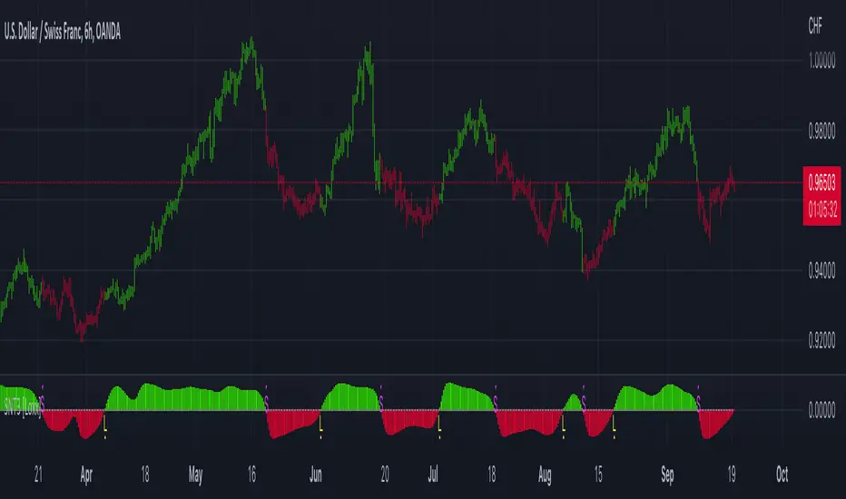
Step Generalized Double DEMA (ATR based) [Loxx]Step Generalized Double DEMA (ATR based) works like a T3 moving average but is less smooth. This is on purpose to catch more signals. The addition of ATR stepped filtering reduces noise while maintaining signal integrity. This one comes via Mr. Tools.
Theory:
The double exponential moving average (DEMA), was developed by Patrick Mulloy in an attempt to reduce the amount of lag time found in traditional moving averages. It was first introduced in the February 1994 issue of the magazine Technical Analysis of Stocks & Commodities in Mulloy's article "Smoothing Data with Faster Moving Averages". The way to calculate is the following :
The Double Exponential Moving Average calculations are based combinations of a single EMA and double EMA into a new EMA:
1. Calculate EMA
2. Calculate Smoothed EMA by applying EMA with the same period to the EMA calculated in the first step
3. Calculate DEMA
DEMA = (2 * EMA) - (Smoothed EMA)
This version:
For our purposes here, we are using Tim Tillson's (the inventor of T3) work, specifically, we are using the GDEMA of GDEMA for calculation (which is the "middle step" of T3 calculation). Since there are no versions showing that "middle step, this version covers that too. The result is smoother than Generalized DEMA, but is less smooth than T3 - one has to do some experimenting in order to find the optimal way to use it, but in any case, since it is "faster" than the T3 (Tim Tillson T3) and still smooth, it looks like a good compromise between speed and smoothness.
Usage:
You can use it as any regular average or you can use the color change of the indicator as a signal.
Included
Alerts
Signals
Bar coloring
Loxx's Expanded Source Types
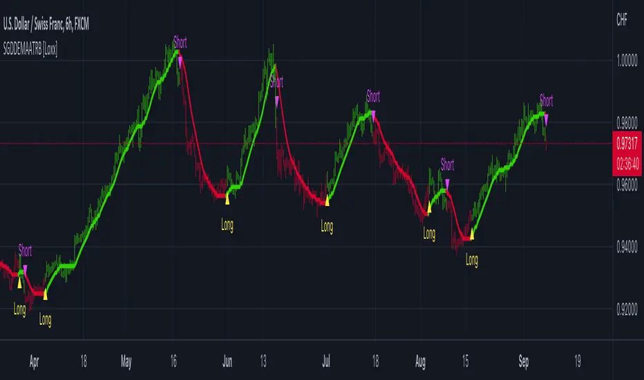
Variety N-Tuple Moving Averages [Loxx]Variety N-Tuple Moving Averages is a moving average indicator that allows you to create 1- 30 tuple moving average types; i.e., Double-MA, Triple-MA, Quadruple-MA, Quintuple-MA, ... N-tuple-MA. This version contains 5 different moving average types including T3. A list of tuples can be found here if you'd like to name the order of the moving average by depth: Tuples extrapolated
You'll notice that this is a lot of code and could normally be packed into a single loop in order to extract the N-tuple MA, however due to Pine Script limitations and processing paradigm this is not possible ... yet.
If you choose the EMA option and select a depth of 2, this is the classic DEMA; EMA with a depth of 3 is the classic TEMA, and so on and so forth this is to help you understand how this indicator works. This version of NTMA is restricted to a maximum depth of 30 or less. Normally this indicator would include 50 depths but I've cut this down to 30 to reduce indicator load time. In the future, I'll create an updated NTMA that allows for more depth levels.
This is considered one of the top ten indicators in forex. You can read more about it here: forex-station.com
How this works
Step 1: Run factorial calculation on the depth value,
Step 2: Calculate weights of nested moving averages
factorial(nemadepth) / (factorial(nemadepth - k) * factorial(k); where nemadepth is the depth and k is the weight position
Examples of coefficient outputs:
6 Depth: 6 15 20 15 6
7 Depth: 7 21 35 35 21 7
8 Depth: 8 28 56 70 56 28 8
9 Depth: 9 36 34 84 126 126 84 36 9
10 Depth: 10 45 120 210 252 210 120 45 10
11 Depth: 11 55 165 330 462 462 330 165 55 11
12 Depth: 12 66 220 495 792 924 792 495 220 66 12
13 Depth: 13 78 286 715 1287 1716 1716 1287 715 286 78 13
Step 3: Apply coefficient to each moving average
For QEMA, which is 5 depth EMA, the caculation is as follows
ema1 = ta.ema(src, length)
ema2 = ta.ema(ema1, length)
ema3 = ta.ema(ema2, length)
ema4 = ta.ema(ema3, length)
ema5 = ta.ema(ema4, length)
qema = 5 * ema1 - 10 * ema2 + 10 * ema3 - 5 * ema4 + ema5
Included:
Alerts
Loxx's Expanded Source Types
Bar coloring
T3 Velocity Candles [Loxx]T3 Velocity Candles is a candle coloring overlay that calculates its gradient coloring using T3 velocity.
What is the T3 moving average?
Better Moving Averages Tim Tillson
November 1, 1998
Tim Tillson is a software project manager at Hewlett-Packard, with degrees in Mathematics and Computer Science. He has privately traded options and equities for 15 years.
Introduction
"Digital filtering includes the process of smoothing, predicting, differentiating, integrating, separation of signals, and removal of noise from a signal. Thus many people who do such things are actually using digital filters without realizing that they are; being unacquainted with the theory, they neither understand what they have done nor the possibilities of what they might have done."
This quote from R. W. Hamming applies to the vast majority of indicators in technical analysis . Moving averages, be they simple, weighted, or exponential, are lowpass filters; low frequency components in the signal pass through with little attenuation, while high frequencies are severely reduced.
"Oscillator" type indicators (such as MACD , Momentum, Relative Strength Index ) are another type of digital filter called a differentiator.
Tushar Chande has observed that many popular oscillators are highly correlated, which is sensible because they are trying to measure the rate of change of the underlying time series, i.e., are trying to be the first and second derivatives we all learned about in Calculus.
We use moving averages (lowpass filters) in technical analysis to remove the random noise from a time series, to discern the underlying trend or to determine prices at which we will take action. A perfect moving average would have two attributes:
It would be smooth, not sensitive to random noise in the underlying time series. Another way of saying this is that its derivative would not spuriously alternate between positive and negative values.
It would not lag behind the time series it is computed from. Lag, of course, produces late buy or sell signals that kill profits.
The only way one can compute a perfect moving average is to have knowledge of the future, and if we had that, we would buy one lottery ticket a week rather than trade!
Having said this, we can still improve on the conventional simple, weighted, or exponential moving averages. Here's how:
Two Interesting Moving Averages
We will examine two benchmark moving averages based on Linear Regression analysis.
In both cases, a Linear Regression line of length n is fitted to price data.
I call the first moving average ILRS, which stands for Integral of Linear Regression Slope. One simply integrates the slope of a linear regression line as it is successively fitted in a moving window of length n across the data, with the constant of integration being a simple moving average of the first n points. Put another way, the derivative of ILRS is the linear regression slope. Note that ILRS is not the same as a SMA ( simple moving average ) of length n, which is actually the midpoint of the linear regression line as it moves across the data.
We can measure the lag of moving averages with respect to a linear trend by computing how they behave when the input is a line with unit slope. Both SMA (n) and ILRS(n) have lag of n/2, but ILRS is much smoother than SMA .
Our second benchmark moving average is well known, called EPMA or End Point Moving Average. It is the endpoint of the linear regression line of length n as it is fitted across the data. EPMA hugs the data more closely than a simple or exponential moving average of the same length. The price we pay for this is that it is much noisier (less smooth) than ILRS, and it also has the annoying property that it overshoots the data when linear trends are present.
However, EPMA has a lag of 0 with respect to linear input! This makes sense because a linear regression line will fit linear input perfectly, and the endpoint of the LR line will be on the input line.
These two moving averages frame the tradeoffs that we are facing. On one extreme we have ILRS, which is very smooth and has considerable phase lag. EPMA has 0 phase lag, but is too noisy and overshoots. We would like to construct a better moving average which is as smooth as ILRS, but runs closer to where EPMA lies, without the overshoot.
A easy way to attempt this is to split the difference, i.e. use (ILRS(n)+EPMA(n))/2. This will give us a moving average (call it IE /2) which runs in between the two, has phase lag of n/4 but still inherits considerable noise from EPMA. IE /2 is inspirational, however. Can we build something that is comparable, but smoother? Figure 1 shows ILRS, EPMA, and IE /2.
Filter Techniques
Any thoughtful student of filter theory (or resolute experimenter) will have noticed that you can improve the smoothness of a filter by running it through itself multiple times, at the cost of increasing phase lag.
There is a complementary technique (called twicing by J.W. Tukey) which can be used to improve phase lag. If L stands for the operation of running data through a low pass filter, then twicing can be described by:
L' = L(time series) + L(time series - L(time series))
That is, we add a moving average of the difference between the input and the moving average to the moving average. This is algebraically equivalent to:
2L-L(L)
This is the Double Exponential Moving Average or DEMA , popularized by Patrick Mulloy in TASAC (January/February 1994).
In our taxonomy, DEMA has some phase lag (although it exponentially approaches 0) and is somewhat noisy, comparable to IE /2 indicator.
We will use these two techniques to construct our better moving average, after we explore the first one a little more closely.
Fixing Overshoot
An n-day EMA has smoothing constant alpha=2/(n+1) and a lag of (n-1)/2.
Thus EMA (3) has lag 1, and EMA (11) has lag 5. Figure 2 shows that, if I am willing to incur 5 days of lag, I get a smoother moving average if I run EMA (3) through itself 5 times than if I just take EMA (11) once.
This suggests that if EPMA and DEMA have 0 or low lag, why not run fast versions (eg DEMA (3)) through themselves many times to achieve a smooth result? The problem is that multiple runs though these filters increase their tendency to overshoot the data, giving an unusable result. This is because the amplitude response of DEMA and EPMA is greater than 1 at certain frequencies, giving a gain of much greater than 1 at these frequencies when run though themselves multiple times. Figure 3 shows DEMA (7) and EPMA(7) run through themselves 3 times. DEMA^3 has serious overshoot, and EPMA^3 is terrible.
The solution to the overshoot problem is to recall what we are doing with twicing:
DEMA (n) = EMA (n) + EMA (time series - EMA (n))
The second term is adding, in effect, a smooth version of the derivative to the EMA to achieve DEMA . The derivative term determines how hot the moving average's response to linear trends will be. We need to simply turn down the volume to achieve our basic building block:
EMA (n) + EMA (time series - EMA (n))*.7;
This is algebraically the same as:
EMA (n)*1.7-EMA( EMA (n))*.7;
I have chosen .7 as my volume factor, but the general formula (which I call "Generalized Dema") is:
GD (n,v) = EMA (n)*(1+v)-EMA( EMA (n))*v,
Where v ranges between 0 and 1. When v=0, GD is just an EMA , and when v=1, GD is DEMA . In between, GD is a cooler DEMA . By using a value for v less than 1 (I like .7), we cure the multiple DEMA overshoot problem, at the cost of accepting some additional phase delay. Now we can run GD through itself multiple times to define a new, smoother moving average T3 that does not overshoot the data:
T3(n) = GD ( GD ( GD (n)))
In filter theory parlance, T3 is a six-pole non-linear Kalman filter. Kalman filters are ones which use the error (in this case (time series - EMA (n)) to correct themselves. In Technical Analysis , these are called Adaptive Moving Averages; they track the time series more aggressively when it is making large moves.

T3 Striped [Loxx]Theory:
Although T3 is widely used, some of the details on how it is calculated are less known. T3 has, internally, 6 "levels" or "steps" that it uses for its calculation.
This version:
Instead of showing the final T3 value, this indicator shows those intermediate steps. This shows the "building steps" of T3 and can be used for trend assessment as well as for possible support / resistance values.
What is the T3 moving average?
Better Moving Averages Tim Tillson
November 1, 1998
Tim Tillson is a software project manager at Hewlett-Packard, with degrees in Mathematics and Computer Science. He has privately traded options and equities for 15 years.
Introduction
"Digital filtering includes the process of smoothing, predicting, differentiating, integrating, separation of signals, and removal of noise from a signal. Thus many people who do such things are actually using digital filters without realizing that they are; being unacquainted with the theory, they neither understand what they have done nor the possibilities of what they might have done."
This quote from R. W. Hamming applies to the vast majority of indicators in technical analysis . Moving averages, be they simple, weighted, or exponential, are lowpass filters; low frequency components in the signal pass through with little attenuation, while high frequencies are severely reduced.
"Oscillator" type indicators (such as MACD , Momentum, Relative Strength Index ) are another type of digital filter called a differentiator.
Tushar Chande has observed that many popular oscillators are highly correlated, which is sensible because they are trying to measure the rate of change of the underlying time series, i.e., are trying to be the first and second derivatives we all learned about in Calculus.
We use moving averages (lowpass filters) in technical analysis to remove the random noise from a time series, to discern the underlying trend or to determine prices at which we will take action. A perfect moving average would have two attributes:
It would be smooth, not sensitive to random noise in the underlying time series. Another way of saying this is that its derivative would not spuriously alternate between positive and negative values.
It would not lag behind the time series it is computed from. Lag, of course, produces late buy or sell signals that kill profits.
The only way one can compute a perfect moving average is to have knowledge of the future, and if we had that, we would buy one lottery ticket a week rather than trade!
Having said this, we can still improve on the conventional simple, weighted, or exponential moving averages. Here's how:
Two Interesting Moving Averages
We will examine two benchmark moving averages based on Linear Regression analysis.
In both cases, a Linear Regression line of length n is fitted to price data.
I call the first moving average ILRS, which stands for Integral of Linear Regression Slope. One simply integrates the slope of a linear regression line as it is successively fitted in a moving window of length n across the data, with the constant of integration being a simple moving average of the first n points. Put another way, the derivative of ILRS is the linear regression slope. Note that ILRS is not the same as a SMA ( simple moving average ) of length n, which is actually the midpoint of the linear regression line as it moves across the data.
We can measure the lag of moving averages with respect to a linear trend by computing how they behave when the input is a line with unit slope. Both SMA (n) and ILRS(n) have lag of n/2, but ILRS is much smoother than SMA .
Our second benchmark moving average is well known, called EPMA or End Point Moving Average. It is the endpoint of the linear regression line of length n as it is fitted across the data. EPMA hugs the data more closely than a simple or exponential moving average of the same length. The price we pay for this is that it is much noisier (less smooth) than ILRS, and it also has the annoying property that it overshoots the data when linear trends are present.
However, EPMA has a lag of 0 with respect to linear input! This makes sense because a linear regression line will fit linear input perfectly, and the endpoint of the LR line will be on the input line.
These two moving averages frame the tradeoffs that we are facing. On one extreme we have ILRS, which is very smooth and has considerable phase lag. EPMA has 0 phase lag, but is too noisy and overshoots. We would like to construct a better moving average which is as smooth as ILRS, but runs closer to where EPMA lies, without the overshoot.
A easy way to attempt this is to split the difference, i.e. use (ILRS(n)+EPMA(n))/2. This will give us a moving average (call it IE /2) which runs in between the two, has phase lag of n/4 but still inherits considerable noise from EPMA. IE /2 is inspirational, however. Can we build something that is comparable, but smoother? Figure 1 shows ILRS, EPMA, and IE /2.
Filter Techniques
Any thoughtful student of filter theory (or resolute experimenter) will have noticed that you can improve the smoothness of a filter by running it through itself multiple times, at the cost of increasing phase lag.
There is a complementary technique (called twicing by J.W. Tukey) which can be used to improve phase lag. If L stands for the operation of running data through a low pass filter, then twicing can be described by:
L' = L(time series) + L(time series - L(time series))
That is, we add a moving average of the difference between the input and the moving average to the moving average. This is algebraically equivalent to:
2L-L(L)
This is the Double Exponential Moving Average or DEMA , popularized by Patrick Mulloy in TASAC (January/February 1994).
In our taxonomy, DEMA has some phase lag (although it exponentially approaches 0) and is somewhat noisy, comparable to IE /2 indicator.
We will use these two techniques to construct our better moving average, after we explore the first one a little more closely.
Fixing Overshoot
An n-day EMA has smoothing constant alpha=2/(n+1) and a lag of (n-1)/2.
Thus EMA (3) has lag 1, and EMA (11) has lag 5. Figure 2 shows that, if I am willing to incur 5 days of lag, I get a smoother moving average if I run EMA (3) through itself 5 times than if I just take EMA (11) once.
This suggests that if EPMA and DEMA have 0 or low lag, why not run fast versions (eg DEMA (3)) through themselves many times to achieve a smooth result? The problem is that multiple runs though these filters increase their tendency to overshoot the data, giving an unusable result. This is because the amplitude response of DEMA and EPMA is greater than 1 at certain frequencies, giving a gain of much greater than 1 at these frequencies when run though themselves multiple times. Figure 3 shows DEMA (7) and EPMA(7) run through themselves 3 times. DEMA^3 has serious overshoot, and EPMA^3 is terrible.
The solution to the overshoot problem is to recall what we are doing with twicing:
DEMA (n) = EMA (n) + EMA (time series - EMA (n))
The second term is adding, in effect, a smooth version of the derivative to the EMA to achieve DEMA . The derivative term determines how hot the moving average's response to linear trends will be. We need to simply turn down the volume to achieve our basic building block:
EMA (n) + EMA (time series - EMA (n))*.7;
This is algebraically the same as:
EMA (n)*1.7-EMA( EMA (n))*.7;
I have chosen .7 as my volume factor, but the general formula (which I call "Generalized Dema") is:
GD (n,v) = EMA (n)*(1+v)-EMA( EMA (n))*v,
Where v ranges between 0 and 1. When v=0, GD is just an EMA , and when v=1, GD is DEMA . In between, GD is a cooler DEMA . By using a value for v less than 1 (I like .7), we cure the multiple DEMA overshoot problem, at the cost of accepting some additional phase delay. Now we can run GD through itself multiple times to define a new, smoother moving average T3 that does not overshoot the data:
T3(n) = GD ( GD ( GD (n)))
In filter theory parlance, T3 is a six-pole non-linear Kalman filter. Kalman filters are ones which use the error (in this case (time series - EMA (n)) to correct themselves. In Technical Analysis , these are called Adaptive Moving Averages; they track the time series more aggressively when it is making large moves.
Included
Alerts
Signals
Bar coloring
Loxx's Expanded Source Types
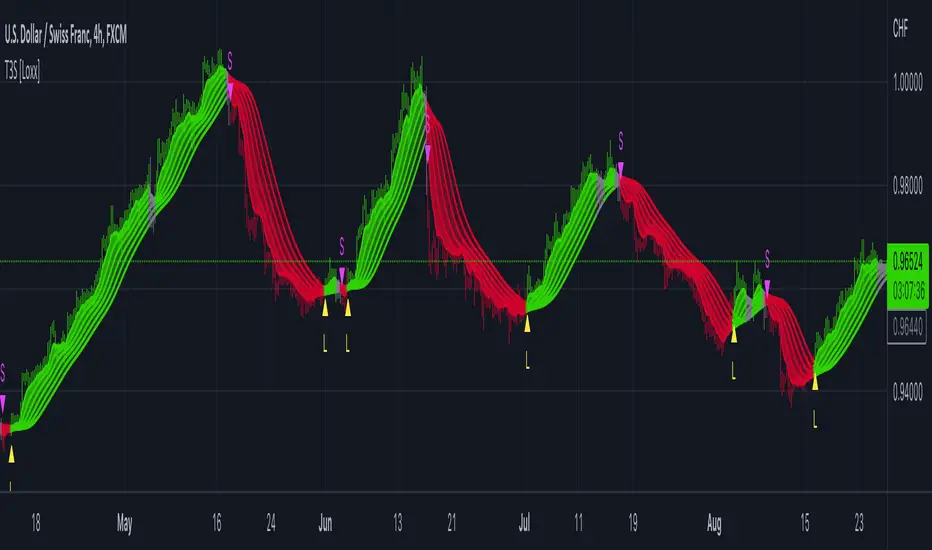
R-squared Adaptive T3 Ribbon Filled Simple [Loxx]R-squared Adaptive T3 Ribbon Filled Simple is a T3 ribbons indicator that uses a special implementation of T3 that is R-squared adaptive.
What is the T3 moving average?
Better Moving Averages Tim Tillson
November 1, 1998
Tim Tillson is a software project manager at Hewlett-Packard, with degrees in Mathematics and Computer Science. He has privately traded options and equities for 15 years.
Introduction
"Digital filtering includes the process of smoothing, predicting, differentiating, integrating, separation of signals, and removal of noise from a signal. Thus many people who do such things are actually using digital filters without realizing that they are; being unacquainted with the theory, they neither understand what they have done nor the possibilities of what they might have done."
This quote from R. W. Hamming applies to the vast majority of indicators in technical analysis . Moving averages, be they simple, weighted, or exponential, are lowpass filters; low frequency components in the signal pass through with little attenuation, while high frequencies are severely reduced.
"Oscillator" type indicators (such as MACD , Momentum, Relative Strength Index ) are another type of digital filter called a differentiator.
Tushar Chande has observed that many popular oscillators are highly correlated, which is sensible because they are trying to measure the rate of change of the underlying time series, i.e., are trying to be the first and second derivatives we all learned about in Calculus.
We use moving averages (lowpass filters) in technical analysis to remove the random noise from a time series, to discern the underlying trend or to determine prices at which we will take action. A perfect moving average would have two attributes:
It would be smooth, not sensitive to random noise in the underlying time series. Another way of saying this is that its derivative would not spuriously alternate between positive and negative values.
It would not lag behind the time series it is computed from. Lag, of course, produces late buy or sell signals that kill profits.
The only way one can compute a perfect moving average is to have knowledge of the future, and if we had that, we would buy one lottery ticket a week rather than trade!
Having said this, we can still improve on the conventional simple, weighted, or exponential moving averages. Here's how:
Two Interesting Moving Averages
We will examine two benchmark moving averages based on Linear Regression analysis.
In both cases, a Linear Regression line of length n is fitted to price data.
I call the first moving average ILRS, which stands for Integral of Linear Regression Slope. One simply integrates the slope of a linear regression line as it is successively fitted in a moving window of length n across the data, with the constant of integration being a simple moving average of the first n points. Put another way, the derivative of ILRS is the linear regression slope. Note that ILRS is not the same as a SMA ( simple moving average ) of length n, which is actually the midpoint of the linear regression line as it moves across the data.
We can measure the lag of moving averages with respect to a linear trend by computing how they behave when the input is a line with unit slope. Both SMA (n) and ILRS(n) have lag of n/2, but ILRS is much smoother than SMA .
Our second benchmark moving average is well known, called EPMA or End Point Moving Average. It is the endpoint of the linear regression line of length n as it is fitted across the data. EPMA hugs the data more closely than a simple or exponential moving average of the same length. The price we pay for this is that it is much noisier (less smooth) than ILRS, and it also has the annoying property that it overshoots the data when linear trends are present.
However, EPMA has a lag of 0 with respect to linear input! This makes sense because a linear regression line will fit linear input perfectly, and the endpoint of the LR line will be on the input line.
These two moving averages frame the tradeoffs that we are facing. On one extreme we have ILRS, which is very smooth and has considerable phase lag. EPMA has 0 phase lag, but is too noisy and overshoots. We would like to construct a better moving average which is as smooth as ILRS, but runs closer to where EPMA lies, without the overshoot.
A easy way to attempt this is to split the difference, i.e. use (ILRS(n)+EPMA(n))/2. This will give us a moving average (call it IE /2) which runs in between the two, has phase lag of n/4 but still inherits considerable noise from EPMA. IE /2 is inspirational, however. Can we build something that is comparable, but smoother? Figure 1 shows ILRS, EPMA, and IE /2.
Filter Techniques
Any thoughtful student of filter theory (or resolute experimenter) will have noticed that you can improve the smoothness of a filter by running it through itself multiple times, at the cost of increasing phase lag.
There is a complementary technique (called twicing by J.W. Tukey) which can be used to improve phase lag. If L stands for the operation of running data through a low pass filter, then twicing can be described by:
L' = L(time series) + L(time series - L(time series))
That is, we add a moving average of the difference between the input and the moving average to the moving average. This is algebraically equivalent to:
2L-L(L)
This is the Double Exponential Moving Average or DEMA , popularized by Patrick Mulloy in TASAC (January/February 1994).
In our taxonomy, DEMA has some phase lag (although it exponentially approaches 0) and is somewhat noisy, comparable to IE /2 indicator.
We will use these two techniques to construct our better moving average, after we explore the first one a little more closely.
Fixing Overshoot
An n-day EMA has smoothing constant alpha=2/(n+1) and a lag of (n-1)/2.
Thus EMA (3) has lag 1, and EMA (11) has lag 5. Figure 2 shows that, if I am willing to incur 5 days of lag, I get a smoother moving average if I run EMA (3) through itself 5 times than if I just take EMA (11) once.
This suggests that if EPMA and DEMA have 0 or low lag, why not run fast versions (eg DEMA (3)) through themselves many times to achieve a smooth result? The problem is that multiple runs though these filters increase their tendency to overshoot the data, giving an unusable result. This is because the amplitude response of DEMA and EPMA is greater than 1 at certain frequencies, giving a gain of much greater than 1 at these frequencies when run though themselves multiple times. Figure 3 shows DEMA (7) and EPMA(7) run through themselves 3 times. DEMA^3 has serious overshoot, and EPMA^3 is terrible.
The solution to the overshoot problem is to recall what we are doing with twicing:
DEMA (n) = EMA (n) + EMA (time series - EMA (n))
The second term is adding, in effect, a smooth version of the derivative to the EMA to achieve DEMA . The derivative term determines how hot the moving average's response to linear trends will be. We need to simply turn down the volume to achieve our basic building block:
EMA (n) + EMA (time series - EMA (n))*.7;
This is algebraically the same as:
EMA (n)*1.7-EMA( EMA (n))*.7;
I have chosen .7 as my volume factor, but the general formula (which I call "Generalized Dema") is:
GD (n,v) = EMA (n)*(1+v)-EMA( EMA (n))*v,
Where v ranges between 0 and 1. When v=0, GD is just an EMA , and when v=1, GD is DEMA . In between, GD is a cooler DEMA . By using a value for v less than 1 (I like .7), we cure the multiple DEMA overshoot problem, at the cost of accepting some additional phase delay. Now we can run GD through itself multiple times to define a new, smoother moving average T3 that does not overshoot the data:
T3(n) = GD ( GD ( GD (n)))
In filter theory parlance, T3 is a six-pole non-linear Kalman filter. Kalman filters are ones which use the error (in this case (time series - EMA (n)) to correct themselves. In Technical Analysis , these are called Adaptive Moving Averages; they track the time series more aggressively when it is making large moves.
What is R-squared Adaptive?
One tool available in forecasting the trendiness of the breakout is the coefficient of determination ( R-squared ), a statistical measurement.
The R-squared indicates linear strength between the security's price (the Y - axis) and time (the X - axis). The R-squared is the percentage of squared error that the linear regression can eliminate if it were used as the predictor instead of the mean value. If the R-squared were 0.99, then the linear regression would eliminate 99% of the error for prediction versus predicting closing prices using a simple moving average .
R-squared is used here to derive a T3 factor used to modify price before passing price through a six-pole non-linear Kalman filter.
Included:
Alerts
Signals
Loxx's Expanded Source Types
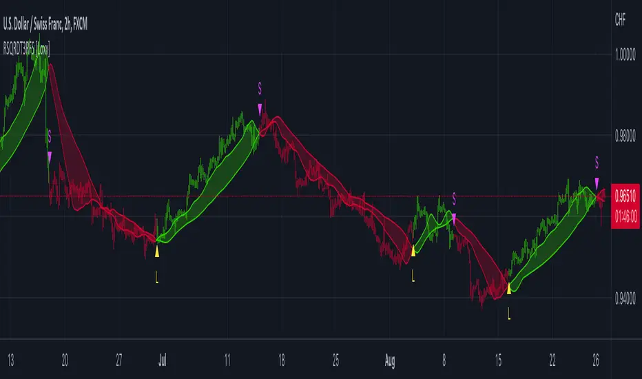
T3 Slope Variation [Loxx]T3 Slope Variation is an indicator that uses T3 moving average to calculate a slope that is then weighted to derive a signal.
The center line
The center line changes color depending on the value of the:
Slope
Signal line
Threshold
If the value is above a signal line (it is not visible on the chart) and the threshold is greater than the required, then the main trend becomes up. And reversed for the trend down.
Colors and style of the histogram
The colors and style of the histogram will be drawn if the value is at the right side, if the above described trend "agrees" with the value (above is green or below zero is red) and if the High is higher than the previous High or Low is lower than the previous low, then the according type of histogram is drawn.
What is the T3 moving average?
Better Moving Averages Tim Tillson
November 1, 1998
Tim Tillson is a software project manager at Hewlett-Packard, with degrees in Mathematics and Computer Science. He has privately traded options and equities for 15 years.
Introduction
"Digital filtering includes the process of smoothing, predicting, differentiating, integrating, separation of signals, and removal of noise from a signal. Thus many people who do such things are actually using digital filters without realizing that they are; being unacquainted with the theory, they neither understand what they have done nor the possibilities of what they might have done."
This quote from R. W. Hamming applies to the vast majority of indicators in technical analysis . Moving averages, be they simple, weighted, or exponential, are lowpass filters; low frequency components in the signal pass through with little attenuation, while high frequencies are severely reduced.
"Oscillator" type indicators (such as MACD , Momentum, Relative Strength Index ) are another type of digital filter called a differentiator.
Tushar Chande has observed that many popular oscillators are highly correlated, which is sensible because they are trying to measure the rate of change of the underlying time series, i.e., are trying to be the first and second derivatives we all learned about in Calculus.
We use moving averages (lowpass filters) in technical analysis to remove the random noise from a time series, to discern the underlying trend or to determine prices at which we will take action. A perfect moving average would have two attributes:
It would be smooth, not sensitive to random noise in the underlying time series. Another way of saying this is that its derivative would not spuriously alternate between positive and negative values.
It would not lag behind the time series it is computed from. Lag, of course, produces late buy or sell signals that kill profits.
The only way one can compute a perfect moving average is to have knowledge of the future, and if we had that, we would buy one lottery ticket a week rather than trade!
Having said this, we can still improve on the conventional simple, weighted, or exponential moving averages. Here's how:
Two Interesting Moving Averages
We will examine two benchmark moving averages based on Linear Regression analysis.
In both cases, a Linear Regression line of length n is fitted to price data.
I call the first moving average ILRS, which stands for Integral of Linear Regression Slope. One simply integrates the slope of a linear regression line as it is successively fitted in a moving window of length n across the data, with the constant of integration being a simple moving average of the first n points. Put another way, the derivative of ILRS is the linear regression slope. Note that ILRS is not the same as a SMA ( simple moving average ) of length n, which is actually the midpoint of the linear regression line as it moves across the data.
We can measure the lag of moving averages with respect to a linear trend by computing how they behave when the input is a line with unit slope. Both SMA (n) and ILRS(n) have lag of n/2, but ILRS is much smoother than SMA .
Our second benchmark moving average is well known, called EPMA or End Point Moving Average. It is the endpoint of the linear regression line of length n as it is fitted across the data. EPMA hugs the data more closely than a simple or exponential moving average of the same length. The price we pay for this is that it is much noisier (less smooth) than ILRS, and it also has the annoying property that it overshoots the data when linear trends are present.
However, EPMA has a lag of 0 with respect to linear input! This makes sense because a linear regression line will fit linear input perfectly, and the endpoint of the LR line will be on the input line.
These two moving averages frame the tradeoffs that we are facing. On one extreme we have ILRS, which is very smooth and has considerable phase lag. EPMA has 0 phase lag, but is too noisy and overshoots. We would like to construct a better moving average which is as smooth as ILRS, but runs closer to where EPMA lies, without the overshoot.
A easy way to attempt this is to split the difference, i.e. use (ILRS(n)+EPMA(n))/2. This will give us a moving average (call it IE /2) which runs in between the two, has phase lag of n/4 but still inherits considerable noise from EPMA. IE /2 is inspirational, however. Can we build something that is comparable, but smoother? Figure 1 shows ILRS, EPMA, and IE /2.
Filter Techniques
Any thoughtful student of filter theory (or resolute experimenter) will have noticed that you can improve the smoothness of a filter by running it through itself multiple times, at the cost of increasing phase lag.
There is a complementary technique (called twicing by J.W. Tukey) which can be used to improve phase lag. If L stands for the operation of running data through a low pass filter, then twicing can be described by:
L' = L(time series) + L(time series - L(time series))
That is, we add a moving average of the difference between the input and the moving average to the moving average. This is algebraically equivalent to:
2L-L(L)
This is the Double Exponential Moving Average or DEMA , popularized by Patrick Mulloy in TASAC (January/February 1994).
In our taxonomy, DEMA has some phase lag (although it exponentially approaches 0) and is somewhat noisy, comparable to IE /2 indicator.
We will use these two techniques to construct our better moving average, after we explore the first one a little more closely.
Fixing Overshoot
An n-day EMA has smoothing constant alpha=2/(n+1) and a lag of (n-1)/2.
Thus EMA (3) has lag 1, and EMA (11) has lag 5. Figure 2 shows that, if I am willing to incur 5 days of lag, I get a smoother moving average if I run EMA (3) through itself 5 times than if I just take EMA (11) once.
This suggests that if EPMA and DEMA have 0 or low lag, why not run fast versions (eg DEMA (3)) through themselves many times to achieve a smooth result? The problem is that multiple runs though these filters increase their tendency to overshoot the data, giving an unusable result. This is because the amplitude response of DEMA and EPMA is greater than 1 at certain frequencies, giving a gain of much greater than 1 at these frequencies when run though themselves multiple times. Figure 3 shows DEMA (7) and EPMA(7) run through themselves 3 times. DEMA^3 has serious overshoot, and EPMA^3 is terrible.
The solution to the overshoot problem is to recall what we are doing with twicing:
DEMA (n) = EMA (n) + EMA (time series - EMA (n))
The second term is adding, in effect, a smooth version of the derivative to the EMA to achieve DEMA . The derivative term determines how hot the moving average's response to linear trends will be. We need to simply turn down the volume to achieve our basic building block:
EMA (n) + EMA (time series - EMA (n))*.7;
This is algebraically the same as:
EMA (n)*1.7-EMA( EMA (n))*.7;
I have chosen .7 as my volume factor, but the general formula (which I call "Generalized Dema") is:
GD (n,v) = EMA (n)*(1+v)-EMA( EMA (n))*v,
Where v ranges between 0 and 1. When v=0, GD is just an EMA , and when v=1, GD is DEMA . In between, GD is a cooler DEMA . By using a value for v less than 1 (I like .7), we cure the multiple DEMA overshoot problem, at the cost of accepting some additional phase delay. Now we can run GD through itself multiple times to define a new, smoother moving average T3 that does not overshoot the data:
T3(n) = GD ( GD ( GD (n)))
In filter theory parlance, T3 is a six-pole non-linear Kalman filter. Kalman filters are ones which use the error (in this case (time series - EMA (n)) to correct themselves. In Technical Analysis , these are called Adaptive Moving Averages; they track the time series more aggressively when it is making large moves.
Included
Alets
Signals
Bar coloring
Loxx's Expanded Source Types