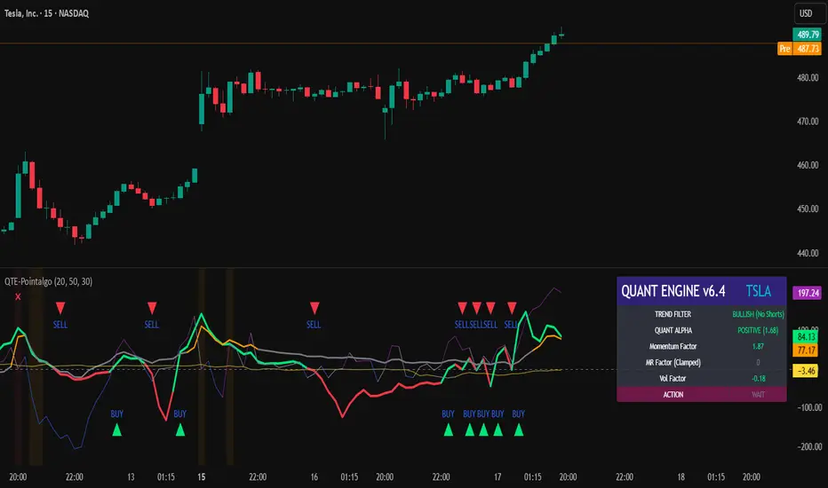
QUANT TRADING ENGINE [PointAlgo]Quant Trading Engine is a quantitative market-analysis indicator that combines multiple statistical factors to study trend behavior, mean reversion, volatility, execution efficiency, and market stability.
The indicator converts raw price behavior into standardized signals to help evaluate directional bias and risk conditions in a systematic way.
This script focuses on factor alignment and regime awareness, not prediction certainty.
Design Philosophy
Markets move through different regimes such as trending, ranging, volatile expansion, and instability.
This indicator attempts to model these regimes by blending:
Momentum strength
Mean-reversion pressure
Volatility risk
Trend filtering
Execution context (VWAP)
Correlation structure
Each component is normalized and combined into a single Quant Alpha framework.
Factor Construction
1. Momentum Factor
Measures directional strength using percentage price change over a rolling window.
Standardized using mean and standard deviation.
Represents trend continuation pressure.
2. Mean Reversion Factor
Measures deviation from a longer moving average.
Standardized to identify stretched conditions.
Designed to capture counter-trend behavior.
Directional Clamping
Mean-reversion signals are dynamically restricted:
No counter-trend buying during downtrends.
No counter-trend selling during uptrends.
Allows both sides only in neutral regimes.
This prevents conflicting signals in strong trends.
3. Volatility Factor
Uses realized volatility derived from price changes.
Penalizes environments where volatility deviates significantly from its norm.
Acts as a risk adjustment rather than a directional driver.
4. Composite Quant Alpha
The final Quant Alpha is a weighted blend of:
Momentum
Mean reversion (trend-clamped)
Volatility risk
The composite is standardized into a Z-score, allowing consistent interpretation across instruments and timeframes.
Signal Logic
Buy signal occurs when Quant Alpha crosses above zero.
Sell signal occurs when Quant Alpha crosses below zero.
Zero-cross logic is used to represent shifts from negative to positive statistical bias and vice versa.
Signals reflect statistical regime change, not trade instructions.
Volatility Smile Context
Measures price deviation from its statistical distribution.
Identifies skewed conditions where upside or downside volatility becomes dominant.
Highlights extreme deviations that may imply elevated derivative risk.
Exotic Risk Conditions
Detects sudden price expansion combined with volatility spikes.
Highlights environments where execution and risk become unstable.
Visual background cues are used for awareness only.
Execution Context (VWAP)
Measures price distance from VWAP.
Used to assess execution efficiency rather than direction.
Helps identify stretched conditions relative to average traded price.
Correlation Structure
Evaluates short-term return correlations.
Detects when price behavior becomes less predictable.
Flags structural instability rather than trend direction.
Visualization
The indicator plots:
Quant Alpha (scaled) with directional coloring
Volatility smile deviation
Price vs VWAP distance
Correlation structure
Signal markers indicate Quant Alpha zero-cross events and risk conditions.
Dashboard
A compact dashboard summarizes:
Trend filter state
Quant Alpha polarity and value
Individual factor readings
Current action state (Buy / Sell / Wait / Risk)
The dashboard provides a real-time snapshot of internal model conditions.
Usage Notes
Designed for analytical interpretation and research.
Best used alongside price action and risk management tools.
Factor behavior depends on instrument liquidity and volatility.
Not optimized for illiquid or irregular markets.
Disclaimer
This script is provided for educational and analytical purposes only.
It does not provide financial, investment, or trading advice.
All outputs should be independently validated before making any trading decisions.
Algotrading
Ace Algo [Anson5129]🏆 Exclusive Indicator: Ace Algo
📈 Works for stocks, forex, crypto, indices
📈 Easy to use, real-time alerts, no repaint
📈 No grid, no martingale, no hedging
📈 One position at a time
----------------------------------------------------------------------------------------
Ace Algo
A trend-following TradingView strategy using a confluence of technical indicators and time-based rules for structured long/short entries and exits:
----------------------------------------------------------------------------------------
Parameters Explanation
Moving Average Length
Indicates the number of historical data points used for the average price calculation.
Shorter = volatile (short-term trends); longer = smoother (long-term trends, less noise).
Default: 20
Entry delay in bars
After a trade is closed, delay the next entry in bars. The lower the number, the more trades you will get.
Default: 4
Take Profit delay in bars
After a trade is opened, delay the take profit in bars. The lower the number, the more trades you will get.
Default: 3
Enable ADX Filter
No order will be placed when ADX < 20
Default: Uncheck
Block Period
Set a block period during which no trading will take place.
----------------------------------------------------------------------------------------
Entry Condition:
Only Long when the price is above the moving average (Orange line).
Only Short when the price is below the moving average (Orange line).
* Also, with some hidden parameter that I set in the backend.
Exit Condition:
When getting profit:
Trailing Stop Activates after a position has been open for a set number of bars (to avoid premature exits).
When losing money:
In a long position, when the price falls below the moving average, and the conditions for a short position are met, the long position will be closed, and the short position will be opened.
In a short position, when the price rises above the moving average, and the conditions for a long position are met, the short position will be closed, and the long position will be opened.
----------------------------------------------------------------------------------------
How to get access to the strategy
Read the author's instructions on the right to learn how to get access to the strategy.

Vega Convexity Engine [PRO]ENGINEERED ASYMMETRY.
This is the flagship Stage 2 Specialist Model of the Vega Crypto Strategies ecosystem.
While the free "Regime Filter" tells you when to trade (filtering out chop), the Convexity Engine tells you how to trade. It activates only when the Regime Filter confirms an Impulse, classifying the specific vector of the market move to maximize risk-adjusted returns.
PRO FEATURES
This script visualizes the output of our Hierarchical Machine Learning Engine:
🚀 Directional Classification:
It does not just say "Buy." It classifies volatility into 4 distinct probability classes:
- EXPLOSION: High-confidence, high-velocity upside (Fat-Tail).
- RALLY: Standard trend continuation.
- PULLBACK: Short-term correction opportunity.
- CRASH: High-confidence downside (Long Squeeze Detection).
🛡️ Dynamic Risk Engine (Intraday Stops):
The "+" markers on your chart represent the Vega Institutional Stop Loss . These levels dynamically adjust based on Average True Range (ATR) and Volatility Z-Scores.
Strategy: If price breaches the "+" marker, the hypothesis is invalidated. Exit immediately.
📊 Institutional HUD:
A professional heads-up display showing the current Regime, Vector, and Risk Deployment status in real-time.
THE PHILOSOPHY
"Convexity" means limited downside with unlimited upside. By combining the Regime Filter (sitting in cash during noise) with Dynamic Stops (cutting losers fast), this engine is designed to capture the "fat tails" of the crypto market distribution.
🔒 HOW TO GET ACCESS
This is an Invite-Only script. It is strictly for members of Vega Crypto Strategies .
To unlock access, please visit the link in the Author Profile below or check our signature. Once subscribed via Whop, your TradingView username will be automatically authorized instantly.
Disclaimer: This tool is for educational purposes only. Past performance is not indicative of future results. Trading cryptocurrencies involves significant risk.

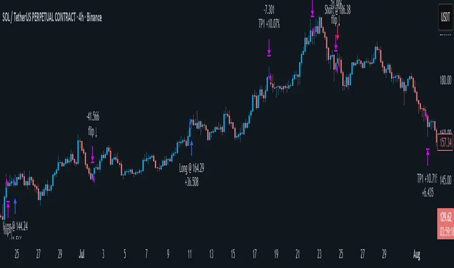
RiskyInvesting Algo v1.0.0 FREEA multi‑layer trend‑following and momentum‑confirmation system designed around dual adaptive baselines, Heikin‑Ashi structure, and smart candle‑strength filtering. This strategy blends volatility‑based trailing logic with macro trend bias tools (EMA + SMMA) to identify clean directional flips and filter out weak signals.
This model uses 5 parameters, while the Pro uses 9 parameters. For more info, follow me on Twitter/X
Disclaimer:
- You must use the Heikin-Ashi candle type for this indicator.
- Please use this in conjunction with your trading system. Labels are not meant to be used as financial advice.
Core features include:
- Heikin‑Ashi Transformation: Smooths price action for more reliable trend identification.
- Two Adaptive Trailing Baselines: ATR‑adjusted equations (Parameter 1 & 2) that flip direction based on baseline breaks.
- Directional Shift Detection: Buy signals on bullish dual‑baseline flip; sell signals on bearish dual‑baseline flip.
- Trend Bias Filtering: Uses EMA vs SMMA relationship to color signals and provide market bias context.
- Candle Strength Filter: Ensures signals only trigger on meaningful momentum candles relative to ATR.
- Clean Visual Display: Auto‑coloring buy/sell labels, baseline plots, and signal triangles.
🟩 = Full Position
🟦 = Half Position
🟥 = Full Position
🟧 = Half Position
Built for traders who want a structured trend‑flip system that avoids noise, highlights strong directional moments, and maintains visual clarity even on volatile intraday charts.

Mutanabby_AI | ONEUSDT_MR1
ONEUSDT Mean-Reversion Strategy | 74.68% Win Rate | 417% Net Profit
This is a long-only mean-reversion strategy designed specifically for ONEUSDT on the 1-hour timeframe. The core logic identifies oversold conditions following sharp declines and enters positions when selling pressure exhausts, capturing the subsequent recovery bounce.
Backtested Period: June 2019 – December 2025 (~6 years)
Performance Summary
| Metric | Value |
|--------|-------|
| Net Profit | +417.68% |
| Win Rate | 74.68% |
| Profit Factor | 4.019 |
| Total Trades | 237 |
| Sharpe Ratio | 0.364 |
| Sortino Ratio | 1.917 |
| Max Drawdown | 51.08% |
| Avg Win | +3.14% |
| Avg Loss | -2.30% |
| Buy & Hold Return | -80.44% |
Strategy Logic :
Entry Conditions (Long Only):
The strategy seeks confluence of three conditions that identify exhausted selling:
1. Prior Move Filter:*The price change from 5 bars ago to 3 bars ago must be ≥ -7% (ensures we're not entering during freefall)
2. Current Move Filter: The price change over the last 2 bars must be ≤ 0% (confirms momentum is stalling or reversing)
3. Three-Bar Decline: The price change from 5 bars ago to 3 bars ago must be ≤ -5% (confirms a significant recent drop occurred)
When all three conditions align, the strategy identifies a potential reversal point where sellers are exhausted.
Exit Conditions:
- Primary Exit: Close above the previous bar's high while the open of the previous bar is at or below the close from 9 bars ago (profit-taking on strength)
- Trailing Stop: 11x ATR trailing stop that locks in profits as price rises
Risk Management
- Position Sizing:Fixed position based on account equity divided by entry price
- Trailing Stop:11× ATR (14-period) provides wide enough room for crypto volatility while protecting gains
- Pyramiding:Up to 4 orders allowed (can scale into winning positions)
- **Commission:** 0.1% per trade (realistic exchange fees included)
Important Disclaimers
⚠️ This is NOT financial advice.
- Past performance does not guarantee future results
- Backtest results may contain look-ahead bias or curve-fitting
- Real trading involves slippage, liquidity issues, and execution delays
- This strategy is optimized for ONEUSDT specifically — results may differ on other pairs
- Always test before risking real capital
Recommended Usage
- Timeframe:*1H (as designed)
- Pair: ONEUSDT (Binance)
- Account Size: Ensure sufficient capital to survive max drawdown
Source Code
Feedback Welcome
I'm sharing this strategy freely for educational purposes. Please:
- Drop a comment with your backtesting results any you analysis
- Share any modifications that improve performance
- Let me know if you spot any issues in the logic
Happy trading
As a quant trader, do you think this strategy will survive in live trading?
Yes or No? And why?
I want to hear from you guys

BaraaCoOL's Multi-Timeframe Signals**BaraaCoOL's RTD - Real-Time Direction Indicator**
© BaraaCoOL 2025 | Version 1.0
**🎯 What Does This Indicator Do?**
RTD shows you the market direction across multiple timeframes in one simple dashboard. When all timeframes align, you get clear BULLISH or BEARISH signals to help you make better trading decisions.
**📊 What You See on Your Chart:**
1. **Dashboard Table** - Shows 6 timeframes (M5, M15, M30, H1, H4, D1)
- **R Row** = Momentum strength (green = bullish, red = bearish)
- **T Row** = Trend acceleration (green = accelerating up, red = accelerating down)
- **D Row** = Direction status (▲ = up, ▼ = down, ● = neutral)
- **TREND Row** = Overall signal (BULLISH/BEARISH/NEUTRAL)
2. **Colored Zones** - Show you where price is relative to trend
- Green zones = Price above trend (bullish area)
- Red zones = Price below trend (bearish area)
3. **Trend Line** - Main reference line
- Cyan color = Price is above (bullish)
- Pink color = Price is below (bearish)
4. **Signal Arrows** (optional)
- ▲ Green arrow = Potential buy signal
- ▼ Red arrow = Potential sell signal
**🔔 How to Get Alerts:**
**Quick Setup (Single Symbol):**
1. Add the indicator to your chart
2. Click the Alert button (⏰) at the top
3. Select "BaraaCoOL's RTD" → "Dashboard BULLISH/BEARISH"
4. Click Create
**For Multiple Symbols:**
1. Make a watchlist with symbols you want to monitor
2. Click Alert button (⏰)
3. In "Symbol" dropdown → Choose your watchlist
4. In "Condition" → Select "BaraaCoOL's RTD" → "Dashboard BULLISH/BEARISH"
5. Click Create
You'll get notified whenever ANY symbol in your watchlist turns BULLISH or BEARISH!
**💡 How to Trade With It:**
**Simple Strategy:**
- Dashboard shows **BULLISH** → Look for BUY opportunities
- Dashboard shows **BEARISH** → Look for SELL opportunities
- Dashboard shows **NEUTRAL** → Stay out or wait for confirmation
**Best Results:**
- Wait for the TREND row to show BULLISH or BEARISH
- This happens when M5, M15, and M30 all align in the same direction
- The stronger the alignment, the better the signal
**⚙️ Settings You Can Change:**
- **Dashboard Position** - Move it to any corner of your chart
- **Dashboard Size** - Compact (phone), Normal (desktop), Large (tablet)
- **Show/Hide Elements** - Turn on/off zones, trend line, or arrows
- **Colors** - Customize all colors to match your style
- **Sensitivity** - Adjust how fast the indicator responds to price changes
**✅ Works On:**
- All markets (Forex, Crypto, Stocks, Indices, Commodities)
- All timeframes (1-minute to Monthly)
- All trading styles (Scalping, Day Trading, Swing Trading)
**⚠️ Important:**
- Use proper risk management
- Don't risk more than you can afford to lose
- This indicator is a tool to help analysis, not a guarantee of profits
- Combine with your own analysis and strategy
**Need Help?** Send me a message on TradingView!

BTR Auto Buy/Sell Trend System
BTR Auto Buy/Sell Trend System — Your New Profit Machine!
Discover the only TradingView system you need to spot powerful trend reversals with precision, confidence, and automation.
Designed for Stocks, Crypto & Commodities, this strategy consistently delivers 60%–80% accuracy in trending markets.
This is not just a script…
👉 It’s your complete plug-and-play trading system.
💡 Why Traders Love This System
✔ Early Trend Identification
Catch major reversals before the crowd.
✔ Non-Repainting Confirmed Signals
All entries are triggered only on candle close, so what you see is what you trade.
✔ Smart ATR + Momentum Engine
Filters bad trades automatically, giving you only high-quality signals.
✔ Works on All Timeframes
From 5-minute scalping to daily swing trading.
✔ Full Auto-Trading Ready
Pre-built JSON alerts for API Algo Trading.
No coding. No setup headache. Just copy → paste → trade.
⚡ How You Make Money With This Strategy
Step 1: Wait for Trend Flip
🔵 BUY when the system flips from bearish → bullish
🔴 SELL when it flips from bullish → bearish
Step 2: Enter on Confirmed Signal
Trade only on the bar after signal closes.
Step 3: Ride the Trend
Let the strategy take the move.
It avoids sideways markets and shines in strong trends.
Step 4: Auto Alerts (Optional)
Turn on Dhan alerts and let the system execute trades automatically.
📈 What You Can Expect (Typical Performance)
✔ 60–80% success rate in trending markets
✔ Works in Stocks, Crypto, Commodities
✔ High accuracy in 15m, 30m, 1H, 4H charts
✔ Avoids most fake breakouts & sideways noise
This system is built for consistency, simplicity, and scalable automation.
⭐ Perfect For:
Beginner traders
Algo traders
Swing traders
Scalpers
Systematic
API users
Anyone who wants clean, high-probability trend signals
⚠ Disclaimer
Trading involves risk. Past results do not guarantee future returns.
Use proper risk management for best results.

AlgomaticPro - Trend Sniper (BTC, ETH, SOL) 4H timeframeBest performing coins - BTC, ETH, SOL, ADA, DOGE, AVAX, DOT, NEAR, VET, KAS
Best Performing timeframe - 4H
Smart Cloud by Ilker (Custom Matriks)A Proprietary Hybrid Trend System for All Major Financial Assets
This indicator, originally developed for the Matriks platform, is a highly effective hybrid trend identification system designed for day-to-day analysis across all major asset classes, including Stocks, Forex, Indices, and Cryptocurrencies. It combines the forward-looking principle of the Ichimoku Kinko Hyo Cloud with heavily smoothed Moving Averages (MAs) to create a clear, visually guided trading signal. (Daily Timeframe recommended for optimal results).
📊 Algorithmic Structure and Parameters
The "Smart Cloud" utilizes six primary user-adjustable parameters that govern its sensitivity and shape, moving away from standard Ichimoku settings to provide a robust, customized trend view:
P1, P2, P3 (60, 56, 248): These long-term settings define the core structure and width of the cloud, acting as the primary dynamic support and resistance zone. The significantly longer P3 (Lagging Period) ensures the cloud reflects strong, deep market cycles.
P4 (Displacement 26): Maintains the traditional Ichimoku principle of projecting the cloud 26 periods forward to provide a predictive view of future trend support/resistance.
P5 (MA50 - Blue) & P6 (MA10 - Purple): These are the two primary Moving Averages plotted inside the cloud. They serve as fast-response momentum lines:
P5 (MA50): Represents the middle-term trend average.
P6 (MA10): Represents the short-term market momentum.
📈 Core Trend and Signal Interpretation
The indicator provides powerful trend identification based on three key components:
The Cloud (Kumo):
Green Cloud (Bullish): Indicates the dominant trend is up, suggesting dynamic support for price action.
Red Cloud (Bearish): Indicates the dominant trend is down, suggesting dynamic resistance.
The thickness and slope of the cloud are key indicators of trend strength.
MA Crossover Signal (Blue/Purple):
Buy Signal: When the faster Purple MA (P6=10) crosses above the slower Blue MA (P5=50).
Sell Signal: When the faster Purple MA (P6=10) crosses below the slower Blue MA (P5=50).
Price Action & Confirmation:
The most powerful signals occur when a MA Crossover is confirmed by price breaking out of the cloud in the same direction.
Price above the cloud and MA crossover to the upside suggests a strong buy entry.
Disclaimer: This tool is intended for analysis and decision-making support. It is not financial advice. Always use stop-loss orders and manage your risk accordingly.

Trend Pulse Algo (LTM)Trend Pulse Algo LTM Indicator Description
Overview
Trend Pulse Algo LTM is an advanced multi layer technical indicator designed for TradingView that combines moving average MA crossovers confirmation signals pivot based structure analysis imbalance zone detection and overextension warnings to identify potential trend shifts continuations and reversal points. It aims to provide traders with reliable entry and exit signals in trending markets while highlighting areas of market inefficiency imbalances and overextended price moves that could signal exhaustion.
This indicator operates on a pulse concept where it detects rhythmic shifts in market momentum through layered MAs a quick MA for short term sensitivity a mid MA for intermediate confirmation and a long MA as a baseline trend filter. Signals are generated based on alignments and crosses between these MAs but with added layers of confirmation to reduce false positives such as requiring consecutive bars above below the long MA and breaks of prior pivot highs lows. It incorporates higher timeframe HTF analysis for imbalance zones to capture broader market context making it suitable for swing trading trend following or scalping on lower timeframes when combined with the overextension detector.
Unlike simple MA crossover systems for example standard dual EMA strategies this algo uses adaptive MA types based on timeframe pivot deviation for structural breaks and a tally based confirmation to filter noise. Imbalance zones identify fair value gaps or inefficiencies between candle bodies and wicks where price may retrace to fill. Overextension is calculated relative to the mid MA using a rolling mean absolute deviation MAD ratio highlighting potential tops bottoms in strong trends. The result is a visually clean or detailed based on mode overlay that colors bars backgrounds plots labels for signals and pivots and draws zones to guide decision making.
How It Works
MA Layers and Signal Generation
Three MAs quick mid long are computed using either SMA or EMA selected dynamically based on the charts timeframe for optimal responsiveness for example EMA on lower TFs for faster signals.
Early Signals A crossover of the quick MA above the mid MA while above the long MA triggers a Possible Bull label indicating early momentum shifts. A crossunder below triggers Possible Bear.
Confirmed Signals Bullish confirmation requires a set number of bars closing above the long MA plus alignment quick greater than mid and a break above the prior pivot high. Bearish requires bars below the long MA and a break below the prior pivot low. This uses a counter mechanism to ensure persistence reducing whipsaws. Breaks are detected via crossovers under of close versus prior highs lows.
State persistence tracks the current regime bull bear warn early coloring the chart accordingly until a new signal overrides it.
Pivot Detection and Structure
Pivots are identified by scanning for highs lows separated by a minimum bar depth with a percentage deviation threshold to confirm validity. This follows a zigzag like approach but with deviation filtering for robustness.
Labels like HH Higher High HL Higher Low LH Lower High LL Lower Low highlight market structure helping identify trends for example HH HL for uptrends or breakdowns. These are used internally to validate signal breaks.
Imbalance Zones
Zones detect imbalances or gaps between candle bodies and prior highs lows where unfilled inefficiencies attract price.
For bullish zones If open greater than close and high minus low two less than zero a zone is drawn from calculated top bottom limits. Bearish similarly for close greater than open.
Supports current TF HTF or both. Zones extend rightward until filled price touches the opposite side or mid line if enabled then either delete or shorten based on settings. Mid lines can act as fill triggers for partial closures.
HTF data is fetched via security for broader context resetting on new HTF bars.
Overextension Indicator
Measures price deviation from the mid MA relative to a rolling average RMA of relative deviations over a length.
Multipliers define tiers mild for example two times avg deviation moderate three times extreme four times. Circles plot above below bars in bull bear states when thresholds are exceeded signaling potential reversals for example red for extreme tops in uptrends. This is akin to a Bollinger Band squeeze expansion but normalized to MA distance for trend specific warnings.
Chart Coloring and Visuals
Background or candle coloring reflects the state green for bull red for bear orange for warn blue for early.
Modes control clutter Clean hides MAs zones pivots Balanced shows essentials Detailed includes all.
How to Use It
Setup Add to your chart via TradingViews indicator search. Adjust inputs based on asset timeframe for example shorter MA periods for volatile cryptos longer for stocks.
Trading Strategy Ideas
Trend Following Enter long on Confirmed Bull labels exit on Confirmed Bear or extreme overextension circles. Use imbalance zones as support resistance for stops targets for example buy dips to unfilled bullish zones.
Reversal Scalping Watch for Possible Bull Bear near pivot labels for example HL LL and overextension in the opposite direction. Confirm with zone fills.
Multi TF Analysis Set HTF to D for daily context on hourly charts zones from HTF often act as magnets.
Risk Management Place stops below prior lows in bulls or above highs in bears. Target zone edges or MA crosses. Avoid trading against strong states without confirmation.
Alerts Set up via TradingView for Early Up Down or Up Down Confirm to notify on signal edges.
Limitations Best in trending markets may lag in ranges. Test on historical data no indicator is foolproof combine with volume price action.
Detailed Input Settings
Below is a comprehensive breakdown of all user adjustable inputs from the settings panel grouped as in the script. Each explains what it controls its effect on the indicators logic and usage tips. Defaults are provided for reference.
Chart Mode
Chart Mode default Detailed Mode options Clean Mode Balanced Mode Detailed Mode
Controls visual detail level. Clean Mode hides MAs imbalance zones and pivots for a minimal overlay focused on signals and coloring. Balanced Mode shows MAs and signals but omits zones pivots. Detailed Mode displays everything for in depth analysis. Use Clean for live trading to reduce clutter Detailed for backtesting structure review.
Display Settings
Color Style default Candles options Background Candles
Determines how states bull bear warn early are visualized. Background colors the chart area for example green shading for bull. Candles colors bar bodies wicks directly. Background is subtler for multi indicator setups Candles emphasizes signals on naked charts.
Imbalance Zone HTF Config
Higher TF Period default D
Sets the higher timeframe for imbalance detection for example D for daily four H for four hour. This fetches broader data to identify significant zones. Use a TF four to five times your current for context for example daily on one H charts avoid very high TFs like W on intraday for relevance.
TF Mode default Current TF options Current TF Current plus HTF HTF Only
Defines timeframe handling for zones. Current TF uses only your charts TF. Current plus HTF combines both for layered zones. HTF Only ignores current TF. Current plus HTF is ideal for multi TF confluence HTF Only simplifies for swing traders.
Shift default ten min zero max five hundred
Horizontal offset in bars for current TF zone labels. Higher values shift labels rightward to avoid overlap. Adjust if labels crowd the chart.
HTF Shift default twenty min zero max five hundred
Similar to Shift but for HTF zone labels. Use larger offsets for HTF to distinguish them visually.
Imbalance Zone Core Options
Mid Line Fill default false
Enables a midpoint line in each zone zones fill close short when price touches this mid line instead of the far edge. Activates partial fill logic for more conservative zone closure. Enable for tighter risk in volatile markets.
Remove Filled Zones default true
If true completely deletes filled zones if false shortens them to the fill point keeping history. True clears clutter false retains context for review.
Display TF on Zone default false
Shows the timeframe for example D IZ on zone labels. Useful for distinguishing current versus HTF zones in combined mode.
Max Upward Zones default twenty min one max fifty
Limits displayed bullish upward zones removes oldest when exceeded. Lower for cleaner charts higher for historical depth.
Max Downward Zones default twenty min one max fifty
Same as above but for bearish downward zones.
Imbalance Zone Visuals
Upward Zone color green at ninety percent transparency
Color for current TF upward imbalance zones. Adjust opacity for visibility.
HTF Upward Zone color lime at eighty percent transparency
Color for higher timeframe upward imbalance zones. Differentiate from current for example lighter shade.
Downward Zone color red at ninety percent transparency
Color for current TF downward imbalance zones.
HTF Downward Zone color maroon at eighty percent transparency
Color for higher timeframe downward imbalance zones.
Mid Line Color color white at eighty five percent transparency
Color for the optional midpoint line in zones.
Text Color color white
Color for text labels on zones.
MA Layers
Quick MA Period default ten min one
Length for the fastest moving average sensitive to short term price. Shorter for example five for scalping longer for example fifteen for less noise.
Mid MA Period default twenty min one
Intermediate MA length used for crossovers and overextension base. Typically two times quick for balance.
Long MA Period default fifty min one
Baseline trend filter length. Longer for example one hundred for major trends shorter for active trading.
MA Variants by Period
Under one H default EMA options SMA EMA
MA type for timeframes under one hour for example EMA for faster response.
One H to less than five H default EMA options SMA EMA
MA type for one to five hour timeframes.
Five H to less than one D default EMA options SMA EMA
MA type for five hour to one day timeframes.
One D plus default EMA options SMA EMA
MA type for daily and higher timeframes. Adapt to market EMA for trends SMA for mean reversion.
Signal Confirmation
Bull Confirm Bars default one min zero
Consecutive bars needed above long MA for bull confirmation. Zero for instant higher for example three filters noise but delays entries.
Bear Confirm Bars default two min zero
Same for bear below long MA. Asymmetrical default higher for bears assumes uptrend bias.
Pivot Detection
Pivot Depth default six min one
Min bars between pivots. Higher reduces minor swings lower captures more structure.
Pivot Deviation percent default one point zero min zero point one
Percent change required for new pivot. Higher ignores small moves for example two percent for stocks zero point five percent for forex.
Display HH and HL default true
Shows labels for Higher Highs Lows bullish structure.
Display LH and LL default true
Shows labels for Lower Highs Lows bearish structure.
Overextension Indicator
Show Overextension Circles Potential Tops default true
Enables circles above bars in bull states for potential tops.
Show Overextension Circles Potential Bottoms default true
Enables below bars in bear states for bottoms.
Overextension Length default fourteen min one
Period for rolling relative deviation average. Matches RSI STOCH defaults for alignment.
Mild Multiplier default two point zero min zero point zero
Threshold for mild overextension yellow circle. Zero disables tier.
Moderate Multiplier default three point zero min zero point zero
For moderate orange.
Extreme Multiplier default four point zero min zero point zero
For extreme red. Tune lower for sensitive warnings in ranging markets.

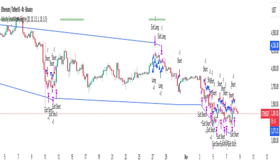
Velocity SmartMoney Engine work - Delta Exchange📈 Velocity SmartMoney Engine
Adaptive Breakout & Order Block Strategy with Dynamic Risk Control
---
🔍 Overview
The Velocity SmartMoney Engine is a next-generation trading strategy that fuses Smart Money breakout logic , Order Block structure detection , and Supertrend-based directional filtering into one precision-built system.
It identifies institutional-level breakouts , manages positions with ATR-based adaptive risk , and executes disciplined exits using stop-loss, trailing stop, and profit target logic.
Designed for swing and short-term system traders, this strategy performs excellently on BTC, ETH, NIFTY, BANKNIFTY, Gold, and major FX pairs — best on 15m to 4h timeframes .
---
⚙️ Core Components
1️⃣ Smart Money Breakout Logic
Detects real breakouts using dynamic support/resistance pivots.
Confirms entries only during strong volatility bursts.
Avoids false breakouts in sideways markets.
2️⃣ Order Block Gap Detection
Finds institutional imbalance zones (Smart Money footprints).
Bullish gaps = Long bias; Bearish gaps = Short bias.
Works with candle confirmation and momentum validation.
3️⃣ Supertrend Directional Filter
Trades only in direction of Supertrend bias.
Exits instantly when Supertrend flips.
Prevents entries against dominant trend.
4️⃣ ATR-Based Risk & Volatility Filter
Uses ATR × multiplier for adaptive stop sizing.
Volatility filter ensures trades trigger only during active markets.
Avoids whipsaw zones.
---
💰 Position Management
Stop-Loss: Adaptive ATR-based.
Take-Profit: Default 5% target (editable input).
Trailing Stop: Auto-adjusts to lock profits.
No-Exit Hold: Hold position for defined candles before exits.
Supertrend Flip Exit: Instant trend-based closure.
---
🧠 Built-In Trade Discipline
One-trade-per-bar guard prevents duplicate entries.
Volatility-weighted breakout validation.
Clean and conflict-free exit hierarchy.
---
🎯 Key Features
✅ Smart Money breakout + Order Block fusion
✅ Supertrend-based trend confirmation
✅ ATR dynamic stop + 5% profit target
✅ Adaptive trailing logic
✅ One-trade-per-bar control
✅ Works across Crypto, Indices, FX, Commodities
✅ Ideal for 1h–4h swing setups
---
📊 Recommended Settings
Parameter | Typical Value | Purpose
--- | --- | ---
Levels Period | 20 | Pivot lookback for S/R zones
Volatility Filter | 20–40 | Filters out low-momentum areas
ATR Multiplier | 1.5 | Adjust stop size by volatility
Supertrend Length | 10 | ATR period for trend bias
Supertrend Multiplier | 3.0 | Supertrend sensitivity
Target Profit | 5% | Default take-profit level
---
⚡ Suggested Use
• Best suited for swing entries on 1H / 4H charts .
• Combine with session filters or trend confluence for automation.
• Ideal as a base module for TradingView + Broker integrations .
---
🧩 Disclaimer
This script is for educational purposes only .
Past performance does not guarantee future returns.
Use responsibly. The developer assumes no liability for financial losses.
---
💬 Community & Access
Developed by: Shubham Singh
Version: Velocity SmartMoney Engine v1.0
For premium modules & automation: DM "Velocity Access" on chat to request access.
---
© 2025 Velocity SmartMoney Engine — All Rights Reserved
TitanEdge Algo Suite — 4H BTC & ETH (Delta Exchange Ready)TitanEdge Algo Suite — 4H BTC & ETH (Delta Exchange Ready)
TitanEdge Algo Suite is a next-generation trading system that fuses volatility-adaptive logic, order-block structure, SuperTrend direction filtering, and ATR-based exits into a single modular framework.
It’s engineered for 4-hour BTC and ETH swing trading, delivering institutional-grade entries, dynamic risk control, and precise exits.
⚙️ Core Features
1. Volatility Oscillator (0–100)
• Filters trades by volatility intensity.
• Uses ATR, Range, or Bollinger Band Width normalization.
• Trades trigger only when market volatility is high — filtering out sideways or weak trends.
• Ensures trades occur during real momentum expansions.
2. Breakout + Order Block Engine
• Detects pivot highs/lows to confirm authentic breakout levels.
• Identifies “smart money” gaps — institutional imbalance zones often leading to strong reversals or continuations.
• Captures both breakout continuations and order-block reversals.
• Works as a hybrid structure detector combining price action and volatility alignment.
3. SuperTrend Directional Filter
• Optional filter that only allows trades in the direction of the SuperTrend.
• Can automatically close trades when a SuperTrend flip occurs.
• Provides strong trend-following bias and helps avoid countertrend traps.
4. ATR-Based Stop & Trailing System
• Adaptive stop-loss and trailing logic that expands or tightens based on volatility.
• Supports three modes: StopOnly, TrailOnly, and StopAndTrail.
• Works in both ATR-based distance or percentage-based configuration.
• Keeps losing trades small and lets winning trades extend dynamically.
5. Volume-Based Exit Logic
• Detects low-volume exhaustion to identify momentum loss.
• Detects opposite-volume spikes as early reversal signals.
• Optional hybrid “Both” mode combines both detection methods for stronger reliability.
• Ideal for markets where volume surges indicate smart money exits or trap formations.
6. Session Filter & Anti-Churn Control
• Restrict trading hours (optional; not required for crypto).
• Prevents repeated signals and noise-based entries through minimum bars between trades.
• Cooldown logic ensures disciplined trading and avoids strategy overlap.
• Prevents multiple entries in a single bar and filters unconfirmed breakouts.
7. SmartMoney Preset Mode
• Institutional-grade configuration automatically adjusting volatility, ATR, and structural logic.
• Mimics smart money behavior by prioritizing clean structure and high liquidity volatility zones.
• Great for traders who want simplified institutional logic without manual tuning.
Optimized for 4H BTC & ETH
TitanEdge performs best on BTCUSDT and ETHUSDT pairs in the 4-hour timeframe.
The 4H chart captures high-volatility institutional swings, eliminates intraday noise, and provides clear order-block setups.
This timeframe aligns with BTC/ETH volatility cycles, providing consistent signals and cleaner trend confirmation.
Recommended settings for 4H charts:
• Levels Period: 25
• Volatility Filter: 20
• volatility oscillator Auto: disable ( it depend upon your plan test with Disable/enable)
• Volatility Method: BBWidth
• ATR Multiplier: 1.8
• ATR Stop %: 5
• SuperTrend ATR Length: 10
• SuperTrend Factor: 3
• ATR Mode: StopAndTrail
• Hold Bars: 1
• Volume Exit: Disable (Both)
• Session Filter: Off (Crypto runs 24/7)
Entry Logic
• Long Entry: Price breaks above resistance (pivot high), volatility above threshold, and optional SuperTrend confirmation.
• Short Entry: Price breaks below support (pivot low), volatility above threshold, and optional bearish SuperTrend confirmation.
• Additional Entry: Triggered by order-block gaps (smart money imbalances) in volatility expansion phases.
• Trades only when both direction and volatility align to ensure precision entries.
Exit Logic
• ATR Stop and Trail dynamically manage open trades.
• SuperTrend Flip forces exit on trend reversal.
• Volume Exit triggers when volume momentum drops or opposite spike occurs.
• Optional session close exit to flatten trades outside hours.
• Logic prevents premature exits with “Hold Bars” delay after entry.
Why You Need TitanEdge Algo Suite
• Trades only during high-volatility, strong-momentum phases — no false breakouts or choppy trades.
• ATR risk control automatically adjusts to each market’s volatility conditions.
• Identifies institutional order-blocks and clean breakouts for precise entries.
• SuperTrend filter adds directional bias, boosting win-rate consistency.
• Volume exit logic ensures profits are protected when market momentum fades.
• Works 24/7 across all major crypto pairs — fully automated and customizable.
• Built for 4H swing trades — fewer but higher-quality setups.
• Fully compatible with TradingView alerts and bot integration for hands-free execution.
How TitanEdge Makes Profit
• TitanEdge only trades during volatility expansion, when breakout continuation probability is statistically high.
• ATR dynamic stops prevent large losses by scaling protection according to real volatility.
• Trend filtering keeps positions aligned with major market flows.
• Order-block detection ensures entries are based on price structure rather than random signals.
• Volume-based exits secure profits early when momentum weakens.
• SmartMoney Preset provides optimal balance between trade frequency, accuracy, and drawdown control.
• The system compounds edge by maintaining trade discipline — fewer but stronger trades over time.
Delta Exchange Integration (TradingView Bot Ready)
TitanEdge is fully compatible with TradingView alert webhooks and can connect to Delta Exchange or any bot-supported broker.
Alert JSON message format:
{"symbol":"{{ticker}}","side":"{{strategy.order.action}}","qty":1,"trigger_time":"{{timenow}}","strategy_id":"code"}
qty 1 represent 1 lot so if you want to take trade with 5 lots or 0.05eth and write
{"symbol":"{{ticker}}","side":"{{strategy.order.action}}","qty":5,"trigger_time":"{{timenow}}","strategy_id":"code"}
Steps to automate:
Create an alert on TradingView using “Once Per Bar Close”.
Paste your bot or automation webhook URL.
Paste the JSON above as the message.
Configure your bot or API bridge (like PineConnector, AutoView, or WunderTrading) to route signals to Delta Exchange.
On Delta, use BTCUSD or ETHUSD Perpetual pairs with moderate leverage (3x–5x).
Enable Cross Margin for smooth drawdown handling.
Test first on Delta Testnet for safety.
Why 4H BTC & ETH Works Best
• 4H candles capture true volatility swings and filter lower-timeframe noise.
• Aligns with institutional liquidity cycles in BTC and ETH.
• ATR and volume-based stops perform optimally on larger bars.
• Smoother equity curve and less drawdown compared to intraday trading.
• Ideal for traders seeking structured, medium-term trades with high reward-to-risk.
Unique Edge
• Combines breakout, order-block, and volatility principles into one adaptive model.
• Incorporates volatility normalization (ATR/BBWidth) for multi-market adaptability.
• Dynamic ATR stops and trailing protect capital during unstable phases.
• Volume and trend exits create layered protection systems.
• 4H optimization eliminates noise and provides clear institutional alignment.
• SmartMoney preset auto-configures settings to mimic large-player behavior.
• Fully automated via webhooks — no manual execution required.
• Modular design lets you customize each component for different trading styles.
TradingView Bot Integration
TitanEdge is fully plug-and-play with all TradingView-compatible bots.
Each alert sends structured JSON data containing direction, symbol, and quantity, ready for execution on your connected broker.
You can route the data to:
• PineConnector (MT4/MT5 bridge)
• WunderTrading
• AutoView
• Custom Node/REST API handler
This makes TitanEdge a professional-grade strategy suitable for semi-automatic or fully automated crypto trading setups.
Professional Recommendations
• Timeframe: 4H
• Instruments: BTCUSDT, ETHUSDT
• Exchange: Delta Exchange (Perpetual Futures)
• Leverage: 3x–5x
• Session Filter: Off (crypto 24/7)
• Risk per trade: 0.5%–1% of total equity
• Alert Type: Once Per Bar Close
• Volatility Filter: 25–35 depending on market activity
• Always use realistic slippage and fees for backtests.
Summary
TitanEdge Algo Suite is a complete trading framework built to deliver institutional-quality precision with full automation support.
It captures powerful volatility expansions on 4H BTC and ETH charts using clean structure, adaptive stops, and directional trend filters.
Every feature — from entry logic to exits — is designed to protect capital and amplify performance through disciplined, volatility-aware execution.
TitanEdge is not just another script — it’s a professional-grade algorithm that combines volatility intelligence, structural precision, and adaptive risk control.
TitanEdge Algo Suite = Smart Logic × Trend Discipline × Adaptive Risk Control
Optimized for BTC & ETH on 4H charts. Built for traders who demand precision, control, and consistency.

ORB Breakout Strategy w/ Filters - Dynamic Sizing - MTFHere is a comprehensive description of the strategy, written in a clear and structured format. You can use this for your script's "how-to-use" guide or documentation.
---
## 📈 Opening Range Breakout (ORB) Strategy
This is a comprehensive, multi-timeframe strategy built for trading opening range breakouts. It is designed with a "filters-first" approach, allowing you to validate a breakout with trend, volume, and volatility.
The strategy's core power comes from its flexibility. You can trade on a low timeframe (like a 1-minute chart) while basing your breakout levels on a higher timeframe's opening bar (e.g., the first 15-minute bar). It includes dynamic position sizing based on risk and a wide array of advanced exit management options.
### Key Features
* **Multi-Timeframe Opening Range:** The core of the strategy. You can define the "Opening Range" timeframe (5, 10, 15, 30, or 60 min) *independently* of your chart timeframe.
* **Custom Trading Session:** Define the exact session (e.g., "0930-1600" in "America/New_York") you want to trade.
* **One Trade Per Session:** The strategy will only take the *first valid breakout* signal per day to avoid over-trading.
---
### 🚦 Entry Signals & Filters
A trade is only initiated when the price closes above the Session High or below the Session Low **AND** all active filters are passed.
* **Trend Filter:** (Optional) Requires price to be above a long-term MA (e.g., 100 EMA) for long trades and below it for short trades.
* **Volume Filter:** (Optional) Requires the breakout bar's volume to be a specified multiplier (e.g., 1.5x) of the recent average volume.
* **Volatility Filter:** (Optional) Requires the current ATR to be higher than its long-term average, ensuring you only trade during periods of expanding volatility.
* **Direction Filter:** Allows you to isolate the strategy to **Long Only**, **Short Only**, or **Both**.
---
### 💰 Dynamic Position Sizing
The strategy includes a robust "Risk %" sizing model.
* **Risk-Based Sizing:** Instead of fixed contracts, it calculates the position size based on your **Account Size**, **Risk % per Trade**, and the **Stop Loss distance**.
* **Auto-Detect Point Value:** It automatically detects the correct point value for popular futures contracts (ES, NQ, MES, MNQ) and provides a manual override for other assets.
---
### 📤 Exit & Risk Management
This strategy features a multi-layered exit system, giving you complete control over how trades are managed.
#### 1. Stop Loss (SL)
Your initial stop loss can be calculated using a fixed **Tick** offset or an **ATR** multiplier. It can be anchored from two different points:
* **Breakout Level:** The stop is placed relative to the `sessionHigh` or `sessionLow` level.
* **Entry Bar:** The stop is placed relative to the high/low of the bar that *triggered* the entry.
#### 2. Take Profit (TP)
A standard Take Profit can be set using a fixed **Tick** offset or an **ATR** multiplier.
#### 3. Advanced Exit Logic
These options override the standard Take Profit to allow for more dynamic trade management:
* **Trailing Take Profit (TTP):**
* **Fixed/ATR Trail:** A standard trailing stop that activates after price moves a certain amount in your favor.
* **MA Price Cross:** Exits the trade as soon as the price closes across a fast-moving average (e.g., 9-EMA).
* **MA Crossover:** Exits the trade as soon as a fast MA crosses below a slow MA (for longs) or above (for shorts).
* **Close on Reversal:** (Optional) Exits immediately if the **very next bar** after entry closes back *inside* the opening range (a "failed breakout" signal).
* **Close on Opposite Range Cross:** (Optional) Exits a long trade if the price ever closes below the `sessionLow` (and vice-versa for shorts).
* **End of Session Exit:** All open positions are automatically closed at the end of the defined trading session.

ScalpMaster – Breaker BlocksIdeal for scalpers📈and intraday traders who rely on breaker-block reactions and market-structure shifts to refine entries and exits.
Add it to your chart, enable alerts for Signal UP and Signal DN, and combine with your own bias or higher-timeframe analysis.
✅ Automatic breaker-block detection (+BB / –BB)
✅ Real-time signal UP / signal DN
✅ Market-structure swing and PD Array visualization
✅ Optional take-profit targets (R:R zones)
✅ Alert conditions for every signal event
✅ Works on any timeframe & asset

OG Trend MasterOG Trend Master
Smart trend-tracking indicator designed to identify opportunities using Supertrend + EMA confirmation logic.
It automatically adapts to market volatility and structure:
✅ Supertrend core to detect directional bias
⚡ Dual EMA cross for confirmation and precision
🎯 Visual arrows + diamonds for instant clarity on entries
🔔 Real-time alerts for both LONG and SHORT confirmations
Built for traders who value simplicity, accuracy, and flow.
From scalpers to swing traders OG Trend Master delivers smooth trend identification across all timeframes.

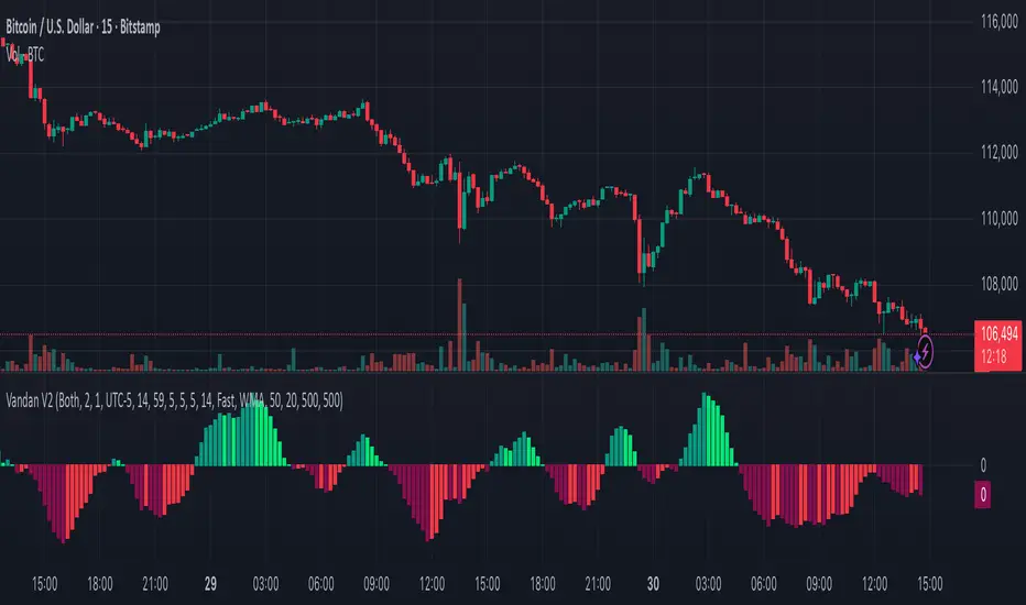
Vandan V2Vandan V2 is an automated trend-following strategy for NASDAQ E-mini Futures (NQ1!).
It uses multi-timeframe momentum and volatility filters to identify high-probability entries.
Includes dynamic risk management and trailing logic optimized for intraday trading.
Algoritmictrader2025 ALGO System profitability works with a minimum profit margin of 75% and the maximum profit margin per share is around 95%. The software costs $150 per month.

One For All Strategy by Anson🏆 Exclusive Indicator: One For All Strategy
.
📈 Works for stocks, forex, crypto, indices
📈 Easy to use, real-time alerts, no repaint
📈 No grid, no martingale, no hedging
📈 One position at a time
.
One For All Strategy by Anson
A multi-indicator TradingView strategy designed to identify long and short trading opportunities by combining trend-following and momentum signals, paired with risk management rules to guide entries and exits.
.
Core Logic & Key Indicator:
X Moving Average: A proprietary adaptive moving average that adjusts its responsiveness to price changes based on market volatility. It uses an efficiency ratio to modify its smoothing behavior—adapting to whether the market is trending or ranging. Users can toggle a setting to let this ratio dynamically adjust the indicator’s sensitivity or use a fixed smoothing factor.
.
Entry Conditions:
.
Long Entry: Triggered when momentum signals strength, price action aligns with a broader upward trend, the X MA indicates short-term upward momentum, and a minimum number of bars have passed since the last trade (to prevent overtrading).
.
Short Entry: Triggered when momentum signals weakness, price action aligns with a broader downward trend, the X MA indicates short-term downward momentum, and a minimum number of bars have passed since the last trade.
.
Exit Conditions:
.
Trailing Stop: Activates after a position has been open for a set number of bars (to avoid premature exits). A trailing stop—based on a percentage of the entry price—locks in profits as the trade moves favorably, adjusting dynamically to protect gains.
.
Additional Features:
Visualisation: Overlays the X MA (orange line) and price (semi-transparent blue) on the chart for clear signal tracking.
.
See the author's instructions on the right to learn how to get access to the strategy.

DayFlow VWAP Relay Forex Majors StrategySummary in one paragraph
DayFlow VWAP Relay is a day-trading strategy for major FX pairs on intraday timeframes, demonstrated on EURUSD 15 minutes. It waits for alignment between a daily anchored VWAP regime check, residual percentiles, and lower-timeframe micro flow before suggesting trades. The originality is the fusion of daily VWAP residual percentiles with a live micro-flow score from 1 minute data to switch between fade and breakout behavior inside the same session. Add it to a clean chart and use the markers and alerts.
Scope and intent
• Markets: Major FX pairs such as EURUSD, GBPUSD, USDJPY, AUDUSD, USDCHF, USDCAD
• Timeframes: One minute to one hour
• Default demo in this publication: EURUSD on 15 minutes
• Purpose: Reduce false starts by acting only when context, location and micro flow agree
• Limits: This is a strategy. Orders are simulated on standard candles only
Originality and usefulness
• Core novelty: Residual percentiles to daily anchored VWAP decide “balanced versus expanding day”. A separate 1 minute micro-flow score confirms direction, so the same model fades extremes in balance and rides range breaks in expansion
• Failure modes addressed: Chop fakeouts and unconfirmed breakouts are filtered by the expansion gate and micro-flow threshold
• Testability: Every input is exposed. Bands, background regime color, and markers show why a suggestion appears
• Portable yardstick: Stops and targets are ATR multiples converted to ticks, which transfer across symbols
• Open source status: No reused third-party code that requires attribution
Method overview in plain language
The day is anchored with a VWAP that updates from the daily session start. Price minus VWAP is the residual. Percentiles of that residual measured over a rolling window define location extremes for the current day. A regime score compares residual volatility to price volatility. When expansion is low, the day is treated as balanced and the model fades residual extremes if 1 minute micro flow points back to VWAP. When expansion is high, the model trades breakouts outside the VWAP bands if slope and micro flow agree with the move.
Base measures
• Range basis: True Range smoothed by ATR for stops and targets, length 14
• Return basis: Not required for signals; residuals are absolute price distance to VWAP
Components
• Daily Anchor VWAP Bands. VWAP with standard-deviation bands. Slope sign is used for trend confirmation on breakouts
• Residual Percentiles. Rolling percentiles of close minus VWAP over Signal length. Identify location extremes inside the day
• Expansion Ratio. Standard deviation of residuals divided by standard deviation of price over Signal length. Classifies balanced versus expanding day
• Micro Flow. Net up minus down closes from 1 minute data across a short span, normalized to −1..+1. Confirms direction and avoids fades against pressure
• Session Window optional. Restricts trading to your configured hours to avoid thin periods
• Cooldown optional. Bars to wait after a position closes to prevent immediate re-entry
Fusion rule
Gating rather than weighting. First choose regime by Expansion Ratio versus the Expansion gate. Inside each regime all listed conditions must be true: location test plus micro-flow threshold plus session window plus cooldown. Breakouts also require VWAP slope alignment.
Signal rule
• Long suggestion on balanced day: residual at or below the lower percentile and micro flow positive above the gate while inside session and cooldown is satisfied
• Short suggestion on balanced day: residual at or above the upper percentile and micro flow negative below the gate while inside session and cooldown is satisfied
• Long suggestion on expanding day: close above the upper VWAP band, VWAP slope positive, micro flow positive, session and cooldown satisfied
• Short suggestion on expanding day: close below the lower VWAP band, VWAP slope negative, micro flow negative, session and cooldown satisfied
• Positions flip on opposite suggestions or exit by brackets
What you will see on the chart
• Markers on suggestion bars: L for long, S for short
• Exit occurs on reverse signal or when a bracket order is filled
• Reference lines: daily anchored VWAP with upper and lower bands
• Optional background: teal for balanced day, orange for expanding day
Inputs with guidance
Setup
• Signal length. Residual and regime window. Typical 40 to 100. Higher smooths, lower reacts faster
Micro Flow
• Micro TF. Lower timeframe used for micro flow, default 1 minute
• Micro span bars. Count of lower-TF bars. Typical 5 to 20
• Micro flow gate 0..1. Minimum absolute flow. Raising it demands stronger confirmation and reduces trade count
VWAP Bands
• VWAP stdev multiplier. Band width. Typical 0.8 to 1.6. Wider bands reduce breakout frequency and increase fade distance
• Expansion gate 0..3. Threshold to switch from fades to breakouts. Raising it favors fades, lowering it favors breakouts
Sessions
• Use session filter. Enable to trade only inside your window
• Trade window UTC. Default 07:00 to 17:00
Risk
• ATR length. Stop and target basis. Typical 10 to 21
• Stop ATR x. Initial stop distance in ATR multiples
• Target ATR x. Profit target distance in ATR multiples
• Cooldown bars after close. Wait bars before a new entry
• Side. Both, long only, or short only
View
• Show VWAP and bands
• Color bars by residual regime
Properties visible in this publication
• Initial capital 10000
• Base currency Default
• request.security uses lookahead off everywhere
• Strategy: Percent of equity with value 3. Pyramiding 0. Commission cash per order 0.0001 USD. Slippage 3 ticks. Process orders on close ON. Bar magnifier ON. Recalculate after order is filled OFF. Calc on every tick OFF. Using standard OHLC fills ON.
Realism and responsible publication
No performance claims. Past results never guarantee future outcomes. Fills and slippage vary by venue. Shapes can move while a bar forms and settle on close. Strategies must run on standard candles for signals and orders.
Honest limitations and failure modes
High impact news, session opens, and thin liquidity can invalidate assumptions. Very quiet days can reduce contrast between residuals and price volatility. Session windows use the chart exchange time. If both stop and target are touched within a single bar, TradingView’s standard OHLC price-movement model decides the outcome.
Expect different behavior on illiquid pairs or during holidays. The model is sensitive to session definitions and feed time. Past results never guarantee future outcomes.
Legal
Education and research only. Not investment advice. You are responsible for your decisions. Test on historical data and in simulation before any live use. Use realistic costs.

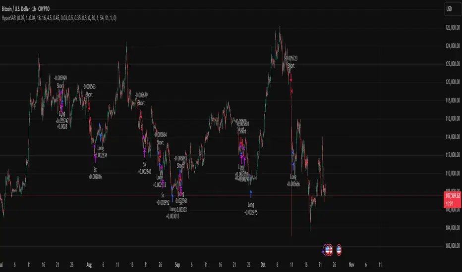
Hyper SAR Reactor Trend StrategyHyperSAR Reactor Adaptive PSAR Strategy
Summary
Adaptive Parabolic SAR strategy for liquid stocks, ETFs, futures, and crypto across intraday to daily timeframes. It acts only when an adaptive trail flips and confirmation gates agree. Originality comes from a logistic boost of the SAR acceleration using drift versus ATR, plus ATR hysteresis, inertia on the trail, and a bear-only gate for shorts. Add to a clean chart and run on bar close for conservative alerts.
Scope and intent
• Markets: large cap equities and ETFs, index futures, major FX, liquid crypto
• Timeframes: one minute to daily
• Default demo: BTC on 60 minute
• Purpose: faster yet calmer PSAR that resists chop and improves short discipline
• Limits: this is a strategy that places simulated orders on standard candles
Originality and usefulness
• Novel fusion: PSAR AF is boosted by a logistic function of normalized drift, trail is monotone with inertia, entries use ATR buffers and optional cooldown, shorts are allowed only in a bear bias
• Addresses false flips in low volatility and weak downtrends
• All controls are exposed in Inputs for testability
• Yardstick: ATR normalizes drift so settings port across symbols
• Open source. No links. No solicitation
Method overview
Components
• Adaptive AF: base step plus boost factor times logistic strength
• Trail inertia: one sided blend that keeps the SAR monotone
• Flip hysteresis: price must clear SAR by a buffer times ATR
• Volatility gate: ATR over its mean must exceed a ratio
• Bear bias for shorts: price below EMA of length 91 with negative slope window 54
• Cooldown bars optional after any entry
• Visual SAR smoothing is cosmetic and does not drive orders
Fusion rule
Entry requires the internal flip plus all enabled gates. No weighted scores.
Signal rule
• Long when trend flips up and close is above SAR plus buffer times ATR and gates pass
• Short when trend flips down and close is below SAR minus buffer times ATR and gates pass
• Exit uses SAR as stop and optional ATR take profit per side
Inputs with guidance
Reactor Engine
• Start AF 0.02. Lower slows new trends. Higher reacts quicker
• Max AF 1. Typical 0.2 to 1. Caps acceleration
• Base step 0.04. Typical 0.01 to 0.08. Raises speed in trends
• Strength window 18. Typical 10 to 40. Drift estimation window
• ATR length 16. Typical 10 to 30. Volatility unit
• Strength gain 4.5. Typical 2 to 6. Steepness of logistic
• Strength center 0.45. Typical 0.3 to 0.8. Midpoint of logistic
• Boost factor 0.03. Typical 0.01 to 0.08. Adds to step when strength rises
• AF smoothing 0.50. Typical 0.2 to 0.7. Adds inertia to AF growth
• Trail smoothing 0.35. Typical 0.15 to 0.45. Adds inertia to the trail
• Allow Long, Allow Short toggles
Trade Filters
• Flip confirm buffer ATR 0.50. Typical 0.2 to 0.8. Raise to cut flips
• Cooldown bars after entry 0. Typical 0 to 8. Blocks re entry for N bars
• Vol gate length 30 and Vol gate ratio 1. Raise ratio to trade only in active regimes
• Gate shorts by bear regime ON. Bear bias window 54 and Bias MA length 91 tune strictness
Risk
• TP long ATR 1.0. Set to zero to disable
• TP short ATR 0.0. Set to 0.8 to 1.2 for quicker shorts
Usage recipes
Intraday trend focus
Confirm buffer 0.35 to 0.5. Cooldown 2 to 4. Vol gate ratio 1.1. Shorts gated by bear regime.
Intraday mean reversion focus
Confirm buffer 0.6 to 0.8. Cooldown 4 to 6. Lower boost factor. Leave shorts gated.
Swing continuation
Strength window 24 to 34. ATR length 20 to 30. Confirm buffer 0.4 to 0.6. Use daily or four hour charts.
Properties visible in this publication
Initial capital 10000. Base currency USD. Order size Percent of equity 3. Pyramiding 0. Commission 0.05 percent. Slippage 5 ticks. Process orders on close OFF. Bar magnifier OFF. Recalculate after order filled OFF. Calc on every tick OFF. No security calls.
Realism and responsible publication
No performance claims. Past results never guarantee future outcomes. Shapes can move while a bar forms and settle on close. Strategies execute only on standard candles.
Honest limitations and failure modes
High impact events and thin books can void assumptions. Gap heavy symbols may prefer longer ATR. Very quiet regimes can reduce contrast and invite false flips.
Open source reuse and credits
Public domain building blocks used: PSAR concept and ATR. Implementation and fusion are original. No borrowed code from other authors.
Strategy notice
Orders are simulated on standard candles. No lookahead.
Entries and exits
Long: flip up plus ATR buffer and all gates true
Short: flip down plus ATR buffer and gates true with bear bias when enabled
Exit: SAR stop per side, optional ATR take profit, optional cooldown after entry
Tie handling: stop first if both stop and target could fill in one bar
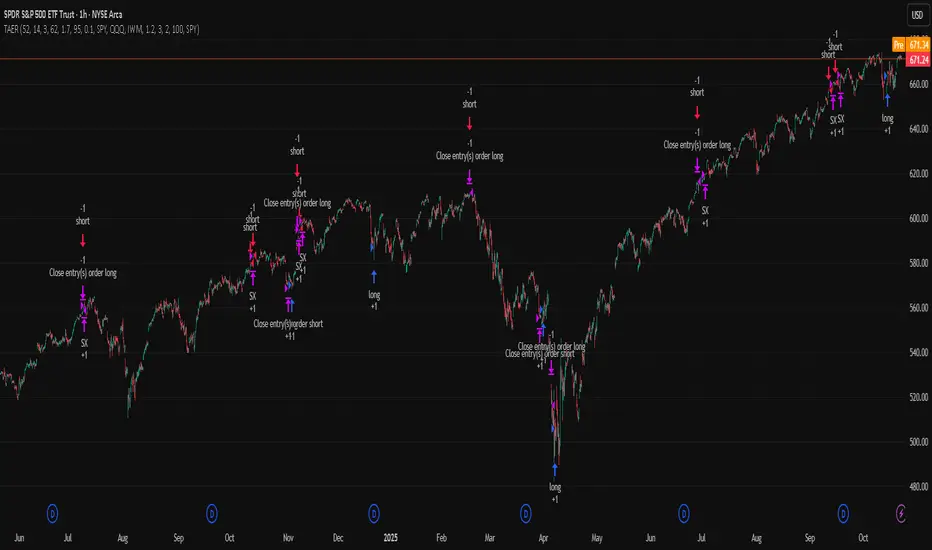
TriAnchor Elastic Reversion US Market SPY and QQQ adaptedSummary in one paragraph
Mean-reversion strategy for liquid ETFs, index futures, large-cap equities, and major crypto on intraday to daily timeframes. It waits for three anchored VWAP stretches to become statistically extreme, aligns with bar-shape and breadth, and fades the move. Originality comes from fusing daily, weekly, and monthly AVWAP distances into a single ATR-normalized energy percentile, then gating with a robust Z-score and a session-safe gap filter.
Scope and intent
• Markets: SPY QQQ IWM NDX large caps liquid futures liquid crypto
• Timeframes: 5 min to 1 day
• Default demo: SPY on 60 min
• Purpose: fade stretched moves only when multi-anchor context and breadth agree
• Limits: strategy uses standard candles for signals and orders only
Originality and usefulness
• Unique fusion: tri-anchor AVWAP energy percentile plus robust Z of close plus shape-in-range gate plus breadth Z of SPY QQQ IWM
• Failure mode addressed: chasing extended moves and fading during index-wide thrusts
• Testability: each component is an input and visible in orders list via L and S tags
• Portable yardstick: distances are ATR-normalized so thresholds transfer across symbols
• Open source: method and implementation are disclosed for community review
Method overview in plain language
Base measures
• Range basis: ATR(length = atr_len) as the normalization unit
• Return basis: not used directly; we use rank statistics for stability
Components
• Tri-Anchor Energy: squared distances of price from daily, weekly, monthly AVWAPs, each divided by ATR, then summed and ranked to a percentile over base_len
• Robust Z of Close: median and MAD based Z to avoid outliers
• Shape Gate: position of close inside bar range to require capitulation for longs and exhaustion for shorts
• Breadth Gate: average robust Z of SPY QQQ IWM to avoid fading when the tape is one-sided
• Gap Shock: skip signals after large session gaps
Fusion rule
• All required gates must be true: Energy ≥ energy_trig_prc, |Robust Z| ≥ z_trig, Shape satisfied, Breadth confirmed, Gap filter clear
Signal rule
• Long: energy extreme, Z negative beyond threshold, close near bar low, breadth Z ≤ −breadth_z_ok
• Short: energy extreme, Z positive beyond threshold, close near bar high, breadth Z ≥ +breadth_z_ok
What you will see on the chart
• Standard strategy arrows for entries and exits
• Optional short-side brackets: ATR stop and ATR take profit if enabled
Inputs with guidance
Setup
• Base length: window for percentile ranks and medians. Typical 40 to 80. Longer smooths, shorter reacts.
• ATR length: normalization unit. Typical 10 to 20. Higher reduces noise.
• VWAP band stdev: volatility bands for anchors. Typical 2.0 to 4.0.
• Robust Z window: 40 to 100. Larger for stability.
• Robust Z entry magnitude: 1.2 to 2.2. Higher means stronger extremes only.
• Energy percentile trigger: 90 to 99.5. Higher limits signals to rare stretches.
• Bar close in range gate long: 0.05 to 0.25. Larger requires deeper capitulation for longs.
Regime and Breadth
• Use breadth gate: on when trading indices or broad ETFs.
• Breadth Z confirm magnitude: 0.8 to 1.8. Higher avoids fighting thrusts.
• Gap shock percent: 1.0 to 5.0. Larger allows more gaps to trade.
Risk — Short only
• Enable short SL TP: on to bracket shorts.
• Short ATR stop mult: 1.0 to 3.0.
• Short ATR take profit mult: 1.0 to 6.0.
Properties visible in this publication
• Initial capital: 25000USD
• Default order size: Percent of total equity 3%
• Pyramiding: 0
• Commission: 0.03 percent
• Slippage: 5 ticks
• Process orders on close: OFF
• Bar magnifier: OFF
• Recalculate after order is filled: OFF
• Calc on every tick: OFF
• request.security lookahead off where used
Realism and responsible publication
• No performance claims. Past results never guarantee future outcomes
• Fills and slippage vary by venue
• Shapes can move during bar formation and settle on close
• Standard candles only for strategies
Honest limitations and failure modes
• Economic releases or very thin liquidity can overwhelm mean-reversion logic
• Heavy gap regimes may require larger gap filter or TR-based tuning
• Very quiet regimes reduce signal contrast; extend windows or raise thresholds
Open source reuse and credits
• None
Strategy notice
Orders are simulated by TradingView on standard candles. request.security uses lookahead off where applicable. Non-standard charts are not supported for execution.
Entries and exits
• Entry logic: as in Signal rule above
• Exit logic: short side optional ATR stop and ATR take profit via brackets; long side closes on opposite setup
• Risk model: ATR-based brackets on shorts when enabled
• Tie handling: stop first when both could be touched inside one bar
Dataset and sample size
• Test across your visible history. For robust inference prefer 100 plus trades.
Aurum DCX AVE Gold and Silver StrategySummary in one paragraph
Aurum DCX AVE is a volatility break strategy for gold and silver on intraday and swing timeframes. It aligns a new Directional Convexity Index with an Adaptive Volatility Envelope and an optional USD/DXY bias so trades appear only when direction quality and expansion agree. It is original because it fuses three pieces rarely combined in one model for metals: a convexity aware trend strength score, a percentile based envelope that widens with regime heat, and an intermarket DXY filter.
Scope and intent
• Markets. Gold and silver futures or spot, other liquid commodities, major indices
• Timeframes. Five minutes to one day. Defaults to 30min for swing pace
• Default demo used in this publication. TVC:GOLD on 30m
• Purpose. Enter confirmed volatility breaks while muting chop using regime heat and USD bias
• Limits. This is a strategy. Orders are simulated on standard candles only
Originality and usefulness
• Unique fusion. DCX combines DI strength with path efficiency and curvature. AVE blends ATR with a high TR percentile and widens with DCX heat. DXY adds an intermarket bias
• Failure mode addressed. False starts inside compression and unconfirmed breakouts during USD swings
• Testability. Each component has a named input. Entry names L and S are visible in the list of trades
• Portable yardstick. Weekly ATR for stops and R multiples for targets
• Open source. Method and implementation are disclosed for community review
Method overview in plain language
You score direction quality with DCX, size an adaptive envelope with a blend of ATR and a high TR percentile, and only allow breaks that clear the band while DCX is above a heat threshold in the same direction. An optional DXY filter favors long when USD weakens and short when USD strengthens. Orders are bracketed with a Weekly ATR stop and an R multiple target, with optional trailing to the envelope.
Base measures
• Range basis. True Range and ATR over user windows. A high TR percentile captures expansion tails used by AVE
• Return basis. Not required
Components
• Directional Convexity Index DCX. Measures directional strength with DX, multiplies by path efficiency, blends a curvature term from acceleration, scales to 0 to 100, and uses a rise window
• Adaptive Volatility Envelope AVE. Midline ALMA or HMA or EMA plus bands sized by a blend of ATR and a high TR percentile. The blend weight follows volatility of volatility. Band width widens with DCX heat
• DXY Bias optional. Daily EMA trend of DXY. Long bias when USD weakens. Short bias when USD strengthens
• Risk block. Initial stop equals Weekly ATR times a multiplier. Target equals an R multiple of the initial risk. Optional trailing to AVE band
Fusion rule
• All gates must pass. DCX above threshold and rising. Directional lead agrees. Price breaks the AVE band in the same direction. DXY bias agrees when enabled
Signal rule
• Long. Close above AVE upper and DCX above threshold and DCX rising and plus DI leads and DXY bias is bearish
• Short. Close below AVE lower and DCX above threshold and DCX falling and minus DI leads and DXY bias is bullish
• Exit and flip. Bracket exit at stop or target. Optional trailing to AVE band
Inputs with guidance
Setup
• Symbol. Default TVC:GOLD (Correlation Asset for internal logic)
• Signal timeframe. Blank follows the chart
• Confirm timeframe. Default 1 day used by the bias block
Directional Convexity Index
• DCX window. Typical 10 to 21. Higher filters more. Lower reacts earlier
• DCX rise bars. Typical 3 to 6. Higher demands continuation
• DCX entry threshold. Typical 15 to 35. Higher avoids soft moves
• Efficiency floor. Typical 0.02 to 0.06. Stability in quiet tape
• Convexity weight 0..1. Typical 0.25 to 0.50. Higher gives curvature more influence
Adaptive Volatility Envelope
• AVE window. Typical 24 to 48. Higher smooths more
• Midline type. ALMA or HMA or EMA per preference
• TR percentile 0..100. Typical 75 to 90. Higher favors only strong expansions
• Vol of vol reference. Typical 0.05 to 0.30. Controls how much the percentile term weighs against ATR
• Base envelope mult. Typical 1.4 to 2.2. Width of bands
• Regime adapt 0..1. Typical 0.6 to 0.95. How much DCX heat widens or narrows the bands
Intermarket Bias
• Use DXY bias. Default ON
• DXY timeframe. Default 1 day
• DXY trend window. Typical 10 to 50
Risk
• Risk percent per trade. Reporting field. Keep live risk near one to two percent
• Weekly ATR. Default 14. Basis for stops
• Stop ATR weekly mult. Typical 1.5 to 3.0
• Take profit R multiple. Typical 1.5 to 3.0
• Trail with AVE band. Optional. OFF by default
Properties visible in this publication
• Initial capital. 20000
• Base currency. USD
• request.security lookahead off everywhere
• Commission. 0.03 percent
• Slippage. 5 ticks
• Default order size method percent of equity with value 3% of the total capital available
• Pyramiding 0
• Process orders on close ON
• Bar magnifier ON
• Recalculate after order is filled OFF
• Calc on every tick OFF
Realism and responsible publication
• No performance claims. Past results never guarantee future outcomes
• Shapes can move while a bar forms and settle on close
• Strategies use standard candles for signals and orders only
Honest limitations and failure modes
• Economic releases and thin liquidity can break assumptions behind the expansion logic
• Gap heavy symbols may prefer a longer ATR window
• Very quiet regimes can reduce signal contrast. Consider higher DCX thresholds or wider bands
• Session time follows the exchange of the chart and can change symbol to symbol
• Symbol sensitivity is expected. Use the gates and length inputs to find stable settings
Open source reuse and credits
• None
Mode
Public open source. Source is visible and free to reuse within TradingView House Rules
Legal
Education and research only. Not investment advice. You are responsible for your decisions. Test on historical data and in simulation before any live use. Use realistic costs.
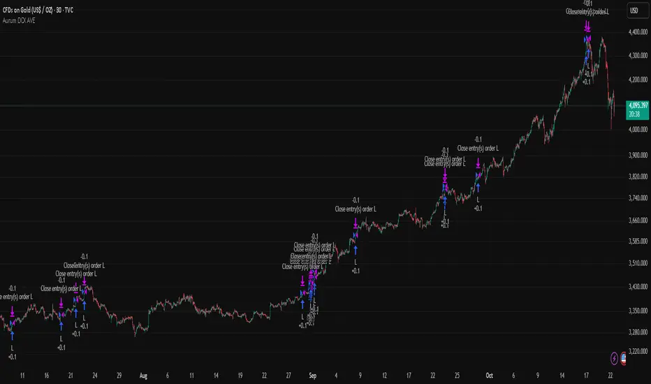
FluxGate Daily Swing StrategySummary in one paragraph
FluxGate treats long and short as different ecosystems. It runs two independent engines so the long side can be bold when the tape rewards upside persistence while the short side can stay selective when downside is messy. The core reads three directional drivers from price geometry then removes overlap before gating with clean path checks. The complementary risk module anchors stop distance to a higher timeframe ATR so a unit means the same thing on SPY and BTC. It can add take profit breakeven and an ATR trail that only activates after the trade earns it. If a stop is hit the strategy can re enter in the same direction on the next bar with a daily retry cap that you control. Add it to a clean chart. Use defaults to see the intended behavior. For conservative workflows evaluate on bar close.
Scope and intent
• Markets. Large cap equities and liquid ETFs major FX pairs US index futures and liquid crypto pairs
• Timeframes. From one minute to daily
• Default demo in this publication. SPY on one day timeframe
• Purpose. Reduce false starts without missing sustained trends by fusing independent drivers and suppressing activity when the path is noisy
• Limits. This is a strategy. Orders are simulated on standard candles. Non standard chart types are not supported for execution
Originality and usefulness
• Unique fusion. FluxGate extracts three drivers that look at price from different angles. Direction measures slope of a smoothed guide and scales by realized volatility so a point of slope does not mean a different thing on different symbols. Persistence looks at short sign agreement to reward series of closes that keep direction. Curvature measures the second difference of a local fit to wake up during convex pushes. These three are then orthonormalized so a strong reading in one does not double count through another.
• Gates that matter. Efficiency ratio prefers direct paths over treadmills. Entropy turns up versus down frequency into an information read. Light fractal cohesion punishes wrinkly paths. Together they slow the system in chop and allow it to open up when the path is clean.
• Separate long and short engines. Threshold tilts adapt to the skew of score excursions. That lets long engage earlier when upside distribution supports it and keeps short cautious where downside surprise and venue frictions are common.
• Practical risk behavior. Stops are ATR anchored on a higher timeframe so the unit is portable. Take profit is expressed in R so two R means the same concept across symbols. Breakeven and trailing only activate after a chosen R so early noise does not squeeze a good entry. Re entry after stop lets the system try again without you babysitting the chart.
• Testability. Every major window and the aggression controls live in Inputs. There is no hidden magic number.
Method overview in plain language
Base measures
• Return basis. Natural log of close over prior close for stability and easy aggregation through time. Realized volatility is the standard deviation of returns over a moving window.
• Range basis for risk. ATR computed on a higher timeframe anchor such as day week or month. That anchor is steady across venues and avoids chasing chart specific quirks.
Components
• Directional intensity. Use an EMA of typical price as a guide. Take the day to day slope as raw direction. Divide by realized volatility to get a unit free measure. Soft clip to keep outliers from dominating.
• Persistence. Encode whether each bar closed up or down. Measure short sign agreement so a string of higher closes scores better than a jittery sequence. This favors push continuity without guessing tops or bottoms.
• Curvature. Fit a short linear regression and compute the second difference of the fitted series. Strong curvature flags acceleration that slope alone may miss.
• Efficiency gate. Compare net move to path length over a gate window. Values near one indicate direct paths. Values near zero indicate treadmill behavior.
• Entropy gate. Convert up versus down frequency into a probability of direction. High entropy means coin toss. The gate narrows there.
• Fractal cohesion. A light read of path wrinkliness relative to span. Lower cohesion reduces the urge to act.
• Phase assist. Map price inside a recent channel to a small signed bias that grows with confidence. This helps entries lean toward the right half of the channel without becoming a breakout rule.
• Shock control. Compare short volatility to long volatility. When short term volatility spikes the shock gate temporarily damps activity so the system waits for pressure to normalize.
Fusion rule
• Normalize the three drivers after removing overlap
• Blend with weights that adapt to your aggression input
• Multiply by the gates to respect path quality
• Smooth just enough to avoid jitter while keeping timing responsive
• Compute an adaptive mean and deviation of the score and set separate long and short thresholds with a small tilt informed by skew sign
• The result is one long score and one short score that can cross their thresholds at different times for the same tape which is a feature not a bug
Signal rule
• A long suggestion appears when the long score crosses above its long threshold while all gates are active
• A short suggestion appears when the short score crosses below its short threshold while all gates are active
• If any required gate is missing the state is wait
• When a position is open the status is in long or in short until the complementary risk engine exits or your entry mode closes and flips
Inputs with guidance
Setup Long
• Base length Long. Master window for the long engine. Typical range twenty four to eighty. Raising it improves selectivity and reduces trade count. Lowering it reacts faster but can increase noise
• Aggression Long. Zero to one. Higher values make thresholds more permissive and shorten smoothing
Setup Short
• Base length Short. Master window for the short engine. Typical range twenty eight to ninety six
• Aggression Short. Zero to one. Lower values keep shorts conservative which is often useful on upward drifting symbols
Entries and UI
• Entry mode. Both or Long only or Short only
Complementary risk engine
• Enable risk engine. Turns on bracket exits while keeping your signal logic untouched
• ATR anchor timeframe. Day Week or Month. This sets the structural unit of stop distance
• ATR length. Default fourteen
• Stop multiple. Default one point five times the anchor ATR
• Use take profit. On by default
• Take profit in R. Default two R
• Breakeven trigger in R. Default one R
Usage recipes
Intraday trend focus
• Entry mode Both
• ATR anchor Week
• Aggression Long zero point five Aggression Short zero point three
• Stop multiple one point five Take profit two R
• Expect fewer trades that stick to directional pushes and skip treadmill noise
Intraday mean reversion focus
• Session windows optional if you add them in your copy
• ATR anchor Day
• Lower aggression both sides
• Breakeven later and trailing later so the first bounce has room
• This favors fade entries that still convert into trends when the path stays clean
Swing continuation
• Signal timeframe four hours or one day
• Confirm timeframe one day if you choose to include bias
• ATR anchor Week or Month
• Larger base windows and a steady two R target
• This accepts fewer entries and aims for larger holds
Properties visible in this publication
• Initial capital 25.000
• Base currency USD
• Default order size percent of equity value three - 3% of the total capital
• Pyramiding zero
• Commission zero point zero three percent - 0.03% of total capital
• Slippage five ticks
• Process orders on close off
• Recalculate after order is filled off
• Calc on every tick off
• Bar magnifier off
• Any request security calls use lookahead off everywhere
Realism and responsible publication
• No performance promises. Past results never guarantee future outcomes
• Fills and slippage vary by venue and feed
• Strategies run on standard candles only
• Shapes can update while a bar is forming and settle on close
• Keep risk per trade sensible. Around one percent is typical for study. Above five to ten percent is rarely sustainable
Honest limitations and failure modes
• Sudden news and thin liquidity can break assumptions behind entropy and cohesion reads
• Gap heavy symbols often behave better with a True Range basis for risk than a simple range
• Very quiet regimes can reduce score contrast. Consider longer windows or higher thresholds when markets sleep
• Session windows follow the exchange time of the chart if you add them
• If stop and target can both be inside a single bar this strategy prefers stop first to keep accounting conservative
Open source reuse and credits
• No reused open source beyond public domain building blocks such as ATR EMA and linear regression concepts
Legal
Education and research only. Not investment advice. You are responsible for your decisions. Test on history and in simulation with realistic costs