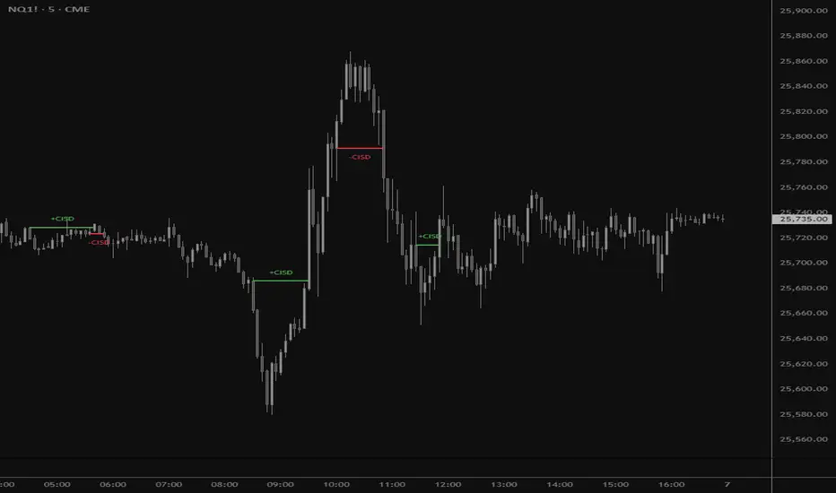
CISD by tncylyvCISD (Change in State of Delivery) by tncylyv
The CISD (Change in State of Delivery) indicator is a precision price action tool designed to help traders identify key reversal points based on ICT concepts. Unlike standard support and resistance indicators, this script tracks the specific algorithmic opening prices responsible for the current delivery state and highlights when that state has been invalidated.
🧠 What is CISD?
Change in State of Delivery refers to the moment price shifts from a Buy Program to a Sell Program (or vice versa).
• Bearish CISD (-CISD): Occurs when price closes below the opening price of the up-candle sequence that created the most recent High.
• Bullish CISD (+CISD): Occurs when price closes above the opening price of the down-candle sequence that created the most recent Low.
This indicator automates the identification of these levels, tracking the "Active" reference price in real-time and marking historical reversals.
🚀 Key Features
1. Continuous Active Level Tracking:
o The indicator plots a continuous, stepped line (The "Active CISD") that follows the market structure. As the market expands (makes new highs or lows), the line updates to the new valid reference point.
o This allows you to see the current invalidation level at a glance without cluttering the chart with old lines.
2. Triggered Reversal Lines:
o When a candle closes beyond the Active CISD level, a "Triggered" line is drawn to mark the exact price and location of the reversal.
o These lines serve as excellent historical references for potential Order Blocks or Breakers later in time.
3. Smart Filtering:
o You can choose to display Both Bullish and Bearish setups, or filter to see Bullish Only or Bearish Only. This is ideal for traders who have a specific daily bias and want to remove noise from the chart.
4. Clean & Customizable:
o Fully customizable colors for Bullish and Bearish events.
o Options to toggle Labels, adjust Line Width, and change Line Styles (Solid, Dashed, Dotted).
o "No Continuation" Logic: This version focuses purely on major reversals (Change in State) rather than minor pullbacks, keeping your chart clean.
⚙️ Settings Guide
• Show Active CISD Level: Toggles the continuous stepped line representing the current threshold for a reversal.
• Triggered CISD Display: Choose between Both, Bullish Only, Bearish Only, or None. This controls the historical lines left behind after a reversal occurs.
• Visual Settings: Adjust line width, label sizes, and font styles to match your chart aesthetic.
• Colors: Customize the Shrek Mode (Bullish) and Blood Bath (Bearish) colors.
⚠️ A Note for Developers
This indicator is open source! If you are a Pine Script developer, feel free to check the source code. I’ve utilized some... creative variable naming conventions to make the coding experience more entertaining. Enjoy the read!
________________________________________
Risk Disclaimer: This tool is for educational purposes and market analysis. It does not guarantee future performance. Always manage your risk.
Indikator dan strategi
Sideways Zone BreakoutSideways Zone Breakout – Advanced Consolidation Breakout Indicator
Created by: Syed Aman Ali
The market spends most of its time moving sideways, trapping traders with false signals and unpredictable whipsaws. This indicator is designed to identify those consolidation phases with precision and highlight confirmed breakout moments where strong momentum is most likely to follow.
🔍 What This Indicator Does
This tool automatically scans recent price action and detects tight sideways zones using a volatility-based measurement. Whenever the market enters a compression phase, the indicator marks the exact upper and lower boundaries of the zone.
Once price closes beyond this range, the indicator instantly triggers a BUY or SELL breakout signal — clean, simple, and highly effective.
🎯 Why This Works
Sideways phases often represent institutional accumulation or distribution. When a breakout occurs, it usually leads to a powerful expansion move. This indicator is specifically built to catch those high-probability moments.
Core logic:
Detects the highest and lowest price within a chosen lookback period
Measures range tightness relative to price
Plots a visual zone only when the market is truly sideways
Generates Buy signals on breakout above the zone
Generates Sell signals on breakdown below the zone
No repainting.
No complex settings.
Pure breakout confirmation based on candle close.
✨ Key Features
✔ Automatic sideways zone detection
✔ Clean upper & lower boundary plotting
✔ Soft shaded zone for visual clarity
✔ Immediate BUY/SELL breakout markers
✔ Alert-ready (great for webhook automation)
✔ Works on all timeframes and all markets
✔ Suitable for crypto, forex, indices, stocks, and commodities
📌 Best Applications
Identifying breakout opportunities after consolidation
Avoiding entries during choppy market conditions
Trend continuation entries after a sideways pause
Scalping volatility expansion
Confirming breakouts with other indicators (EMA / MACD / RSI etc.)
⚡ Important Notes
Breakout signals are confirmed only on candle close, ensuring reliability and zero repainting.
The zone appears only when price is truly consolidating — avoiding unnecessary clutter.
👤 Author
Created by: Syed Aman Ali
Built with a focus on clean charting, market structure, and breakout momentum trading.
If this indicator helps your trading, please leave a like and share your feedback — more high-quality tools are coming soon

HTF Frequency Zone [BigBeluga]🔵 OVERVIEW
HTF Frequency Zone highlights the dominant price level (Point of Control) and the full high–low expansion of any higher timeframe — Daily, Weekly, or Monthly. It captures the frequency of closes inside each HTF candle and plots the most traded “frequency zone”, allowing traders to easily see where price spent the most time and where buy/sell pressure accumulated.
This tool transforms each higher-timeframe bar into a fully visualized structure:
• Top = HTF high
• Bottom = HTF low
• Midline = HTF Frequency POC
• Color-coded zones = bullish or bearish bias
• Labels = counts of bullish and bearish candles inside the HTF range
It is designed to give traders an immediate understanding of high-timeframe balance, imbalance, and price attraction zones.
🔵 CONCEPTS
HTF Partitioning — Each Weekly/Daily/Monthly candle is converted into a dedicated zone with its own High, Low, and Frequency Point of Control.
Frequency POC (Most Touched Price) — The indicator divides the HTF range into 100 bins and counts how many times price closed near each level.
Dominant Zone — The level with the highest frequency becomes the HTF “Value Zone,” plotted as a bold central line.
Directional Bias —
• Bullish HTF zone
• Bearish HTF zone
Internal Candle Counting — Within each HTF period the indicator counts:
• Buy candles (close > open)
• Sell candles (close < open)
This reveals whether intraperiod flow was bullish or bearish.
HTF Structure Blocks — High, Low, and POC are connected across the entire higher-timeframe duration, showing the real shape of HTF balance.
🔵 FEATURES
Automatic HTF Zone Construction — Generates a complete price zone every time the selected timeframe flips (Daily / Weekly / Monthly).
Dynamic High & Low Extraction — The indicator scans every bar inside the HTF window to find true extremes of the range.
100-Level Frequency Scan — Each close within the period is assigned to a bin, creating a detailed distribution of price interaction.
HTF POC Highlighting — The most frequent price level is plotted with a bold red line for immediate visual clarity.
Bull/Bear Coloring —
• Green → Bullish HTF zone.
• Orange → Bearish HTF zone.
Zone Shading — High–Low range is filled with a semi-transparent color matching trend direction.
Buy/Sell Candle Counters — Printed at the top and bottom of each HTF block, showing how many internal candles were bullish or bearish.
POC Label — Displays frequency count (how many touches) at the POC level.
Adaptive Threshold Warning — If bars inside the HTF window are too few (<10), the indicator warns the trader to switch timeframe.
🔵 HOW TO USE
Higher-Timeframe Biasing — Read the zone color to determine if the HTF candle leaned bullish or bearish.
Value Zone Reactions — Price often reacts to the Frequency POC; use it as support/resistance or liquidity magnet.
Range Context — Identify when price is trading near HTF highs (breakout potential) or lows (reversal potential).
Momentum Evaluation — More bullish internal candles = internal buying pressure; more bearish = internal selling pressure.
Swing Trading — Use HTF zones as the “macro map,” then execute trades on lower timeframes aligned with the zone structure.
Liquidity Awareness — The HTF POC often aligns with algorithmic liquidity levels, making it a strong reaction point.
🔵 CONCLUSION
HTF Frequency Zone transforms raw higher-timeframe candles into detailed distribution zones that reveal true market behavior inside the HTF structure. By showing highs, lows, buying/selling activity, and the most interacted price level (Frequency POC), this tool becomes invaluable for traders who want to align executions with powerful HTF levels, liquidity magnets, and structural zones.

ASFX - Automatic VWAPs & Key LevelsAutomate your AVWAPs and key levels for day trading! NY Market open VWAP, Previous day NY VWAP, and more are included. Inital Balance and Opening Range are also automated.

Open Interest RSI [BackQuant]Open Interest RSI
A multi-venue open interest oscillator that aggregates OI across major derivatives exchanges, converts it to coin or USD terms, and runs an RSI-style engine on that aggregated OI so you can track positioning pressure, crowding, and mean reversion in leverage flows, not just in price.
What this is
This tool is an RSI built on top of aggregated open interest instead of price. It pulls futures OI from several major exchanges, converts it into a unified unit (COIN or USD), sums it into a single synthetic OI candle, then applies RSI and smoothing to that combined series.
You can then render that Open Interest RSI in different visual modes:
Clean line or colored line for classic oscillator-style reads.
Column-style oscillator for impulse and compression views.
Flag mode that fills between OI RSI and its EMA for trend/mean reversion blends. See:
Heatmap mode that paints the panel based on OI RSI extremes, ideal for scanning. See:
On top of that it includes:
Aggregated OI source selection (Binance, Bybit, OKX, Bitget, Kraken, HTX, Deribit).
Choice of OI units (COIN or USD).
Reference lines and OB/OS zones.
Extreme highlighting for either trend or mean reversion.
A vertical OI RSI meter that acts as a quick strength gauge.
Aggregated open interest source
Under the hood, the indicator builds a synthetic open interest candle by:
Looping over a list of supported exchanges: Binance, Bybit, OKX, Bitget, Kraken, HTX, Deribit.
Looping over multiple contract suffixes (such as USDT.P, USD.P, USDC.P, USD.PM) to capture different contract types on each venue.
Requesting OI candles from each venue + contract combination for the same underlying symbol.
Converting each OI stream into a common unit: In COIN mode, everything is normalized into coin-denominated OI. In USD mode, coin OI is multiplied by price to approximate notional OI.
Summing up open, high, low and close of OI across venues into a single aggregated OI candle.
If no valid OI is available for the current symbol across all sources, the script throws a clear runtime error so you know you are on an unsupported market.
This gives you a single, exchange-agnostic open interest curve instead of being tied to one venue. That aggregated OI is then passed into the RSI logic.
How the OI RSI is calculated
The RSI side is straightforward, but it is applied to the aggregated OI close:
Compute a base RSI of aggregated OI using the Calculation Period .
Apply a simple moving average of length Smoothing Period (SMA) to reduce noise in the raw OI RSI.
Optionally apply an EMA on top of the smoothed OI RSI as a moving average signal line.
Key parameters:
Calculation Period – base RSI length for OI.
Smoothing Period (SMA) – extra smoothing on the RSI value.
EMA Period – EMA length on the smoothed OI RSI.
The result is:
oi_rsi – raw RSI of aggregated OI.
oi_rsi_s – SMA-smoothed OI RSI.
ma – EMA of the smoothed OI RSI.
Thresholds and extremes
You control three core thresholds:
Mid Point – central reference level, typically 50.
Extreme Upper Threshold – high-level OI RSI edge (for example 80).
Extreme Lower Threshold – low-level OI RSI edge (for example 20).
These thresholds are used for:
Reference lines or OB/OS zone fills.
Heatmap gradient bounds.
Background highlighting of extremes.
The Extreme Highlighting mode controls how extremes are interpreted:
None – do nothing special in extreme regions.
Mean-Rev – background turns red on high OI RSI and green on low OI RSI, framing extremes as contrarian zones.
Trend – background turns green on high OI RSI and red on low OI RSI, framing extremes as participation zones aligned with the prevailing move.
Reference lines and OB/OS zones
You can choose:
None – clean plotting without guides.
Basic Reference Lines – mid, upper and lower thresholds as simple gray horizontals.
OB/OS Levels – filled zones between:
Upper OB: from the upper threshold to 100, colored with the short/overbought color.
Lower OS: from 0 to the lower threshold, colored with the long/oversold color.
These guides help visually anchor the OI RSI within "normal" versus "extreme" regions.
Plotting modes
The Plotting Type input controls how OI RSI is drawn. All modes share the same underlying OI and RSI logic, but emphasise different aspects of the signal.
1) Line mode
This is the classic oscillator representation:
Plots the smoothed OI RSI as a simple line using RSI Line Color and RSI Line Width .
Optionally plots the EMA overlay on the same panel.
Works well when you want standard RSI-style signals on leverage flows: crosses of the midline, divergences versus price, and so on.
2) Colored Line mode
In this mode:
The OI RSI is plotted as a line, but its color is dynamic.
If the smoothed OI RSI is above the mid point, it uses the Long/OB Color .
If it is below the mid point, it uses the Short/OS Color .
This creates an instant visual regime switch between "bullish positioning pressure" and "bearish positioning pressure", while retaining the feel of a traditional RSI line.
3) Oscillator mode
Oscillator mode renders OI RSI as vertical columns around the mid level:
The smoothed OI RSI is plotted as columns using plot.style_columns .
The histogram base is fixed at 50, so bars extend above and below the mid line.
Bar color is dynamic, using long or short colors depending on which side of the mid point the value sits.
This representation makes impulse and compression in OI flows more obvious. It is especially useful when you want to focus on how quickly OI RSI is expanding or contracting around its neutral level. See:
4) Flag mode
Flag mode turns OI RSI and its EMA into a two-line band with a filled area between them:
The smoothed OI RSI and its EMA are both plotted.
A fill is drawn between them.
The fill color flips between the long color and the short color depending on whether OI RSI is above or below its EMA.
Black outlines are added to both lines to make the band clear against any background.
This creates a "flag" style region where:
Green fills show OI RSI leading its EMA, suggesting positive positioning momentum.
Red fills show OI RSI trailing below its EMA, suggesting negative positioning momentum.
Crossovers of the two lines can be read as shifts in OI momentum regime.
Flag mode is useful if you want a more structural view that combines both the level and slope behaviour of OI RSI. See:
5) Heatmap mode
Heatmap mode recasts OI RSI as a single-row gradient instead of a line:
A single row at level 1 is plotted using column style.
The color is pulled from a gradient between the lower and upper thresholds: Near the lower threshold it approaches the short/oversold color and near the upper threshold it approaches the long/overbought color.
The EMA overlay and reference lines are disabled in this mode to keep the panel clean.
This is a very compact way to track OI RSI state at a glance, especially when stacking it alongside other indicators. See:
OI RSI vertical meter
Beyond the main plot, the script can draw a small "thermometer" table showing the current OI RSI position from 0 to 100:
The meter is a two-column table with a configurable number of rows.
Row colors form an inverted gradient: red at the top (100) and green at the bottom (0).
The script clamps OI RSI between 0 and 100 and maps it to a row index.
An arrow marker "▶" is drawn next to the row corresponding to the current OI RSI value.
0 and 100 labels are printed at the ends of the scale for orientation.
You control:
Show OI RSI Meter – turn the meter on or off.
OI RSI Blocks – number of vertical blocks (granularity).
OI RSI Meter Position – panel anchor (top/bottom, left/center/right).
The meter is particularly helpful if you keep the main plot in a small panel but still want an intuitive strength gauge.
How to read it as a market pressure gauge
Because this is an RSI built on aggregated open interest, its extremes and regimes speak to positioning pressure rather than price alone:
High OI RSI (near or above the upper threshold) indicates that open interest has been increasing aggressively relative to its recent history. This often coincides with crowded leverage and a buildup of directional pressure.
Low OI RSI (near or below the lower threshold) indicates aggressive de-leveraging or closing of positions, often associated with flushes, forced unwinds or post-liquidation clean-ups.
Values around the mid point indicate more balanced positioning flows.
You can combine this with price action:
Price up with rising OI RSI suggests fresh leverage joining the move, a more persistent trend.
Price up with falling OI RSI suggests shorts covering or longs taking profit, more fragile upside.
Price down with rising OI RSI suggests aggressive new shorts or levered selling.
Price down with falling OI RSI suggests de-leveraging and potential exhaustion of the move.
Trading applications
Trend confirmation on leverage flows
Use OI RSI to confirm or question a price trend:
In an uptrend, rising OI RSI with values above the mid point indicates supportive leverage flows.
In an uptrend, repeated failures to lift OI RSI above mid point or persistent weakness suggest less committed participation.
In a downtrend, strong OI RSI on the downside points to aggressive shorting.
Mean reversion in positioning
Use thresholds and the Mean-Rev highlight mode:
When OI RSI spends extended time above the upper threshold, the crowd is extended on one side. That can set up squeeze risk in the opposite direction.
When OI RSI has been pinned low, it suggests heavy de-leveraging. Once price stabilises, a re-risking phase is often not far away.
Background colours in Mean-Rev mode help visually identify these periods.
Regime mapping with plotting modes
Different plotting modes give different perspectives:
Heatmap mode for dashboard-style use where you just need to know "hot", "neutral" or "cold" on OI flows at a glance.
Oscillator mode for short term impulses and compression reads around the mid line. See:
Flag mode for blending level and trend of OI RSI into a single banded visual. See:
Settings overview
RSI group
Plotting Type – None, Line, Colored Line, Oscillator, Flag, Heatmap.
Calculation Period – base RSI length for OI.
Smoothing Period (SMA) – smoothing on RSI.
Moving Average group
Show EMA – toggle EMA overlay (not used in heatmap).
EMA Period – length of EMA on OI RSI.
EMA Color – colour of EMA line.
Thresholds group
Mid Point – central reference.
Extreme Upper Threshold and Extreme Lower Threshold – OB/OS thresholds.
Select Reference Lines – none, basic lines or OB/OS zone fills.
Extreme Highlighting – None, Mean-Rev, Trend.
Extra Plotting and UI
RSI Line Color and RSI Line Width .
Long/OB Color and Short/OS Color .
Show OI RSI Meter , OI RSI Blocks , OI RSI Meter Position .
Open Interest Source
OI Units – COIN or USD.
Exchange toggles: Binance, Bybit, OKX, Bitget, Kraken, HTX, Deribit.
Notes
This is a positioning and pressure tool, not a complete system. It:
Models aggregated futures open interest across multiple centralized exchanges.
Transforms that OI into an RSI-style oscillator for better comparability across regimes.
Offers several visual modes to match different workflows, from detailed analysis to compact dashboards.
Use it to understand how leverage and positioning are evolving behind the price, to gauge when the crowd is stretched, and to decide whether to lean with or against that pressure. Attach it to your existing signals, not in place of them.
Also, please check out @NoveltyTrade for the OI Aggregation logic & pulling the data source!
Here is the original script:

RSI For Loop
RSI For Loop – Enhanced RSI Dominance Oscillator
Original concept & innovation ©@viResearch
Enhanced version with historical-comparison loop, median-based statistical strength bands, asymmetric thresholds, and visual upgrades
Core Concept (viResearch)
viResearch was the first to introduce the groundbreaking idea of replacing traditional fixed RSI levels with a loop-based scoring system that evaluates RSI behavior across a defined range, creating a dynamic, self-normalizing momentum score that dramatically reduces false signals in trending markets.
Key Enhancements in This Version
I kept the core brilliance of viResearch's loop concept but completely rewrote the scoring mechanism to make it even more powerful and adaptive:
1. Historical Dominance Comparison
The loop directly compares the current RSI value to the actual RSI values of the previous 1–99 bars (user-adjustable).
→ +1 for every past bar the current RSI beats
→ –1 for every past bar it loses to
This transforms the indicator into a true RSI Dominance / Percentile-Rank oscillator that instantly shows whether current momentum is stronger or weaker than nearly all recent history – perfectly adaptive to any market regime, volatility level, or asset.
2. Median + 3σ Statistical Strength Bands
Added a rolling median of the dominance score plus dynamic ±3σ bands calculated from the RSI score median standard deviation.
These bands identify genuinely extreme momentum phases (statistically rare events) that only occur during the strongest momentum or capitulation moves – giving high-conviction confirmation.
3. Visual & Practical Upgrades
- Clean bar/candle coloring
- On-chart triangle signals at trend changes
- Diamond stepline ±3σ bands
- Built-in alerts for both trend changes and extreme strength phases
- 9 professional color themes
How to Use It
Primary Trend Signals
- Green triangle + bullish bar color → New bullish momentum regime (score crosses above +15)
- Magenta triangle + bearish bar color → New bearish momentum regime (score crosses below –28)
These are some of the cleanest trend-change signals you will ever see – especially powerful on daily/weekly charts.
Extreme Strength Confirmation
Score breaks above the upper 3σ diamond line → Exceptional bullish strength/dominance (add to longs, strength behind the asset)
Score breaks below the lower 3σ diamond line → Exceptional bearish strength/dominance (capitulation or weakness)
These are rarer, very high-probability zones.
Zero-Line Context
Above zero = current RSI stronger than average recent history
Below zero = weaker than average recent history
Near zero = choppy/range-bound (stay out or mean-reversion trade)
Recommended Settings
RSI Length: 46
Loop range: 1 to 99 (~3–6 months on daily)
Long Threshold: +15
Short Threshold: –28
Median Length: 225
SD Length: 60
Works on all assets and timeframes. Absolutely deadly on daily/weekly for swing and position trading, and still excellent on 4H/30min for crypto/stocks.
This enhanced version honors viResearch's original genius while improving on it with true historical comparison and statistical extreme detection – delivering what is, in my opinion, one of the cleanest and most powerful momentum/trend indicators available on TradingView.
Backtests are based on past results and are not indicative of future performance.

Trend Gazer: Unified ICT Trading System with Signals# Trend Gazer User Guide (English)
## 📖 Table of Contents
1. (#about-this-indicator)
2. (#quick-start-guide-3-steps)
3. (#detailed-usage)
4. (#settings-customization)
5. (#why-combine-multiple-features)
6. (#faq)
---
## About This Indicator
**Trend Gazer** is an integrated trading system designed to read institutional order flow like professional traders.
### 🎯 3 Problems This Indicator Solves
#### ❌ Problem 1: Too Many Indicators = Information Overload
```
Normal: RSI + MACD + Moving Average + Bollinger Bands... → Cluttered chart
Solution: All integrated into ONE indicator → Clean & Clear
```
#### ❌ Problem 2: Single Indicators Give False Signals
```
Normal: Enter based on RSI alone → Frequent stop-outs
Solution: Structure × Zone × Momentum multi-angle confirmation → Higher win rate
```
#### ❌ Problem 3: Unclear Entry Timing
```
Normal: Know the trend but don't know WHERE to enter
Solution: LS Bounce Signal shows EXACT entry points
```
---
## Quick Start Guide (3 Steps)
### 🚀 STEP 1: Confirm Trend Direction
**Look for CHoCH (Change of Character)**
```
📍 (1.CHoCH) label = Uptrend starting
📍 (a.CHoCH) label = Downtrend starting
```
**Important**: Wait for CHoCH! No direction without it.
---
### 🎯 STEP 2: Find Entry Points
**Wait for LS Bounce Signal (green/red labels)**
```
🟢 "Long@ HL only" label → LONG (buy) candidate
🔴 "Short@ LH only" label → SHORT (sell) candidate
```
**Label text color meaning**:
- **White text**: Clean trend (high confidence)
- **Yellow text**: Trend transition (moderate caution)
---
### 🛡️ STEP 3: Final Confirmation with Bar Color
**Bar color shows market state**
```
🔴 Red bar: BUY zone (buying is favored)
🟢 Green bar: SELL zone (selling is favored)
⚪ White bar: Neutral (wait and see)
```
---
## Detailed Usage
### 📊 Understanding the Chart
#### 1. Labels (Market Structure Changes)
```
(1.CHoCH) / (a.CHoCH) : Trend reversal
(2.SiMS) / (b.SiMS) : Momentum confirmation
(3.BoMS) / (c.BoMS) : Trend continuation
```
#### 2. Boxes (Institutional Order Zones)
```
📦 Blue boxes: Bullish OB (buy orders accumulated)
📦 Red boxes: Bearish OB (sell orders accumulated)
📦 Black transparent boxes: Liquidity Sweep
```
**How to use Order Blocks**:
- Function as support/resistance
- Signals within OB have higher reliability
- Use for stop-loss placement
#### 3. Lines (Trends and Support/Resistance)
```
━━━ Red lines: EMA20, EMA50, EMA100 (short to mid-term trends)
━━━ Blue lines: 60min NPR/BB bands (support/resistance)
```
#### 4. Bar Colors (Filter 6)
```
Bar color = Real-time market state
🔴 Red: Buying is favored
🟢 Green: Selling is favored
⚪ White: Neutral
```
---
### 🎯 Practical Trading Flow
#### 📍 Preparation Phase
```
1. Open chart (recommended: 5min or 15min)
2. Add Trend Gazer to chart
3. Start in observation mode (don't enter yet)
```
#### 📍 Entry Decision
```
✅ CHoCH confirms direction → Uptrend starting
✅ LS Bounce Signal "Long@ HL only" appears
→ Entry point candidate
✅ Bar turns red → Market supports buying
→ Entry decision 🎯
✅ Place stop below nearest Order Block (blue box)
```
#### 📍 Exit Decision
```
🔴 Opposite LS Bounce Signal "Short@ LH only" appears
→ Consider taking profit
🔴 Bar turns green
→ Potential trend reversal, review position
🔴 Stop loss hit
→ Exit with loss
```
---
### 💡 Tips for Higher Win Rate
#### ✅ DO's
```
1. Enter AFTER CHoCH appears
2. Prioritize white-text LS Bounce Signals
3. Check higher timeframe (1H or Daily) trend
4. Emphasize signals within Order Blocks
5. Use bar color as final confirmation
```
#### ❌ DON'Ts
```
1. Enter before CHoCH → No clear direction
2. Enter only on yellow text → Unstable transition period
3. Ignore bar color → Trading against market state
4. Don't check Order Blocks → Unclear support/resistance
5. Enter same direction consecutively → Overtrading
```
---
## Settings Customization
### 🔧 How to Open Settings
```
1. Right-click on indicator name on chart
2. Select "Settings..."
3. Settings panel opens
```
---
### 📋 Recommended Setting Profiles
#### 🔰 Beginner Settings (Simple)
**Goal**: Reduce noise, show only important signals
```
【FILTERS】
✅ Bonus Filter: ON
✅ Filter 6 (OB/BB/NPR Zone Filter): ON
❌ Direction Filter: OFF
❌ Liquidation Reversal Filter: OFF
❌ ICT Market Structure Filter: OFF
❌ EMA Trend Filter: OFF
❌ OB/FVG Filter 1: OFF
❌ OB/FVG Filter 2: OFF
【SIGNALS】
✅ Signal 0 (Bonus): ON
✅ Signal 1 (VWC Change): ON
✅ Signal 2 (Liq Rev): ON
❌ Signal 3 (LS): OFF (complex alone)
❌ Signal 4 (LS Break): OFF
❌ Signal 5 (OB+LS NPR): OFF
❌ Signal 6 (OB+LS EMA): OFF
【LS BOUNCE SIGNAL】
✅ Exclude EMA50 from touch detection: OFF
❌ Only show when EMA fills are mixed: OFF
```
**What happens with this setup**:
- Only Bonus (black background) signals display
- LS Bounce Signals clearly visible
- Noisy signals filtered out
---
#### 💪 Intermediate Settings (Balanced)
**Goal**: Enable key filters for better accuracy
```
【FILTERS】
✅ Bonus Filter: ON
✅ Filter 6 (OB/BB/NPR Zone Filter): ON
✅ ICT Market Structure Filter: ON
❌ Direction Filter: OFF
❌ Liquidation Reversal Filter: OFF
❌ EMA Trend Filter: OFF
❌ OB/FVG Filter 1: OFF
❌ OB/FVG Filter 2: OFF
【SIGNALS】
✅ Signal 0 (Bonus): ON
✅ Signal 1 (VWC Change): ON
✅ Signal 2 (Liq Rev): ON
✅ Signal 3 (LS): ON
❌ Signal 4 (LS Break): OFF
❌ Signal 5 (OB+LS NPR): OFF
❌ Signal 6 (OB+LS EMA): OFF
【LS BOUNCE SIGNAL】
✅ Exclude EMA50 from touch detection: OFF
❌ Only show when EMA fills are mixed: OFF
```
**What happens with this setup**:
- Signals only after CHoCH (trend confirmed)
- Filter 6 changes bar colors
- Liquidity Sweeps also displayed
---
#### 🚀 Advanced Settings (Full Utilization)
**Goal**: Master all features
```
【FILTERS】
✅ Bonus Filter: ON
✅ Filter 6 (OB/BB/NPR Zone Filter): ON
✅ ICT Market Structure Filter: ON
✅ Direction Filter: ON
✅ EMA Trend Filter: ON
❌ Liquidation Reversal Filter: OFF (optional)
✅ OB/FVG Filter 1: ON
✅ OB/FVG Filter 2: ON
【SIGNALS】
✅ All ON
【LS BOUNCE SIGNAL】
✅ Exclude EMA50 from touch detection: ON (reduce EMA50 noise)
✅ Only show when EMA fills are mixed: ON (show only transition zones)
```
**What happens with this setup**:
- Fewer signals (precision-focused)
- Multiple confirmations greatly reduce false signals
- Only signals confirmed by trend, momentum, and zones
---
### 🎨 Display Customization
#### Change Label Size
```
【BUY/SELL SIGNAL APPEARANCE】
→ "BUY/SELL Label Size"
→ Choose from: tiny / small / normal / large / huge
Recommended: small (default)
```
#### Order Block Display Settings
```
【ORDER BLOCK (OB) SETTINGS】
✅ Show Current TF OB: Current timeframe OB
✅ Show 1min OB: 1-minute OB
✅ Show 5min OB: 5-minute OB
✅ Show 15min OB: 15-minute OB
Recommended: Only 15min OB ON (simple)
```
#### Liquidity Sweep Display
```
【LIQUIDITY SWEEPS SETTINGS】
→ "Sweep Length": Sensitivity (small=frequent, large=selective)
→ "Sweep Option": Standard / Maximum
Recommended: Length=40, Option=Standard
```
#### NPR/BB Bands Display
```
【NPR (NON-REPAINT STDEV) SETTINGS】
✅ Display 60min NPR Bands: 60-minute support/resistance
❌ Display Current TF NPR Bands: Current timeframe (optional)
Recommended: Only 60min ON
```
---
### ⚙️ Advanced Settings
#### Fine-tune Filter 6
```
【FINAL FILTERS】
→ "Enable Filter 6 (OB/BB/NPR Zone Filter)"
When ON:
- Bars color-coded red/green/white
- Behavior at OB, NPR/BB touches controlled
```
#### LS Bounce Signal Adjustments
```
【LS BOUNCE SIGNAL】
→ "Exclude EMA50 from touch detection"
OFF: Detect NPR/BB/EMA50 (all 3)
ON: Detect NPR/BB only (exclude EMA50)
→ "Only show when EMA fills are mixed"
OFF: Show all LS Bounce Signals
ON: Show only transition zone signals (yellow text)
```
#### MTF (Multi-Timeframe) Control
```
【ORDER BLOCK (OB) SETTINGS】
→ "Disable MTF on 1hr+ Charts"
ON: Disable MTF on 1H+ (save memory)
OFF: MTF enabled on all timeframes
Recommended: ON (unnecessary on larger timeframes)
```
---
### 🎯 Purpose-Based Configuration Guide
#### 🔍 Goal 1: Reduce Signal Count
```
✅ Bonus Filter: ON
✅ ICT Market Structure Filter: ON
✅ Filter 6: ON
✅ All Signals OFF, only Signal 0 ON
```
#### 🔍 Goal 2: Get More Signals
```
❌ All Filters OFF
✅ All Signals ON
```
#### 🔍 Goal 3: Trend Following Only
```
✅ ICT Market Structure Filter: ON
✅ Direction Filter: ON
✅ EMA Trend Filter: ON
```
#### 🔍 Goal 4: Counter-Trend Trading
```
✅ LS Bounce Signal: ON
✅ Filter 6: ON
❌ ICT Market Structure Filter: OFF
```
#### 🔍 Goal 5: Day Trading (5-15min charts)
```
✅ Show 15min OB: ON
✅ Display 60min NPR Bands: ON
✅ LS Bounce Signal: ON
❌ Show 1min/5min OB: OFF
```
#### 🔍 Goal 6: Scalping (1-5min charts)
```
✅ Show 5min OB: ON
✅ Show 15min OB: ON
✅ Display 60min NPR Bands: ON
✅ All Signals: ON
```
---
### 💾 Saving and Loading Settings
#### Save Settings
```
1. Click "..." in top-right of Settings screen
2. Select "Save as default"
→ Same settings auto-applied next time
```
#### Reset Settings
```
1. Click "..." in top-right of Settings screen
2. Select "Reset settings"
→ Return to default settings
```
---
## Why Combine Multiple Features?
### 🎯 Problem: Single Indicator Limitations
Common trader problems:
```
❌ RSI alone → Trade against trend, lose
❌ Moving Average alone → Late entry timing
❌ Support/Resistance alone → Caught by false breakouts
```
**Markets are complex**. One angle isn't enough.
---
### 💡 Solution: Multi-Angle Integrated Approach
#### 1️⃣ Structure × Zone × Momentum
```
📐 Structure (ICT CHoCH)
→ "Which direction is likely?"
📦 Zone (OB/NPR/BB)
→ "Where will price react?"
💨 Momentum (EMA/VWC)
→ "Is there momentum now?"
```
**When all 3 align = Highest win-rate timing**
---
#### 2️⃣ Multi-Timeframe Analysis
```
Big picture: Confirm Daily direction
Medium-term: Check 1H Order Blocks
Short-term: Time entry on 5min
```
**Short-term entries aligned with higher timeframes = Better win rate**
---
#### 3️⃣ Understanding Liquidity
```
🎣 Institutional strategy:
1. Intentionally move price opposite to stop out retail
2. Then, move in real direction
💡 Liquidity Sweep = Visualize this "trap"
→ Read institutional order flow
```
---
### 🧠 Integration Examples
#### Case 1: RSI Alone vs Integrated System
**Scenario**: RSI at 30 (oversold)
```
❌ RSI-only decision:
→ "Buy!"
→ But downtrend continues, loss 😢
✅ Trend Gazer:
CHoCH check → Still downtrend ❌
Order Block → In Bearish OB ❌
LS Bounce → SHORT signal only ❌
→ Skip or SHORT
→ Avoid loss ✅
```
**Result**: Multiple filters block wrong entry
---
#### Case 2: LS Bounce Signal 2-Stage Logic
**Scenario**: Price touches 60min NPR lower band
```
🔍 Traditional method:
Touched → Buy!
→ But price continues down 😢
✅ Trend Gazer:
Stage 1: NPR touch + red bar → Flag ON
Stage 2: EMA20 crosses above EMA50 → Confirm bounce
→ Now "Long@ HL only" displays
→ Entry → Success ✅
```
**Result**: Not just "touch" but "touch + bounce confirmation" improves accuracy
---
### 🎓 Progressive Learning Design
This indicator is designed for **beginners to advanced**:
```
📖 Beginner (Month 1):
Use only CHoCH + LS Bounce Signal
→ Learn trend and entry points
📖 Intermediate (Months 2-3):
Add Order Block + Bar Color
→ Learn support/resistance and filtering
📖 Advanced (Month 6+):
Master all features
→ Read institutional order flow
```
**Ultimate goal**: Indicator becomes confirmation tool. Your market sense becomes primary.
---
### 🔬 Technical Advantages
#### 1. Non-Repaint STDEV (NPR)
```
Normal Bollinger Bands:
→ Past data changes (repaints)
→ Inaccurate backtesting
NPR:
→ Past data doesn't change (non-repaint)
→ Reliable verification possible
```
#### 2. 2-Stage Signal Logic
```
Traditional: Condition met → Immediate signal
→ Many false signals
Trend Gazer: Condition1 → Flag ON → Condition2 → Signal
→ Confirmation step improves accuracy
```
#### 3. Alternating Filter
```
Problem: Same-direction signals spam
→ Overtrading
Solution: LONG → SHORT → LONG alternating only
→ Prevent unnecessary entries
```
---
### 💎 Conclusion: Why Integration?
```
Single indicator = "Partial truth"
Integrated system = "3D market perspective"
```
**Markets are multifaceted**. One angle isn't enough.
Trend Gazer **integrates multiple screens pros watch simultaneously into ONE**,
allowing beginners to read charts with institutional perspective.
---
## FAQ
### ❓ Q1: Which timeframe is best?
**A**: Depends on trading style
```
Scalping: 1min ~ 5min
Day Trading: 5min ~ 15min
Swing: 1H ~ 4H
```
**Important**: LS Bounce Signal only works on 30min and below.
---
### ❓ Q2: Too many signals, confused
**A**: Enable filters
```
【Recommended Settings】
✅ Bonus Filter: ON
✅ Filter 6: ON
✅ ICT Market Structure Filter: ON
→ Show only Signal 0
```
This significantly reduces signal count.
---
### ❓ Q3: No CHoCH appearing, what to do?
**A**: Wait or check higher timeframe
```
Method 1: Wait for CHoCH (recommended)
Method 2: Check higher timeframe (e.g., Daily) for trend
Method 3: Disable ICT Filter (not recommended)
```
**When trend is unclear, sitting out is also strategy**.
---
### ❓ Q4: LS Bounce Signal not appearing
**A**: Checkpoints
```
1. Are you on 30min or below chart?
→ Doesn't show on 1H+
2. Are NPR/BB bands displayed?
→ Check Settings "Display 60min NPR Bands"
3. Is EMA50 excluded?
→ If "Exclude EMA50" is ON, EMA50 signals won't show
```
---
### ❓ Q5: Bar color not changing?
**A**: Check Filter 6
```
Settings → FINAL FILTERS
→ Confirm "Enable Filter 6 (OB/BB/NPR Zone Filter)" is ON
If ON but still not changing:
→ Current price may be outside OB/NPR/BB zones
```
---
### ❓ Q6: Too many Order Blocks, hard to see
**A**: Narrow down displayed OBs
```
Settings → ORDER BLOCK (OB) SETTINGS
Recommended:
❌ Show Current TF OB: OFF
❌ Show 1min OB: OFF
❌ Show 5min OB: OFF
✅ Show 15min OB: ON (only this)
```
---
### ❓ Q7: How to improve win rate?
**A**: Thorough multiple confirmations
```
Checklist:
✅ CHoCH appeared
✅ LS Bounce Signal (white text)
✅ Bar color matches (red bar=LONG, green bar=SHORT)
✅ Signal within Order Block
✅ Aligns with higher timeframe trend
Enter ONLY when all align
```
---
### ❓ Q8: Want to practice on demo
**A**: Recommended practice method
```
Week 1: Observation only
→ Watch signals and chart movement
→ Resist entering
Weeks 2-3: Keep records
→ Screenshot when signal appears
→ Record subsequent movement
Week 4+: Start demo trading
→ Start with small amounts
→ Continue keeping records
```
---
### ❓ Q9: Are there alert features?
**A**: Yes, multiple alerts available
```
Setup method:
1. Right-click indicator on chart
2. Select "Add Alert..."
3. Choose from:
- ANY ALERT: BUY/SELL Signals
- BUY ONLY ALERT
- SELL ONLY ALERT
- MS UP / MS DOWN
- BAR COLOR: RED / LIME
- LS BOUNCE: LONG / SHORT Signal
```
---
### ❓ Q10: Works on other markets?
**A**: Yes, works on all markets
```
✅ Cryptocurrency (BTC, ETH, etc.)
✅ Forex (EUR/USD, USD/JPY, etc.)
✅ Stocks (individual stocks, indices)
✅ Futures (oil, gold, etc.)
```
Works on any market with price and volume data.
---
## 📋 Disclaimer
### ⚠️ Important Notice
This indicator is for **educational and informational purposes only**.
```
❌ NOT investment advice
❌ Does NOT guarantee profits
❌ Past results do NOT guarantee future performance
```
### Risk Warning
```
⚠️ Trading involves substantial risk
⚠️ Only trade with funds you can afford to lose
⚠️ Practice extensively on demo account before live trading
⚠️ Make your own informed decisions and act at your own risk
```
---
## 📞 Support
### Feedback & Questions
Feel free to ask questions in TradingView comments section.
### Bug Reports
Please report with specific details (timeframe, symbol, screenshots).
---
**Author**: rasukaru666
**License**: Mozilla Public License 2.0
**Last Updated**: December 2025
**Version**: Latest
---
**Thank you for using Trend Gazer!**
**Happy Trading! 📈**
---------------

FVG Supply and DemandThis indicator combines powerful tools into one:
• Supply & Demand Zones built from swing highs/lows with ATR-based zone width, POI markers, and Break-of-Structure (BOS) detection.
• Volumized Fair Value Gaps (FVGs) showing bullish/bearish gaps, total volume inside the gap, volume distribution, optional zone-combining, and auto-cleanup.
• Swing TSL Line and manage bar color.
It helps visualize key imbalance areas, institutional zones, and price reaction points.
Credits to the Author.
⚠️ Disclaimer
This indicator is provided for educational and analytical purposes only.
It does not provide trading advice.
Past results do not guarantee future outcomes.
Use responsibly and in conjunction with your market analysis.
The Rumer's Box Theory“The Rumer's Box Theory” is a visual trading indicator that allows traders to quickly identify the previous daily candle’s high and low across any timeframe. It displays a purple box spanning the previous day’s high to low, with a blue horizontal line marking the 50% midpoint for quick reference. The settings also provide options to extend the box and midpoint line to the left, giving traders flexibility in how the indicator appears on the chart.

Impulse Reactor RSI-SMA Trend Indicator [ApexLegion]Impulse Reactor RSI-SMA Trend Indicator
Introduction and Theoretical Background
Design Rationale
Standard indicators frequently generate binary 'BUY' or 'SELL' signals without accounting for the broader market context. This often results in erratic "Flip-Flop" behavior, where signals are triggered indiscriminately regardless of the prevailing volatility regime.
Impulse Reactor was engineered to address this limitation by unifying two critical requirements: Quantitative Rigor and Execution Flexibility.
The Solution
Composite Analytical Framework This script is not a simple visual overlay of existing indicators. It is an algorithmic synthesis designed to function as a unified decision-making engine. The primary objective was to implement rigorous quantitative analysis (Volatility Normalization, Structural Filtering) directly within an alert-enabled framework. This architecture is designed to process signals through strict, multi-factor validation protocols before generating real-time notifications, allowing users to focus on structurally validated setups without manual monitoring.
How It Works
This is not a simple visual mashup. It utilizes a cross-validation algorithm where the Trend Structure acts as a gatekeeper for Momentum signals:
Logic over Lag: Unlike simple moving average crossovers, this script uses a 15-layer Gradient Ribbon to detect "Laminar Flow." If the ribbon is knotted (Compression), the system mathematically suppresses all signals.
Volatility Normalization: The core calculation adapts to ATR (Average True Range). This means the indicator automatically expands in volatile markets and contracts in quiet ones, maintaining accuracy without constant manual tweaking.
Adaptive Signal Thresholding: It incorporates an 'Anti-Greed' algorithm (Dynamic Thresholding) that automatically adjusts entry criteria based on trend duration. This logic aims to mitigate the risk of entering positions during periods of statistical trend exhaustion.
Why Use It?
Market State Decoding: The gradient Ribbon visualizes the underlying trend phase in real-time.
◦ Cyan/Blue Flow: Strong Bullish Trend (Laminar Flow).
◦ Magenta/Pink Flow: Strong Bearish Trend.
◦ Compressed/Knotted: When the ribbon lines are tightly squeezed or overlapping, it signals Consolidation. The system filters signals here to avoid chop.
Noise Reduction: The goal is not to catch every pivot, but to isolate high-confidence setups. The logic explicitly filters out minor fluctuations to help maintain position alignment with the broader trend.
⚖️ Chapter 1: System Architecture
Introduction: Composite Analytical Framework
System Overview
Impulse Reactor serves as a comprehensive technical analysis engine designed to synthesize three distinct market dimensions—Momentum, Volatility, and Trend Structure—into a unified decision-making framework. Unlike traditional methods that analyze these metrics in isolation, this system functions as a central processing unit that integrates disparate data streams to construct a coherent model of market behavior.
Operational Objective
The primary objective is to transition from single-dimensional signal generation to a multi-factor assessment model. By fusing data from the Impulse Core (Volatility), Gradient Oscillator (Momentum), and Structural Baseline (Trend), the system aims to filter out stochastic noise and identify high-probability trade setups grounded in quantitative confluence.
Market Microstructure Analysis: Limitations of Conventional Models
Extensive backtesting and quantitative analysis have identified three critical inefficiencies in standard oscillator-based strategies:
• Bounded Oscillator Limitations (The "Oscillation Trap"): Traditional indicators such as RSI or Stochastics are mathematically constrained between fixed values (0 to 100). In strong trending environments, these metrics often saturate in "overbought" or "oversold" zones. Consequently, traders relying on static thresholds frequently exit structurally valid positions prematurely or initiate counter-trend trades against prevailing momentum, resulting in suboptimal performance.
• Quantitative Blindness to Quality: Standard moving averages and trend indicators often fail to distinguish the qualitative nature of price movement. They treat low-volume drift and high-velocity expansion identically. This inability to account for "Volatility Quality" leads to delayed responsiveness during critical market events.
• Fractal Dissonance (Timeframe Disconnect): Financial markets exhibit fractal characteristics where trends on lower timeframes may contradict higher timeframe structures. Manual integration of multi-timeframe analysis increases cognitive load and susceptibility to human error, often resulting in conflicting biases at the point of execution.
Core Design Principles
To mitigate the aforementioned systemic inefficiencies, Impulse Reactor employs a modular architecture governed by three foundational principles:
Principle A:
Volatility Precursor Analysis Market mechanics demonstrate that volatility expansion often functions as a leading indicator for directional price movement. The system is engineered to detect "Volatility Deviation" — specifically, the divergence between short-term and long-term volatility baselines—prior to its manifestation in price action. This allows for entry timing aligned with the expansion phase of market volatility.
Principle B:
Momentum Density Visualization The system replaces singular momentum lines with a "Momentum Density" model utilizing a 15-layer Simple Moving Average (SMA) Ribbon.
• Concept: This visualization represents the aggregate strength and consistency of the trend.
• Application: A fully aligned and expanded ribbon indicates a robust trend structure ("Laminar Flow") capable of withstanding minor counter-trend noise, whereas a compressed ribbon signals consolidation or structural weakness.
Principle C:
Adaptive Confluence Protocols Signal validity is strictly governed by a multi-dimensional confluence logic. The system suppresses signal generation unless there is synchronized confirmation across all three analytical vectors:
1. Volatility: Confirmed expansion via the Impulse Core.
2. Momentum: Directional alignment via the Hybrid Oscillator.
3. Structure: Trend validation via the Baseline. This strict filtering mechanism significantly reduces false positives in non-trending (choppy) environments while maintaining sensitivity to genuine breakouts.
🔍 Chapter 2: Core Modules & Algorithmic Logic
Module A: Impulse Core (Normalized Volatility Deviation)
Operational Logic The Impulse Core functions as a volatility-normalized momentum gauge rather than a standard oscillator. It is designed to identify "Volatility Contraction" (Squeeze) and "Volatility Expansion" phases by quantifying the divergence between short-term and long-term volatility states.
Volatility Z-Score Normalization
The formula implements a custom normalization algorithm. Unlike standard oscillators that rely on absolute price changes, this logic calculates the Z-Score of the Volatility Spread.
◦ Numerator: (atr_f - atr_s) captures the raw momentum of volatility expansion.
◦ Denominator: (std_f + 1e-6) standardizes this value against historical variance.
◦ Result: This allows the indicator scales consistently across assets (e.g., Bitcoin vs. Euro) without manual recalibration.
f_impulse() =>
atr_f = ta.atr(fastLen) // Fast Volatility Baseline
atr_s = ta.atr(slowLen) // Slow Volatility Baseline
std_f = ta.stdev(atr_f, devLen) // Volatility Standard Deviation
(atr_f - atr_s) / (std_f + 1e-6) // Normalized Differential Calculation
Algorithmic Framework
• Differential Calculation: The system computes the spread between a Fast Volatility Baseline (ATR-10) and a Slow Volatility Baseline (ATR-30).
• Normalization Protocol: To standardize consistency across diverse asset classes (e.g., Forex vs. Crypto), the raw differential is divided by the standard deviation of the volatility itself over a 30-period lookback.
• Signal Generation:
◦ Contraction (Squeeze): When the Fast ATR compresses below the Slow ATR, it registers a potential volatility buildup phase.
◦ Expansion (Release): A rapid divergence of the Fast ATR above the Slow ATR signals a confirmed volatility expansion, validating the strength of the move.
Module B: Gradient Oscillator (RSI-SMA Hybrid)
Design Rationale To mitigate the "noise" and "false reversal" signals common in single-line oscillators (like standard RSI), this module utilizes a 15-Layer Gradient Ribbon to visualize momentum density and persistence.
Technical Architecture
• Ribbon Array: The system generates 15 sequential Simple Moving Averages (SMA) applied to a volatility-adjusted RSI source. The length of each layer increases incrementally.
• State Analysis:
Momentum Alignment (Laminar Flow): When all 15 layers are expanded and parallel, it indicates a robust trend where buying/selling pressure is distributed evenly across multiple timeframes. This state helps filter out premature "overbought/oversold" signals.
• Consolidation (Compression): When the distance between the fastest layer (Layer 1) and the slowest layer (Layer 15) approaches zero or the layers intersect, the system identifies a "Non-Tradable Zone," preventing entries during choppy market conditions.
// Laminar Flow Validation
f_validate_trend() =>
// Calculate spread between Ribbon layers
ribbon_spread = ta.stdev(ribbon_array, 15)
// Only allow signals if Ribbon is expanded (Laminar Flow)
is_flowing = ribbon_spread > min_expansion_threshold
// If compressed (Knotted), force signal to false
is_flowing ? signal : na
Module C: Adaptive Signal Filtering (Behavioral Bias Mitigation)
This subsystem, operating as an algorithmic "Anti-Greed" Mechanism, addresses the statistical tendency for signal degradation following prolonged trends.
Dynamic Threshold Adjustment
• Win Streak Detection: The algorithm internally tracks the outcome of closed trade cycles.
• Sensitivity Multiplier: Upon detecting consecutive successful signals in the same direction, a Penalty_Factor is applied to the entry logic.
• Operational Impact: This effectively raises the Required_Slope threshold for subsequent signals. For example, after three consecutive bullish signals, the system requires a 30% steeper trend angle to validate a fourth entry. This enforces stricter discipline during extended trends to reduce the probability of entering at the point of trend exhaustion.
Anti-Greed Logic: Dynamic Threshold Calculation
f_adjust_threshold(base_slope, win_streak) =>
// Adds a 10% penalty to the difficulty for every consecutive win
penalty_factor = 0.10
risk_scaler = 1 + (win_streak * penalty_factor)
// Returns the new, harder-to-reach threshold
base_slope * risk_scaler
Module D: Trend Baseline (Triple-Smoothed Structure)
The Trend Baseline serves as the structural filter for all signals. It employs a Triple-Smoothed Hybrid Algorithm designed to balance lag reduction with noise filtration.
Smoothing Stages
1. Volatility Banding: Utilizes a SuperTrend-based calculation to establish the upper and lower boundaries of price action.
2. Weighted Filter: Applies a Weighted Moving Average (WMA) to prioritize recent price data.
3. Exponential Smoothing: A final Exponential Moving Average (EMA) pass is applied to create a seamless baseline curve.
Functionality
This "Heavy" baseline resists minor intraday volatility spikes while remaining responsive to sustained structural shifts. A signal is only considered valid if the price action maintains structural integrity relative to this baseline
🚦 Chapter 3: Risk Management & Exit Protocols
Quantitative Risk Management (TP/SL & Trailing)
Foundational Architecture: Volatility-Adjusted Geometry Unlike strategies relying on static nominal values, Impulse Reactor establishes dynamic risk boundaries derived from quantitative volatility metrics. This design aligns trade invalidation levels mathematically with the current market regime.
• ATR-Based Dynamic Bracketing:
The protocol calculates Stop-Loss and Take-Profit levels by applying Fibonacci coefficients (Default: 0.786 for SL / 1.618 for TP) to the Average True Range (ATR).
◦ High Volatility Environments: The risk bands automatically expand to accommodate wider variance, preventing premature exits caused by standard market noise.
◦ Low Volatility Environments: The bands contract to tighten risk parameters, thereby dynamically adjusting the Risk-to-Reward (R:R) geometry.
• Close-Validation Protocol ("Soft Stop"):
Institutional algorithms frequently execute liquidity sweeps—driving prices briefly below key support levels to accumulate inventory.
◦ Mechanism: When the "Soft Stop" feature is enabled, the system filters out intraday volatility spikes. The stop-loss is conditional; execution is triggered only if the candle closes beyond the invalidation threshold.
◦ Strategic Advantage: This logic distinguishes between momentary price wicks and genuine structural breakdowns, preserving positions during transient volatility.
• Step-Function Trailing Mechanism:
To protect unrealized PnL while allowing for normal price breathing, a two-phase trailing methodology is employed:
◦ Phase 1 (Activation): The trailing function remains dormant until the price advances by a pre-defined percentage threshold.
◦ Phase 2 (Dynamic Floor): Once armed, the stop level creates a moving floor, adjusting relative to price action while maintaining a volatility-based (ATR) buffer to systematically protect unrealized PnL.
• Algorithmic Exit Protocols (Dynamic Liquidity Analysis)
◦ Rationale: Inefficiencies of Static Targets Static "Take Profit" levels often result in suboptimal exits. They compel traders to close positions based on arbitrary figures rather than evolving market structure, potentially capping upside during significant trends or retaining positions while the underlying trend structure deteriorates.
◦ Solution: Structural Integrity Assessment The system utilizes a Dynamic Liquidity Engine to continuously audit the validity of the position. Instead of targeting a specific price point, the algorithm evaluates whether the trend remains statistically robust.
Multi-Factor Exit Logic (The Tri-Vector System)
The Smart Exit protocol executes only when specific algorithmic invalidation criteria are met:
• 1. Momentum Exhaustion (Confluence Decay): The system monitors a 168-hour rolling average of the Confluence Score. A significant deviation below this historical baseline indicates momentum exhaustion, signaling that the driving force behind the trend has dissipated prior to a price reversal. This enables preemptive exits before a potential drawdown.
• 2. Statistical Over-Extension (Mean Reversion): Utilizing the core volatility logic, the system identifies instances where price deviates beyond 2.0 standard deviations from the mean. While the trend may be technically bullish, this statistical anomaly suggests a high probability of mean reversion (elastic snap-back), triggering a defensive exit to capitalize on peak valuation.
• 3. Oscillator Rejection (Immediate Pivot): To manage sudden V-shaped volatility, the system monitors RSI pivots. If a sharp "Pivot High" or divergence is detected, the protocol triggers an immediate "Peak Exit," bypassing standard trend filters to secure liquidity during high-velocity reversals.
🎨 Chapter 4: Visualization Guide
Gradient Oscillator Ribbon
The 15-layer SMA ribbon visualized via plot(r1...r15) represents the "Momentum Density" of the market.
• Visuals:
◦ Cyan/Blue Ribbon: Indicates Bullish Momentum.
◦ Pink/Magenta Ribbon: Indicates Bearish Momentum.
• Interpretation:
◦ Laminar Flow: When the ribbon expands widely and flows in parallel, it signifies a robust trend where momentum is distributed evenly across timeframes. This is the ideal state for trend-following.
◦ Compression (Consolidation): If the ribbon becomes narrow, twisted, or knotted, it indicates a "Non-Tradable Zone" where the market lacks a unified direction. Traders are advised to wait for clarity.
◦ Over-Extension: If the top layer crosses the Overbought (85) or Oversold (15) lines, it visually warns of potential market overheating.
Trend Baseline
The thick, color-changing line plotted via plot(baseline) represents the Structural Backbone of the market.
• Visuals: Changes color based on the trend direction (Blue for Bullish, Pink for Bearish).
• Interpretation:
Structural Filter: Long positions are statistically favored only when price action sustains above this baseline, while short positions are favored below it.
Dynamic Support/Resistance: The baseline acts as a dynamic support level during uptrends and resistance during downtrends.
Entry Signals & Labels
Text labels ("Long Entry", "Short Entry") appear when the system detects high-probability setups grounded in quantitative confluence.
• Visuals: Labeled signals appear above/below specific candles.
• Interpretation:
These signals represent moments where Volatility (Expansion), Momentum (Alignment), and Structure (Trend) are synchronized.
Smart Exit: Labels such as "Smart Exit" or "Peak Exit" appear when the system detects momentum exhaustion or structural decay, prompting a defensive exit to preserve capital.
Dynamic TP/SL Boxes
The semi-transparent colored zones drawn via fill() represent the risk management geometry.
• Visuals: Colored boxes extending from the entry point to the Take Profit (TP) and Stop Loss (SL) levels.
• Function:
Volatility-Adjusted Geometry: Unlike static price targets, these boxes expand during high volatility (to prevent wicks from stopping you out) and contract during low volatility (to optimize Risk-to-Reward ratios).
SAR + MACD Glow
Small glowing shapes appearing above or below candles.
• Visuals: Triangle or circle glows near the price bars.
• Interpretation:
This visual indicates a secondary confirmation where Parabolic SAR and MACD align with the main trend direction. It serves as an additional confluence factor to increase confidence in the trade setup.
Support/Resistance Table
A small table located at the bottom-right of the chart.
• Function: Automatically identifies and displays recent Pivot Highs (Resistance) and Pivot Lows (Support).
• Interpretation: These levels can be used as potential targets for Take Profit or invalidation points for manual Stop Loss adjustments.
🖥️ Chapter 5: Dashboard & Operational Guide
Integrated Analytics Panel (Dashboard Overview)
To facilitate rapid decision-making without manual calculation, the system aggregates critical market dimensions into a unified "Heads-Up Display" (HUD). This panel monitors real-time metrics across multiple timeframes and analytical vectors.
A. Intermediate Structure (12H Trend)
• Function: Anchors the intraday analysis to the broader market structure using a 12-hour rolling window.
• Interpretation:
◦ Bullish (> +0.5%): Indicates a positive structural bias. Long setups align with the macro flow.
◦ Bearish (< -0.5%): Indicates structural weakness. Short setups are statistically favored.
◦ Neutral: Represents a ranging environment where the Confluence Score becomes the primary weighting factor.
B. Composite Confluence Score (Signal Confidence)
• Definition: A probability metric derived from the synchronization of Volatility (Impulse Core), Momentum (Ribbon), and Trend (Baseline).
• Grading Scale:
Strong Buy/Sell (> 7.0 / < 3.0): Indicates full alignment across all three vectors. Represents a "Prime Setup" eligible for standard position sizing.
Buy/Sell (5.0–7.0 / 3.0–5.0): Indicates a valid trend but with moderate volatility confirmation.
Neutral: Signals conflicting data (e.g., Bullish Momentum vs. Bearish Structure). Trading is not recommended ("No-Trade Zone").
C. Statistical Deviation Status (Mean Reversion)
• Logic: Utilizes Bollinger Band deviation principles to quantify how far price has stretched from the statistical mean (20 SMA).
• Alert States:
Over-Extended (> 2.0 SD): Warning that price is statistically likely to revert to the mean (Elastic Snap-back), even if the trend remains technically valid. New entries are discouraged in this zone.
Normal: Price is within standard distribution limits, suitable for trend-following entries.
D. Volatility Regime Classification
• Metric: Compares current ATR against a 100-period historical baseline to categorize the market state.
• Regimes:
Low Volatility (Lvl < 1.0): Market Compression. Often precedes volatility expansion events.
Mid Volatility (Lvl 1.0 - 1.5): Standard operating environment.
High Volatility (Lvl > 1.5): Elevated market stress. Risk parameters should be adjusted (e.g., reduced position size) to account for increased variance.
E. Performance Telemetry
• Function: Displays the historical reliability of the Trend Baseline for the current asset and timeframe.
• Operational Threshold: If the displayed Win Rate falls below 40%, it suggests the current market behavior is incoherent (choppy) and does not respect trend logic. In such cases, switching assets or timeframes is recommended.
Operational Protocols & Signal Decoding
Visual Interpretation Standards
• Laminar Flow (Trade Confirmation): A valid trend is visually confirmed when the 15-layer SMA Ribbon is fully expanded and parallel. This indicates distributed momentum across timeframes.
• Consolidation (No-Trade): If the ribbon appears twisted, knotted, or compressed, the market lacks a unified directional vector.
• Baseline Interaction: The Triple-Smoothed Baseline acts as a dynamic support/resistance filter. Long positions remain valid only while price sustains above this structure.
System Calibration (Settings)
• Adaptive Signal Filtering (Prev. Anti-Greed): Enabled by default. This logic automatically raises the required trend slope threshold following consecutive wins to mitigate behavioral bias.
• Impulse Sensitivity: Controls the reactivity of the Volatility Core. Higher settings capture faster moves but may introduce more noise.
⚙️ Chapter 6: System Configuration & Alert Guide
This section provides a complete breakdown of every adjustable setting within Impulse Reactor to assist you in tailoring the engine to your specific needs.
🌐 LANGUAGE SETTINGS (Localization)
◦ Select Language (Default: English):
Function: Instantly translates all chart labels, dashboard texts into your preferred language.
Supported: English, Korean, Chinese, Spanish
⚡ IMPULSE CORE SETTINGS (Volatility Engine)
◦ Deviation Lookback (Default: 30): The period used to calculate the standard deviation of volatility.
Role: Sets the baseline for normalizing momentum. Higher values make the core smoother but slower to react.
◦ Fast Pulse Length (Default: 10): The short-term ATR period.
Role: Detects rapid volatility expansion.
◦ Slow Pulse Length (Default: 30): The long-term ATR baseline.
Role: Establishes the background volatility level. The core signal is derived from the divergence between Fast and Slow pulses.
🎯 TP/SL SETTINGS (Risk Management)
◦ SL/TP Fibonacci (Default: 0.786 / 1.618): Selects the Fibonacci ratio used for risk calculation.
◦ SL/TP Multiplier (Default: 1.5 / 2): Applies a multiplier to the ATR-based bands.
Role: Expands or contracts the Take Profit and Stop Loss boxes. Increase these values for higher volatility assets (like Altcoins) to avoid premature stop-outs.
◦ ATR Length (Default: 14): The lookback period for calculating the Average True Range used in risk geometry.
◦ Use Soft Stop (Close Basis):
Role: If enabled, Stop Loss alerts only trigger if a candle closes beyond the invalidation level. This prevents being stopped out by wick manipulations.
🔊 RIBBON SETTINGS (Momentum Visualization)
◦ Show SMA Ribbon: Toggles the visibility of the 15-layer gradient ribbon.
◦ Ribbon Line Count (Default: 15): The number of SMA lines in the ribbon array.
◦ Ribbon Start Length (Default: 2) & Step (Default: 1): Defines the spread of the ribbon.
Role: Controls the "thickness" of the momentum density visualization. A wider step creates a broader ribbon, useful for higher timeframes.
📎 DISPLAY OPTIONS
◦ Show Entry Lines / TP/SL Box / Position Labels / S/R Levels / Dashboard: Toggles individual visual elements on the chart to reduce clutter.
◦ Show SAR+MACD Glow: Enables the secondary confirmation shapes (triangles/circles) above/below candles.
📈 TREND BASELINE (Structural Filter)
◦ Supertrend Factor (Default: 12) & ATR Period (Default: 90): Controls the sensitivity of the underlying Supertrend algorithm used for the baseline calculation.
◦ WMA Length (40) & EMA Length (14): The smoothing periods for the Triple-Smoothed Baseline.
◦ Min Trend Duration (Default: 10): The minimum number of bars the trend must be established before a signal is considered valid.
🧠 SMART EXIT (Dynamic Liquidity)
◦ Use Smart Exit: Enables the momentum exhaustion logic.
◦ Exit Threshold Score (Default: 3): The sensitivity level for triggering a Smart Exit. Lower values trigger earlier exits.
◦ Average Period (168) & Min Hold Bars (5): Defines the rolling window for momentum decay analysis and the minimum duration a trade must be held before Smart Exit logic activates.
🛡️ TRAILING STOP (Step)
◦ Use Trailing Stop: Activates the step-function trailing mechanism.
◦ Step 1 Activation % (0.5) & Offset % (0.5): The price must move 0.5% in your favor to arm the first trail level, which sets a stop 0.5% behind price.
◦ Step 2 Activation % (1) & Offset % (0.2): Once price moves 1%, the trail tightens to 0.2%, securing the position.
🌀 SAR & MACD SETTINGS (Secondary Confirmation)
◦ SAR Start/Increment/Max: Standard Parabolic SAR parameters.
◦ SAR Score Scaling (ATR): Adjusts how much weight the SAR signal has in the overall confluence score.
◦ MACD Fast/Slow/Signal: Standard MACD parameters used for the "Glow" signals.
🔄 ANTI-GREED LOGIC (Behavioral Bias)
◦ Strict Entry after Win: Enables the negative feedback loop.
◦ Strict Multiplier (Default: 1.1): Increases the entry difficulty by 10% after each win.
Role: Prevents overtrading and entering at the top of an extended trend.
🌍 HTF FILTER (Multi-Timeframe)
◦ Use Auto-Adaptive HTF Filter: Automatically selects a higher timeframe (e.g., 1H -> 4H) to filter signals.
◦ Bypass HTF on Steep Trigger: Allows an entry even against the HTF trend if the local momentum slope is exceptionally steep (catch powerful reversals).
📉 RSI PEAK & CHOPPINESS
◦ RSI Peak Exit (Instant): Triggers an immediate exit if a sharp RSI pivot (V-shape) is detected.
◦ Choppiness Filter: Suppresses signals if the Choppiness Index is above the threshold (Default: 60), indicating a flat market.
📐 SLOPE TRIGGER LOGIC
◦ Force Entry on Steep Slope: Overrides other filters if the price angle is extremely vertical (high velocity).
◦ Slope Sensitivity (1.5): The angle required to trigger this override.
⛔ FLAT MARKET FILTER (ADX & ATR)
◦ Use ADX Filter: Blocks signals if ADX is below the threshold (Default: 20), indicating no trend.
◦ Use ATR Flat Filter: Blocks signals if volatility drops below a critical level (dead market).
🔔 Alert Configuration Guide
Impulse Reactor is designed with a comprehensive suite of alert conditions, allowing you to automate your trading or receive real-time notifications for specific market events.
How to Set Up:
Click the "Alert" (Clock) icon in the TradingView toolbar.
Select "Impulse Reactor " from the Condition dropdown.
Choose one of the specific trigger conditions below:
🚀 Entry Signals (Trend Initiation)
Long Entry:
Trigger: Fires when a confirmed Bullish Setup is detected (Momentum + Volatility + Structure align).
Usage: Use this to enter new Long positions.
Short Entry:
Trigger: Fires when a confirmed Bearish Setup is detected.
Usage: Use this to enter new Short positions.
🎯 Profit Taking (Target Levels)
Long TP:
Trigger: Fires when price hits the calculated Take Profit level for a Long trade.
Usage: Automate partial or full profit taking.
Short TP:
Trigger: Fires when price hits the calculated Take Profit level for a Short trade.
Usage: Automate partial or full profit taking.
🛡️ Defensive Exits (Risk Management)
Smart Exit:
Trigger: Fires when the system detects momentum decay or statistical exhaustion (even if the trend hasn't fully reversed).
Usage: Recommended for tightening stops or closing positions early to preserve gains.
Overbought / Oversold:
Trigger: Fires when the ribbon extends into extreme zones.
Usage: Warning signal to prepare for a potential reversal or pullback.
💡 Secondary Confirmation (Confluence)
SAR+MACD Bullish:
Trigger: Fires when Parabolic SAR and MACD align bullishly with the main trend.
Usage: Ideal for Pyramiding (adding to an existing winning position).
SAR+MACD Bearish:
Trigger: Fires when Parabolic SAR and MACD align bearishly.
Usage: Ideal for adding to short positions.
⚠️ Chapter 7: Conclusion & Risk Disclosure
Methodological Synthesis
Impulse Reactor represents a shift from reactive price tracking to proactive energy analysis. By decomposing market activity into its atomic components — Volatility, Momentum, and Structure — and reconstructing them into a coherent decision model, the system aims to provide a quantitative framework for market engagement. It is designed not to predict the future, but to identify high-probability conditions where kinetic energy and trend structure align.
Disclaimer & Risk Warnings
◦ Educational Purpose Only
This indicator, including all associated code, documentation, and visual outputs, is provided strictly for educational and informational purposes. It does not constitute financial advice, investment recommendations, or a solicitation to buy or sell any financial instruments.
◦ No Guarantee of Performance
Past performance is not indicative of future results. All metrics displayed on the dashboard (including "Win Rate" and "P&L") are theoretical calculations based on historical data. These figures do not account for real-world trading factors such as slippage, liquidity gaps, spread costs, or broker commissions.
◦ High-Risk Warning
Trading cryptocurrencies, futures, and leveraged financial products involves a substantial risk of loss. The use of leverage can amplify both gains and losses. Users acknowledge that they are solely responsible for their trading decisions and should conduct independent due diligence before executing any trades.
◦ Software Limitations
The software is provided "as is" without warranty. Users should be aware that market data feeds on analysis platforms may experience latency or outages, which can affect signal generation accuracy.

Impulse Trend Suite (LITE) — v2🚀 Impulse Trend Suite (LITE) — v2
Smart trend visualization with precise flip arrows. A lightweight, momentum-filtered trend tool designed to stay clean, avoid repeated signals, and keep you focused only on real market direction.
✨ What’s New in v2
*Minor upgrades mostly visual
*Added Blue fill between MA lines
*clearer labels
📌 Core Features
*Trend flip arrows (no spam, 1 signal per turn)
*Continuous background zones (gap-free trend shading)
*Adaptive Baseline + ATR structure channel
*RSI + MACD momentum filter (suppresses weak signals)
*Trend Status Panel (UP, DOWN, NEUTRAL)
🔍 Quick Guide
BUY setup = green arrow + green background
SELL setup = red arrow + red background
Stay in the move while color doesn’t change
ATR channel helps avoid chasing overextended candles
🆚 LITE vs PRO
========================================================
Feature LITE PRO
--------------------- -------- ------------------------------
Trend shading + arrows ✔ ✔ + confirmations
Neutral trend state ✔ ✔ enhanced
Alerts ✖ ✔ full suite
Reversal Zones ✖ ✔ predictive boxes
HTF Filter ✖ ✔ smarter trend bias
Included strategies ✖ ✔ + PDF training
🔓 Upgrade to PRO
Reversal Zones • Alerts • HTF Filter • Trend Continuation Strategy
📈 Works on Forex, Stocks, Crypto, Indices, Metals
⌚ Scalping • Intraday • Swing • Long-term
==========================================================
🌠FULL PRO VERSION --> fxsharerobots.com/impulse-trend-pro/
💾 ALL DOWNLOADS --> fxsharerobots.com/downloads/
Happy trading! — FxShareRobots Team

Volatility Aurora [The_lurker]█░░░░░░░░░░░░░░░░░░░ VOLATILITY AURORA ░░░░░░░░░░░░░░░░░░░░█
█░░░░░░░░░░░░░░░ Where Market Energy Meets Visual Poetry ░░░░░░░░░░░░░░░░█
📖 INTRODUCTION
━━━━━━━━━━━━━━━━━━━━━━━━━━━━━━━━━━━━━━━━━━━
The Aurora Borealis occurs when charged particles from the sun collide with gases in Earth's atmosphere, creating mesmerizing waves of colorful light.
𝗩𝗼𝗹𝗮𝘁𝗶𝗹𝗶𝘁𝘆 𝗔𝘂𝗿𝗼𝗿𝗮 applies this elegant concept to financial markets:
⚡ Price Momentum = Charged Particles
🌌 ATR Layers = Atmospheric Layers
🎨 Color Intensity = Energy Magnitude
📐 Layer Expansion = Volatility State
When momentum "collides" with volatility layers, the Aurora illuminates potential market regime changes — often before they fully manifest in price action.
🔬 THE SCIENCE BEHIND IT
━━━━━━━━━━━━━━━━━━━━━━━━━━━━━━━━━━━━━━━━━━━━━━━━━━━━━━━━━━━━━━━━━━━━━━━━━━━━━
Unlike traditional volatility indicators that provide a single value, Volatility Aurora creates a 𝗺𝘂𝗹𝘁𝗶-𝗱𝗶𝗺𝗲𝗻𝘀𝗶𝗼𝗻𝗮𝗹 𝘃𝗼𝗹𝗮𝘁𝗶𝗹𝗶𝘁𝘆 𝗳𝗶𝗲𝗹𝗱 using five distinct ATR layers based on Fibonacci periods:
│ Layer │ Period │ Atmospheric │ Function │
├──────────────────────┼─────────────────┼─────────────────┤
│ Layer 1 │ 5 │ Ionosphere │ Captures immediate vol shifts
│ Layer 2 │ 13 │ Mesosphere │ Medium-term vol response
│ Layer 3 │ 34 │ Stratosphere │ Intermediate vol structure
│ Layer 4 │ 55 │ Troposphere │ Foundational vol baseline
│ Layer 5 │ 89 │ Surface │ Structural, long-term vol
⚡ CORE CONCEPTS
━━━━━━━━━━━━━━━━━━━━━━━━━━━━━━━━━━━━━━━━━━━
𝟭. 𝗟𝗮𝘆𝗲𝗿 𝗘𝘅𝗽𝗮𝗻𝘀𝗶𝗼𝗻 & 𝗖𝗼𝗻𝘁𝗿𝗮𝗰𝘁𝗶𝗼𝗻
Each layer dynamically expands or contracts based on its normalized ATR value:
• 𝗘𝘅𝗽𝗮𝗻𝗱𝗶𝗻𝗴 𝗟𝗮𝘆𝗲𝗿𝘀 → Increasing volatility regime
• 𝗖𝗼𝗻𝘁𝗿𝗮𝗰𝘁𝗶𝗻𝗴 𝗟𝗮𝘆𝗲𝗿𝘀 → Decreasing volatility / Consolidation
• 𝗕𝗿𝗲𝗮𝘁𝗵𝗶𝗻𝗴 𝗘𝗳𝗳𝗲𝗰𝘁 → Natural market rhythm visualization
𝟮. 𝗛𝗮𝗿𝗺𝗼𝗻𝘆 𝗦𝗰𝗼𝗿𝗲
Measures alignment between all five layers:
• 𝗛𝗶𝗴𝗵 𝗛𝗮𝗿𝗺𝗼𝗻𝘆 (>70%) → All timeframes agree → Strong, reliable trends
• 𝗟𝗼𝘄 𝗛𝗮𝗿𝗺𝗼𝗻𝘆 (<30%) → Timeframe divergence → Choppy conditions
𝟯. 𝗘𝗻𝗲𝗿𝗴𝘆 𝗜𝗻𝘁𝗲𝗻𝘀𝗶𝘁𝘆
Quantifies how strongly momentum is "hitting" the volatility layers:
• 𝗛𝗶𝗴𝗵 𝗜𝗻𝘁𝗲𝗻𝘀𝗶𝘁𝘆 → Strong directional conviction
• 𝗟𝗼𝘄 𝗜𝗻𝘁𝗲𝗻𝘀𝗶𝘁𝘆 → Weak momentum, potential reversal
𝟰. 𝗥𝗲𝗴𝗶𝗺𝗲 𝗖𝗹𝗮𝘀𝘀𝗶𝗳𝗶𝗰𝗮𝘁𝗶𝗼𝗻
Based on aggregate layer states:
🟢 𝗖𝗔𝗟𝗠 → Low volatility across all layers
🟡 𝗡𝗢𝗥𝗠𝗔𝗟 → Balanced market conditions
🟠 𝗩𝗢𝗟𝗔𝗧𝗜𝗟𝗘 → Elevated activity
🔴 𝗘𝗫𝗧𝗥𝗘𝗠𝗘 → Maximum volatility state
🎨 VISUAL COMPONENTS
━━━━━━━━━━━━━━━━━━━━━━━━━━━━━━━━━━━━━━━━━━━
🌈 𝗔𝘂𝗿𝗼𝗿𝗮 𝗟𝗮𝘆𝗲𝗿𝘀 (𝗚𝗿𝗮𝗱𝗶𝗲𝗻𝘁 𝗕𝗮𝗻𝗱𝘀)
• Five pairs of symmetrical bands around the price core
• Color gradient from core (bright) to outer (dim)
• Expansion reflects current volatility state
💠 𝗖𝗼𝗿𝗲 𝗟𝗶𝗻𝗲
• Central EMA-based trend line
• Color changes with momentum direction:
🟢 Cyan/Teal = Bullish
🔴 Pink/Magenta = Bearish
🟣 Purple = Neutral
💫 𝗘𝗻𝗲𝗿𝗴𝘆 𝗣𝘂𝗹𝘀𝗲 𝗟𝗶𝗻𝗲𝘀
• Diagonal flow lines showing momentum trajectory
• Thicker lines = Higher energy
• Direction indicates momentum flow
🎵 𝗛𝗮𝗿𝗺𝗼𝗻𝘆 𝗪𝗮𝘃𝗲𝘀
• Vertical dotted lines appear when harmony exceeds 70%
• Signals timeframe alignment — high-probability zones
📊 HOW TO USE
━━━━━━━━━━━━━━━━━━━━━━━━━━━━━━━━━━━━━━━━━━━
📈 𝗧𝗿𝗲𝗻𝗱 𝗙𝗼𝗹𝗹𝗼𝘄𝗶𝗻𝗴
• Enter when Aurora expands in your direction
• Core line color confirms bias
• High harmony = Higher confidence
💥 𝗩𝗼𝗹𝗮𝘁𝗶𝗹𝗶𝘁𝘆 𝗕𝗿𝗲𝗮𝗸𝗼𝘂𝘁𝘀
• Watch for regime shift from CALM to VOLATILE
• Expanding layers signal incoming movement
• Intensity spike confirms breakout strength
↩️ 𝗠𝗲𝗮𝗻 𝗥𝗲𝘃𝗲𝗿𝘀𝗶𝗼𝗻
• EXTREME regime often precedes reversals
• Contracting layers after expansion = Potential pullback
• Low harmony during trends = Weakening momentum
🛡️ 𝗥𝗶𝘀𝗸 𝗠𝗮𝗻𝗮𝗴𝗲𝗺𝗲𝗻𝘁
• Use outer layers as dynamic support/resistance
• Wider Aurora = Wider stops required
• Contracting Aurora = Tighter risk parameters
⚙️ SETTINGS GUIDE
━━━━━━━━━━━━━━━━━━━━━━━━━━━━━━━━━━━━━━━━━━━
🌌 𝗔𝘂𝗿𝗼𝗿𝗮 𝗖𝗼𝗿𝗲
│ Setting │Default │ Description
│ Layer 1-5 │ Fib │ ATR periods (5,13,34,55,89)
│ Expansion Factor │ 2.5 │ Controls layer width multiplier
│ Smoothing │ 5 │ EMA smoothing for visual clarity
⚡ 𝗘𝗻𝗲𝗿𝗴𝘆 𝗙𝗶𝗲𝗹𝗱
│ Setting │ Default │ Description
│ Momentum Length │ 14 │ Period for momentum calculation
│ Energy Lookback │ 21 │ Normalization window
│ Energy Multiplier │ 1.5 │ Amplifies energy display
🎨 𝗩𝗶𝘀𝘂𝗮𝗹
│ Setting │ Default │ Description
│ Language │ EN │ Interface language (EN/AR)
│ Show Aurora │ ✓ │ Toggle layer visibility
│ Show Core Line │ ✓ │ Toggle center line
│ Show Energy Pulse │ ✓ │ Toggle flow lines
│ Show Harmony Waves │ ✓ │ Toggle alignment indicators
🔔 ALERTS
━━━━━━━━━━━━━━━━━━━━━━━━━━━━━━━━━━━━━━━━━━━
⚡ 𝗥𝗲𝗴𝗶𝗺𝗲 𝗦𝗵𝗶𝗳𝘁 — Volatility regime changed
🎵 𝗛𝗶𝗴𝗵 𝗛𝗮𝗿𝗺𝗼𝗻𝘆 — All layers aligned (>85%)
↕️ 𝗗𝗶𝗿𝗲𝗰𝘁𝗶𝗼𝗻 𝗖𝗵𝗮𝗻𝗴𝗲 — Momentum direction reversed
🔥 𝗜𝗻𝘁𝗲𝗻𝘀𝗶𝘁𝘆 𝗦𝗽𝗶𝗸𝗲 — Energy exceeded 80% threshold
💡 TIPS FOR BEST RESULTS
━━━━━━━━━━━━━━━━━━━━━━━━━━━━━━━━━━━━━━━━━━━
1️⃣ 𝗛𝗶𝗴𝗵𝗲𝗿 𝗧𝗶𝗺𝗲𝗳𝗿𝗮𝗺𝗲𝘀 — Aurora works best on 1H+ charts
2️⃣ 𝗖𝗼𝗺𝗯𝗶𝗻𝗲 𝘄𝗶𝘁𝗵 𝗣𝗔 — Use Aurora as context, not signals
3️⃣ 𝗪𝗮𝘁𝗰𝗵 𝗛𝗮𝗿𝗺𝗼𝗻𝘆 — High harmony setups win more
4️⃣ 𝗥𝗲𝘀𝗽𝗲𝗰𝘁 𝗥𝗲𝗴𝗶𝗺𝗲 — Don't fight EXTREME volatility
5️⃣ 𝗟𝗮𝘆𝗲𝗿 𝗖𝗼𝗻𝗳𝗹𝘂𝗲𝗻𝗰𝗲 — Multi-layer bounces = Strong S/R
⚠️ DISCLAIMER
━━━━━━━━━━━━━━━━━━━━━━━━━━━━━━━━━━━━━━━━━━━
This indicator is for educational purposes only. Past performance does not
guarantee future results. Always use proper risk management and conduct your
own analysis before making trading decisions.
█████████████████████████████████████████████████████████████
█░░░░░░░░░░░░░░░░░░░░░ شفق التقلب ░░░░░░░░░░░░░░░░░░░░░░█
█░░░░░░░░░░░░░░░ حيث تلتقي طاقة السوق بالشعور البصري ░░░░░░░░░░░░░░░░█
📖 المقدمة
━━━━━━━━━━━━━━━━━━━━━━━━━━━━━━━━━━━━━━━━━━━
يحدث الشفق القطبي عندما تصطدم الجسيمات المشحونة القادمة من الشمس بالغازات في الغلاف الجوي للأرض، مما يخلق موجات ساحرة من الضوء الملون.
يطبق نفس المفهوم الأنيق على الأسواق المالية
⚡ زخم السعر = الجسيمات المشحونة
🌌 طبقات ATR = طبقات الغلاف الجوي
🎨 شدة اللون = حجم الطاقة
📐 توسع الطبقات = حالة التقلب
عندما "يصطدم" الزخم بطبقات التقلب، يُضيء الشفق التغيرات المحتملة في نظام السوق — غالباً قبل أن تتجلى بالكامل في حركة السعر.
🔬 العلم وراء المؤشر
━━━━━━━━━━━━━━━━━━━━━━━━━━━━━━━━━━━━━━━━━━━
على عكس مؤشرات التقلب التقليدية التي تقدم قيمة واحدة، يُنشئ شفق التقلب 𝗽𝗮𝗾𝗹 𝘁𝗮𝗾𝗮𝗹𝗹𝘂𝗯 𝗺𝘂𝘁𝗮'𝗮𝗱𝗱𝗶𝗱 𝗮𝗹-𝗮𝗯'𝗮𝗱 باستخدام خمس طبقات ATR مميزة مبنية على أرقام فيبوناتشي:
│ الطبقة │ الفترة │ المعادل الجوي │ الوظيفة
│ الطبقة١ │ 5 │ الأيونوسفير │ تلتقط تحولات التقلب الفورية
│ الطبقة٢ │ 13 │ الميزوسفير │ استجابة التقلب متوسطة المدى
│ الطبقة٣ │ 34 │ الستراتوسفير │ هيكل التقلب المتوسط
│ الطبقة٤ │ 55 │ التروبوسفير │ خط الأساس للتقلب
│ الطبقة٥ │ 89 │ السطح │ التقلب الهيكلي طويل المدى
⚡ المفاهيم الأساسية
━━━━━━━━━━━━━━━━━━━━━━━━━━━━━━━━━━━━━━━━━━━
𝟭. توسع وانكماش الطبقات
تتوسع أو تنكمش كل طبقة ديناميكياً بناءً على قيمة ATR المعيارية:
• طبقات متوسعة ← نظام تقلب متزايد
• طبقات منكمشة ← تقلب متناقص / تجميع
• تأثير التنفس ← تصور إيقاع السوق الطبيعي
𝟮. درجة التناغم
تقيس التوافق بين جميع الطبقات الخمس:
• تناغم عالي (>٧٠٪) ← جميع الأطر متفقة ← اتجاهات قوية
• تناغم منخفض (<٣٠٪) ← تباين الأطر ← ظروف متقطعة
𝟯. شدة الطاقة
تحدد مدى قوة "اصطدام" الزخم بطبقات التقلب:
• شدة عالية ← قناعة اتجاهية قوية
• شدة منخفضة ← زخم ضعيف، احتمال انعكاس
𝟰. تصنيف النظام
بناءً على حالات الطبقات المجمعة:
🟢 هادئ ← تقلب منخفض عبر جميع الطبقات
🟡 طبيعي ← ظروف سوق متوازنة
🟠 متقلب ← نشاط مرتفع
🔴 متطرف ← حالة التقلب القصوى
🎨 المكونات البصرية
━━━━━━━━━━━━━━━━━━━━━━━━━━━━━━━━━━━━━━━━━━━
🌈 طبقات الشفق (النطاقات المتدرجة)
• خمسة أزواج من النطاقات المتماثلة حول نواة السعر
• تدرج لوني من النواة (ساطع) إلى الخارج (خافت)
• التوسع يعكس حالة التقلب الحالية
💠 خط النواة
• خط اتجاه مركزي قائم على EMA
• يتغير اللون مع اتجاه الزخم:
🟢 سماوي = صاعد
🔴 وردي = هابط
🟣 بنفسجي = محايد
💫 خطوط نبض الطاقة
• خطوط تدفق مائلة تُظهر مسار الزخم
• خطوط أسمك = طاقة أعلى
• الاتجاه يشير إلى تدفق الزخم
🎵 موجات التناغم
• خطوط عمودية منقطة تظهر عندما يتجاوز التناغم ٧٠٪
• تشير إلى توافق الأطر الزمنية — مناطق احتمالية عالية
📊 كيفية الاستخدام
━━━━━━━━━━━━━━━━━━━━━━━━━━━━━━━━━━━━━━━━━━━
📈 تتبع الاتجاه
• ادخل عندما يتوسع الشفق في اتجاهك
• لون خط النواة يؤكد التحيز
• تناغم عالي = ثقة أعلى
💥 اختراقات التقلب
• راقب تحول النظام من هادئ إلى متقلب
• الطبقات المتوسعة تشير إلى حركة قادمة
• ارتفاع الشدة يؤكد قوة الاختراق
↩️ الارتداد للمتوسط
• النظام المتطرف غالباً يسبق الانعكاسات
• طبقات منكمشة بعد التوسع = احتمال تراجع
• تناغم منخفض أثناء الاتجاهات = زخم ضعيف
🛡️ إدارة المخاطر
• استخدم الطبقات الخارجية كدعم/مقاومة ديناميكية
• شفق أوسع = وقف خسارة أوسع مطلوب
• شفق منكمش = معايير مخاطر أضيق
⚙️ دليل الإعدادات
━━━━━━━━━━━━━━━━━━━━━━━━━━━━━━━━━━━━━━━━━━━
🌌 نواة الشفق
│ الإعداد │الافتراضي│ الوصف
│ الطبقات ١-٥ │ Fib │ فترات ATR (5,13,34,55,89)
│ معامل التوسع │ 2.5 │ يتحكم في مضاعف عرض الطبقات
│ التنعيم │ 5 │ تنعيم EMA للوضوح البصري
⚡ مجال الطاقة
│ الإعداد │الافتراضي│ الوصف
│ فترة الزخم │ 14 │ فترة حساب الزخم
│ فترة الطاقة │ 21 │ نافذة التطبيع
│ مضاعف الطاقة │ 1.5 │ يضخم عرض الطاقة
🎨 العرض البصري
│ الإعداد │الافتراضي│ الوصف
│ اللغة │ EN │ لغة الواجهة (EN/AR)
│ إظهار الشفق │ ✓ │ تبديل ظهور الطبقات
│ خط النواة │ ✓ │ تبديل الخط المركزي
│ نبض الطاقة │ ✓ │ تبديل خطوط التدفق
│ موجات التناغم │ ✓ │ تبديل مؤشرات التوافق
🔔 التنبيهات
━━━━━━━━━━━━━━━━━━━━━━━━━━━━━━━━━━━━━━━━━━━
⚡ تحول النظام — تغير نظام التقلب
🎵 تناغم عالي — جميع الطبقات متوافقة (>٨٥٪)
↕️ تغير الاتجاه — انعكس اتجاه الزخم
🔥 ارتفاع الشدة — تجاوزت الطاقة عتبة ٨٠٪
💡 نصائح للحصول على أفضل النتائج
━━━━━━━━━━━━━━━━━━━━━━━━━━━━━━━━━━━━━━━━━━━
1️⃣ الأطر الزمنية الأعلى — الشفق يعمل بشكل أفضل على ساعة فأكثر
2️⃣ ادمج مع حركة السعر — استخدم الشفق كسياق وليس إشارات
3️⃣ راقب التناغم — إعدادات التناغم العالي تربح أكثر
4️⃣ احترم النظام — لا تحارب التقلب المتطرف
5️⃣ تقاطع الطبقات — ارتداد من طبقات متعددة = دعم/مقاومة قوية
⚠️ إخلاء المسؤولية
━━━━━━━━━━━━━━━━━━━━━━━━━━━━━━━━━━━━━━━━━━━
هذا المؤشر للأغراض التعليمية فقط. الأداء السابق لا يضمن النتائج المستقبلية.
استخدم دائماً إدارة مخاطر مناسبة وقم بتحليلك الخاص قبل اتخاذ قرارات التداول.
█████████████████████████████████████████████████████████████

SMC + OB + FVG + Reversal + UT Bot + Hull Suite – by Fatich.id🎯 7 INTEGRATED SYSTEMS:
✓ Mxwll Suite (SMC + Auto Fibs + CHoCH/BOS)
✓ UT Bot (Trend Signals + Label Management)
✓ Hull Suite (Momentum Analysis)
✓ LuxAlgo FVG (Fair Value Gaps)
✓ LuxAlgo Order Blocks (Volume Pivots) ⭐ NEW
✓ Three Bar Reversal (Pattern Recognition)
✓ Reversal Signals (Momentum Count Style)
⚡ KEY FEATURES:
• Smart Money Structure (CHoCH/BOS/I-CHoCH/I-BoS)
• Auto Fibonacci (10 customizable levels)
• Order Block Detection (Auto mitigation)
• Fair Value Gap Tracking
• Session Highlights (NY/London/Asia)
• Volume Activity Dashboard
• Multi-Timeframe Support
• Clean Label Management
🎨 PERFECT FOR:
• Smart Money Concept Traders
• Order Flow & Liquidity Analysis
• Support/Resistance Trading
• Trend Following & Reversals
• Multi-Timeframe Analysis
💡 RECOMMENDED SETTINGS:
Clean Charts: OB Count 3, UT Signals 3, FVG 5
Detailed Analysis: OB Count 5-10, All Signals
Scalping: Low sensitivity, Hull 20-30
Swing Trading: High sensitivity, Hull 55-100
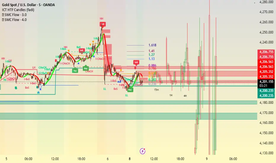
Liquidation Heatmap [Alpha Extract]A sophisticated liquidity zone visualization system that identifies and maps potential liquidation levels based on swing point analysis with volume-weighted intensity measurement and gradient heatmap coloring. Utilizing pivot-based pocket detection and ATR-scaled zone heights, this indicator delivers institutional-grade liquidity mapping with dynamic color intensity reflecting relative liquidity concentration. The system's dual-swing detection architecture combined with configurable weight metrics creates comprehensive liquidation level identification suitable for strategic position planning and market structure analysis.
🔶 Advanced Pivot-Based Pocket Detection
Implements dual swing width analysis to identify potential liquidation zones at pivot highs and lows with configurable lookback periods for comprehensive level coverage. The system detects primary swing points using main pivot width and optional secondary swing detection for increased pocket density, creating layered liquidity maps that capture both major and minor liquidation levels across extended price history.
🔶 Multi-Metric Weight Calculation Engine
Features flexible weight source selection including Volume, Range (high-low spread), and Volume × Range composite metrics for liquidity intensity measurement. The system calculates pocket weights based on market activity at pivot formation, enabling traders to identify which liquidation levels represent higher concentration of potential stops and liquidations with configurable minimum weight thresholds for noise filtering.
🔶 ATR-Based Zone Height Framework
Utilizes Average True Range calculations with percentage-based multipliers to determine pocket vertical dimensions that adapt to market volatility conditions. The system creates ATR-scaled bands above swing highs for short liquidation zones and below swing lows for long liquidation zones, ensuring zone heights remain proportional to current market volatility for accurate level representation.
🔶 Dynamic Gradient Heatmap Visualization
Implements sophisticated color gradient system that maps pocket weights to intensity scales, creating intuitive visual representation of relative liquidity concentration. The system applies power-law transformation with configurable contrast adjustment to enhance differentiation between weak and strong liquidity pockets, using cyan-to-blue gradients for long liquidations and yellow-to-orange for short liquidations.
🔶 Intelligent Pocket State Management
Features advanced pocket tracking system that monitors price interaction with liquidation zones and updates pocket states dynamically. The system detects when price trades through pocket midpoints, marking them as "hit" with optional preservation or removal, and manages pocket extension for untouched levels with configurable forward projection to maintain visibility of approaching liquidity zones.
🔶 Real-Time Liquidity Scale Display
Provides gradient legend showing min-max range of pocket weights with 24-segment color bar for instant liquidity intensity reference. The system positions the scale at chart edge with volume-formatted labels, enabling traders to quickly assess relative strength of visible liquidation pockets without numerical clutter on the main chart area.
🔶 Touched Pocket Border System
Implements visual confirmation of executed liquidations through border highlighting when price trades through pocket zones. The system applies configurable transparency to touched pocket borders with inverted slider logic (lower values fade borders, higher values emphasize them), providing clear historical record of liquidated levels while maintaining focus on active untouched pockets.
🔶 Dual-Swing Density Enhancement
Features optional secondary swing width parameter that creates additional pocket layer with tighter pivot detection for increased liquidation level density. The system runs parallel pivot detection at both primary and secondary swing widths, populating chart with comprehensive liquidity mapping that captures both major swing liquidations and intermediate level clusters.
🔶 Adaptive Pocket Extension Framework
Utilizes intelligent time-based extension that projects untouched pockets forward by configurable bar count, maintaining visibility as price approaches potential liquidation zones. The system freezes touched pocket right edges at hit timestamps while extending active pockets dynamically, creating clear distinction between historical liquidations and forward-projected active levels.
🔶 Weight-Based Label Integration
Provides floating labels on untouched pockets displaying volume-formatted weight values with dynamic positioning that follows pocket extension. The system automatically manages label lifecycle, creating labels for new pockets, updating positions as pockets extend, and removing labels when pockets are touched, ensuring clean chart presentation with relevant liquidity information.
🔶 Performance Optimization Framework
Implements efficient array management with automatic clean-up of old pockets beyond lookback period and optimized box/label deletion to maintain smooth performance. The system includes configurable maximum object counts (500 boxes, 50 labels, 100 lines) with intelligent removal of oldest elements when limits are approached, ensuring consistent operation across extended timeframes.
This indicator delivers sophisticated liquidity zone analysis through pivot-based detection and volume-weighted intensity measurement with intuitive heatmap visualization. Unlike simple support/resistance indicators, the Liquidation Heatmap combines swing point identification with market activity metrics to identify where concentrated liquidations are likely to occur, while the gradient color system instantly communicates relative liquidity strength. The system's dual-swing architecture, configurable weight metrics, ATR-adaptive zone heights, and intelligent state management make it essential for traders seeking strategic position planning around institutional liquidity levels across cryptocurrency, forex, and futures markets. The visual heatmap approach enables instant identification of high-probability reversal zones where cascading liquidations may trigger significant price reactions.

Moving Average ExponentialThe EMA 50 Trend Filter At the heart of the Sniper system lies the 50-period Exponential Moving Average. Unlike simple moving averages, the EMA applies a weighting factor to recent price data, significantly reducing lag. Role in Strategy:
Trend Identification: Serves as the binary divider between Long and Short bias.
Dynamic Structure: Acts as dynamic support in uptrends and resistance in downtrends.
Signal Filtering: The algorithm automatically suppresses any 'Buy' signals below the line and 'Sell' signals above it, ensuring you never trade against the institutional momentum.

Volume Flow Anatomy [Kodexius]Volume Flow Anatomy is a dynamic, multi-dimensional volume map that reconstructs how buy, sell, and “stealth” activity is distributed across price rather than just across time. Instead of relying on a static, session-based volume profile, it uses an exponentially decaying memory of recent bars to build a constantly evolving “anatomy” of the auction, where each price level carries an adaptive history of order flow.
The script separates buy vs. sell pressure, adds a third “Stealth Flow” dimension for low-volume price movement (ease of movement / divergence), and automatically derives POC, Value Area, imbalances, absorption zones, and classic profile shapes (D, P, b, B). This gives the trader a compact but highly information-dense map on the right side of the chart to read control (buyers vs. sellers), structure (balanced vs. trending vs. double distribution), and key reaction levels (support/resistance born from flow, not just wicks).
🔹 Features
🔸 Dynamic Lookback with Decay
- The script computes an effective lookback N from the Decay Factor and caps it with Max Lookback.
- Higher decay keeps more history; lower decay emphasizes the most recent flow.
- The profile continuously adapts as new bars are printed.
🔸 Price-Bucketed Flow Map
Each bucket accumulates:
- Sell Flow (sell pressure)
- Buy Flow (buy pressure)
- Stealth Flow (low-volume price movement)
- Box width at each bucket is proportional to the relative intensity of that component.
🔸 Stealth Flow (Low-Volume Price Movement)
- Measures close to close movement relative to volume, emphasizing price movement that occurs on comparatively low volume.
- Helps reveal hidden participation, inefficient moves, and areas that may be vulnerable to re-tests or reversions.
🔸 POC & 70% Value Area (VA)
- Identifies the Point of Control (price bucket with the highest total volume) over the effective lookback.
- Builds a 70% Value Area by expanding from POC towards the nearest high volume neighbors until 70% of the total volume is included.
- POC is drawn as a line over the analyzed range; VA is displayed as a shaded band in the profile area.
🔸 Market Profile Shape Detection
Splits the profile vertically into three zones (bottom / middle / top) and compares their volume distribution.
Classifies structure as:
- D-Shape (Balanced)
- P-Shape (Short Covering)
- b-Shape (Long Liquidation)
- B-Shape (Double Distribution)
Displays a shape label with color coded bias for quick auction context interpretation.
🔸 Imbalance Zones & Absorption
Imbalance: detects buckets where Buy Flow or Sell Flow exceeds the opposite side by at least Imbalance Ratio.
Absorption: flags zones with high volume but low price “ease”, where price is not moving much despite significant volume.
Extends these levels into horizontal zones, marking potential support/resistance and trap areas.
Bullish Imbalance Zone :
Bearish Imbalance Zone :
Absorption Zone :
🔸 Range Context & On-Chart Legend
Draws a Range Box covering the dynamically determined lookback (N bars), with a label displaying the effective bar count.
A bottom-right legend summarizes:
- Color keys for Buy / Sell / Stealth
- POC / VA status
- Bullish vs. Bearish dominance percentage
- Profile shape classification
- Imbalance and Absorption conventions
🔹 Calculations
1. Dynamic Lookback & Price Buckets
int N = math.min(int(4 / (1 - decayFactor) - 1), maxHistory)
float priceHigh = ta.highest(high, N)
float priceLow = ta.lowest(low, N)
float bucketSize = (priceHigh - priceLow) / bucketCount
The effective lookback N is derived from the Decay Factor, using the approximation 4 / (1 - decay) to capture roughly 99% of the decayed influence, then capped with maxHistory to control performance. Over that adaptive range, the script finds the highest and lowest prices and divides the band into bucketCount equal slices (bucketSize). Each slice is a price bucket that will accumulate volume-flow information.
2. Exponentially Decayed Volume Allocation
addValue(array profile, float weight, float minPrice, float maxPrice) =>
for j = 0 to bucketCount - 1
float bucketMin = priceLow + j * bucketSize
float bucketMax = bucketMin + bucketSize
float overlapMin = math.max(minPrice, bucketMin)
float overlapMax = math.min(maxPrice, bucketMax)
float overlapRange = overlapMax - overlapMin
if overlapRange > 0
profile.set(j, profile.get(j) * decayFactor + weight * overlapRange)
This function is the core engine of the indicator. For a given price span and intensity, it checks every bucket for overlap, distributes the weight proportionally to the overlapping range, and before adding new value, decays the existing bucket content by decayFactor. This results in an exponentially weighted profile: recent activity dominates, while older levels retain a gradually fading footprint.
3. POC and 70% Value Area
array totalProfile = array.new(bucketCount, 0)
for j = 0 to bucketCount - 1
float total = sellProfile.get(j) + buyProfile.get(j)
totalProfile.set(j, total)
if total > eaMax
eaMax := total
int pocIdx = 0
float pocVal = 0.0
for j = 0 to bucketCount - 1
if totalProfile.get(j) > pocVal
pocVal := totalProfile.get(j)
pocIdx := j
float totalSum = totalProfile.sum()
float targetSum = totalSum * 0.70
int vaLow = pocIdx
int vaHigh = pocIdx
float currentSum = pocVal
while currentSum < targetSum and (vaLow > 0 or vaHigh < bucketCount - 1)
float lowVal = vaLow > 0 ? totalProfile.get(vaLow - 1) : 0.0
float highVal = vaHigh < bucketCount - 1 ? totalProfile.get(vaHigh + 1) : 0.0
First, totalProfile is built as the sum of buy and sell flow per bucket, and eaMax (the maximum total) is tracked for later normalization. The POC bucket (pocIdx) is simply the index with the highest totalProfile value.
To compute the 70% Value Area, the algorithm starts at the POC bucket and expands outward, each step adding either the upper or lower neighbor depending on which has more volume. This continues until the cumulative volume reaches 70% of totalSum. The result is a volume-driven VA, not necessarily symmetric around POC, which more accurately represents where the market has truly traded.
4. Market Profile Shape Classification
float volTopThird = 0.0
float volMidThird = 0.0
float volBotThird = 0.0
int thirdIdx = int(bucketCount / 3)
for j = 0 to bucketCount - 1
float val = totalProfile.get(j)
if j < thirdIdx
volBotThird += val
else if j < thirdIdx * 2
volMidThird += val
else
volTopThird += val
float totalVolShape = totalProfile.sum()
string shapeStr = "D-Shape (Balanced)"
if (volTopThird > totalVolShape * 0.20) and (volBotThird > totalVolShape * 0.20) and (volMidThird < totalVolShape * 0.50)
shapeStr := "B-Shape (Double Dist)"
else
if pocIdx > bucketCount * 0.5 and volTopThird > volBotThird * 1.3
shapeStr := "P-Shape (Short Covering)"
else if pocIdx < bucketCount * 0.5 and volBotThird > volTopThird * 1.3
shapeStr := "b-Shape (Long Liquidation)"
else
shapeStr := "D-Shape (Balanced)"
The profile is split into bottom, middle, and top thirds. The script compares how much volume is concentrated in each and combines that with the relative location of POC. If both extremes are heavy and the middle light, it labels a B-Shape (double distribution). If the POC is high and the top dominates the bottom, it’s a P-Shape (short covering). If the POC is low and the bottom dominates, it’s a b-Shape (long liquidation). Otherwise, it defaults to a D-Shape (balanced). This provides a quick, at-a-glance assessment of auction structure.
5. Imbalances, Absorption & Zones
bool isBuyImb = showImb and sVal > 0 and (bVal / sVal >= imbRatio)
bool isSellImb = showImb and bVal > 0 and (sVal / bVal >= imbRatio)
float volRatio = eaMax > 0 ? tVal / eaMax : 0
float stRatio = esmRange > 0 ? (stVal - esmMin) / esmRange : 1.0
bool isAbsorp = showAbsorp and volRatio > 0.6 and stRatio < 0.25
if showImbZone
if isSellImb
zoneBoxes.push(box.new(bar_index - N + 1, bucketHi, bar_index + 1, bucketLo, ...))
if isBuyImb
zoneBoxes.push(box.new(bar_index - N + 1, bucketHi, bar_index + 1, bucketLo, ...))
if isAbsorp
zoneBoxes.push(box.new(bar_index - N + 1, bucketHi, bar_index + 1, bucketLo, ...))
Imbalances are identified where one side’s volume (buy or sell) exceeds the other by at least Imbalance Ratio. These buckets are marked as buy or sell imbalance zones, indicating aggressive participation from one side.
Absorption is detected by combining a high volume ratio (volRatio) with a low normalized stealth ratio (stRatio). High volume with limited price movement suggests that opposing orders are absorbing flow at that level. Both imbalance and absorption buckets are extended into horizontal zones from the start of the lookback to the current bar, visually emphasizing key support/resistance and liquidity areas.
6. Building Buy, Sell & Stealth Profiles
sellProfile := array.new(bucketCount, 0)
buyProfile := array.new(bucketCount, 0)
stealthProfile := array.new(bucketCount, 0)
Three arrays are used to store Sell Flow, Buy Flow, and Stealth Flow. Bars are processed from oldest to newest so that decay is applied in correct chronological order. For each bar, a volume density (volume / range) is calculated and distributed across the candle range. Bull candles feed buyProfile, bear candles feed sellProfile.
Stealth Flow computes the close-to-close move between consecutive bars, scaled by 1 / (1 + volume). Big moves on low volume produce high stealth values, which are then allocated across the move’s price span into stealthProfile. This yields a three-layer profile per price level: directional volume and stealthy price movement.

CRAZY RAY RAY - Dashboard 1-5-15-1D + SMC + Clock + Candles PRO OANDA:XAUUSD This script is essentially your institutional "nuclear power plant" for scalping and swing trading: it combines the 1-5-15-1D dashboard, SMC, PRO candles, money flow times, institutional filters, Bull/Bear 12C, Liquidity HUD, Fibo Move, and Target Trend with SL + 3 TPs into a single indicator. 1. Dashboard 1–5–15–1D (Central HUD)
Calculates across 4 timeframes: 1m, 5m, 15m, and 1D:
Trend with EMAs 15/30/200.
RSI (strength >50 buy, <50 sell).
MACD (crossover in favor or against).
For each timeframe it shows:
TREND → BULLISH / BEARISH / NEUTRAL.
ACTION → BUY / SELL / WAIT.
If all 4 timeframes align:
MODE = BULLISH BUY
MODE = BEARISH SELL
Filters and displays on the HUD if buys or sells are blocked by SMC context (BLOCKED BUY / BLOCKED SELL).
Also draws 2 simple moving averages on the chart:
SMA 20 white (you can use it as a micro-trend).
SMA 200 red (macro trend and institutional reference).
2. Real-Time Clock + Trading Hours
Calculates the real time for:
New York / Miami
London
Tokyo
using current time and real time zone.
Also calculates GMT time to know which session is dominant.
Marks your trading hours:
LONDON 3:00–5:30 (London time) → goodLondon
NY OPEN 8:30–10:00 (NY time) → goodNYOpen
ASIA 20:00–23:00 (Tokyo) → goodAsiaScalp
Displays a message on the HUD:
LONDON 3:00–5:30 (1–2 TRADES)
NY OPEN 8:30–10:00 (1 TRADE)
ASIA 20–23 (SCALP)
NO TRADE ROLL / DEAD / LATE
ONLY A+ SETUPS (when not in strong trading hours).
3. Institutional Power (volume + ATR + session)
Filter that evaluates whether the moment is institutional or retail:
Checks:
If you are in a strong trading session (London / NY). If the volume is above the average × multiplier.
If the ATR is above the average × multiplier.
If it passes the filters → INST ON, otherwise → RETAIL ZONE.
Used internally to block buys/sells and for the HUD.
4. Micro-signal “NO RETRACEMENT” on 1m (BUY SR / SELL SR)
On the 1-minute timeframe, it detects a very aggressive entry:
Clean trend (15/30/200 EMAs aligned).
Price crosses the 200 EMA.
MACD turns in favor.
Marks on the candle:
BUY SR (buys without retracement below the EMA200).
SELL SR (sales without retracement above the EMA200).
This state is also reflected in the HUD as the “SR” row.
5. SMC Block: HH/HL/LH/LL + BMS + ChoCH + Fibo + Zones
This is the SMC brain of the script:
Detects swings with pivots:
Paints HH, HL, LH, LL (if you activate showHHLL).
Marks BOS (break of structure).
Marks BMS and ChoCH (with strong or weak filter using ATR, volume, MACD, gaps).
Draws:
Internal Fibo of the last range (38–50–61).
Fibo entry zone 38–78% as a green discount/premium box.
Institutional mitigation zones (simple OB type green/red boxes).
Current range with dotted yellow lines.
Calculates logic for:
antiStupidBuy: blocks purchases when the context is very bearish (LL–LL–LH, bearish ChoCH, premium, EQH, etc.).
antiStupidSell: symmetrical for sales.
From this comes:
allowBuyInst
allowSellInst
buyBlockerOn / sellBlockerOn
buyTrapDetected (BUY SR signal but context blocks it → BUY TRAP).
All this feeds the HUD and institutional alerts.
6. PRO Candles (candlestick + smart color)
Candlestick pattern system:
Detects:
Hammer, Inverted Hammer. Doji.
Strong bullish/bearish candle.
Bullish/bearish engulfing.
Uses a trend EMA to determine if the pattern is with or against the trend.
Colors the candles according to the pattern (if you enable useColorCandles).
Defines texts:
patternText (pattern name).
biasText (reversal, momentum, indecision).
Updates the HUD with the current pattern (“CANDLE: Engulf Bull”, etc.).
7. Institutional PRO Combo + Reversals
Connects everything:
fullBuySetup:
allowBuyInst TRUE (SMC + Fibo + mitigation OK).
Institutional candles in favor (engulfing, hammer, etc.).
MultiTF aligned (1m, 5m in favor, 15/1D not strongly against).
Strong session (London or NY).
No blockages.
fullSellSetup: the same for sales.
Marks on the chart:
BUY PRO, SELL PRO.
BUY REV LL → reversal from a LL, at Fibo discount, with an institutional candle and above EMA200.
SELL REV HH → reversal from HH, at Fibo premium, with an institutional candle and below EMA200.
And generates alerts for all of this.
8. Dynamic Main HUD
On barstate.islast, updates the HUD:
Changes “BUY / SELL” to:
BUY BLOCK / SELL BLOCK when the context blocks that direction.
Writes:
Current candle pattern.
Time message.
Global status:
BUY TRAP ❌, BUY REV LL ✅, SELL REV HH ✅, BUY PRO ✅, SELL PRO ✅,
BUY BLOCK, SELL BLOCK, BUY/SELL OK.
9. Bull/Bear 12C HUD (Small right HUD)
12-confirmation bull/bear engine:
Calculates:
Sweep, 5th leg, mitigation, HL/LH, strong BOS.
Volume pattern (high-low-high).
ATR rising.
MACD crossover.
Liquidity.
Fear & Greed (SMA50).
Gap/imbalance. Bull/Bear 180 weak.
Count how many are ON:
bullScore /12
bearScore /12
Define a regime:
INSTITUTIONAL → many confirmations + rvol + ATR.
NORMAL
RETAIL
Show on right HUD:
List 1 to 12 with green/red dots BULL / BEAR.
Summary: “Regime: INSTITUTIONAL / NORMAL / RETAIL”.
10. Liquidity HUD XAU SCALP
Calculates RVOL, normalized ATR, spread vs ATR, current range vs average range.
Generates score and classifies:
LOW / MED / HIGH / INS.
Only moves up one level if you are in London/NY session (depending on sessions)

CRR - Smart Money Concept (Pro Expo)Detects Market Structure
Finds pivots using Structure Period.
Marks:
HH (Higher High), LH (Lower High)
HL (Higher Low), LL (Lower Low)
Can draw swing points at highs and lows.
Detects Structure Breaks
When the price breaks the last swing:
BMS (Break of Market Structure) → continuation.
ChoCH (Change of Character) → possible trend reversal.
Differentiates between strong and weak movements using filters.
Confirmation Filters (optional)
If useFilters is enabled, to validate breaks it uses:
ATR → the close must cross the level by at least atrMult * ATR.
Volume → the current volume must be > volMult * average volume.
MACD → in the direction of the break.
Gap → avoids some false breakouts due to gaps.
Internal Fibonacci Retracement of the Last Range
Draws 38.2%, 50%, and 61.8% between the last swing high and swing low.
Serves as internal bounce/discount/premium zones.
Current Range
Draws two dashed yellow lines:
Top: last swing High.
Bottom: last swing Low.
Shows you the range where the price is currently trading.
🧩 In short:
This script draws complete SMC structure (HH/HL/LL/LH + BMS + ChoCH), validates breakouts with ATR, volume, MACD, and gaps, and also displays internal Fibonacci retracement + current range, all automatically and cleanly.

Stop Hunt / Liquidity Sweep Detector with Momentum Ratingdetects liquidity sweeps as they happen then gives you a rating on how much momentum the reversal has.

T-DOW-FLOW: Final Edition
T-DOW-FLOW: Market Structure & Smart Pivot Zones
This indicator is a comprehensive technical analysis tool designed to visualize "Market Structure" based on Dow Theory and precise Supply/Demand Zones. It helps traders identify the true market trend and high-probability reaction levels by analyzing raw price action (ZigZag Pivots) rather than lagging indicators.
The script integrates three core systems:
ZigZag Trend Cloud: Visualizes the market bias (Uptrend/Downtrend).
Smart Pivot Zones (Type 1): Highlights the specific "Wick-to-Body" area of recent pivots.
Auto Density Channels (Type 2): Detects historical support/resistance clusters.
1. ZigZag Trend Identification
Logic: The script utilizes ta.highestbars and ta.lowestbars to detect Swing Highs and Swing Lows.
Trend Cloud:
If the structure creates a Higher High, the background cloud turns Green (Uptrend).
If the structure creates a Lower Low, the background cloud turns Red (Downtrend).
This provides an instant visual filter for "Trend Flow," encouraging traders to trade only in the direction of the dominant market structure.
2. SR Type 1: Smart Pivot Zones (Wick-to-Body)
Unlike standard indicators that draw thin lines at the absolute High/Low, this script focuses on the "Imbalance Zone".
It calculates the price range between the Pivot's Wick and the Pivot's Body (Open/Close) and fills this area with a colored zone.
Why? The area between the wick and body often represents the precise zone where institutional orders were filled, acting as a more reliable support/resistance level than a single price point.
3. SR Type 2: Auto Density Channels
This module scans a significant amount of historical data (default: 300 bars) to find clusters of pivot points.
Areas where multiple pivots align within a specific width are drawn as Channels. These represent strong, long-term psychological levels.
Trend Filter: Check the Trend Cloud color.
Green: Look for Long opportunities.
Red: Look for Short opportunities.
Entry Trigger: Wait for the price to retrace into a Smart Pivot Zone (Type 1) or an Auto Channel (Type 2).
Look for price rejection (wicks) at these zones in the direction of the Trend Cloud.
Structure Confirmation: Use the ZigZag lines and labels (HH, HL, etc.) to confirm that the market structure is still intact before entering.
ZigZag Settings: Adjust the sensitivity of the trend detection.
SR Type 1: Toggle the "Wick-to-Body" fill and choose between Wicks or Bodies as the primary source.
SR Type 2: Adjust the historical loopback period and channel width sensitivity.
This script is for educational and technical analysis purposes only. Past performance does not guarantee future results.
(以下、日本語説明 / Japanese Description)
このインジケーターは、「ダウ理論」に基づくトレンド判定と、精密な「需給ゾーン(Supply/Demand)」を可視化するための市場構造分析ツールです。 遅行指標を使わず、純粋なプライスアクション(ZigZagピボット)に基づいて、機関投資家の意識する価格帯を特定します。
1. ZigZagトレンドクラウド
ロジック: 一定期間の高値・安値を検出し、ダウ理論に基づいてトレンドを判定します。
視覚化: 高値切り上げ(上昇トレンド)なら「緑」、安値切り下げ(下落トレンド)なら「赤」の背景色を表示します。これにより、トレードすべき方向(順張り)を一目で判断できます。
2. SR Type 1: スマートピボットゾーン (Wick-to-Body)
単なる水平線ではなく、ローソク足の**「ヒゲ先」から「実体」までの価格差**をゾーンとして塗りつぶして表示します。
理由: ヒゲと実体の間の領域は、大口の注文が執行された(需給の不均衡が発生した)重要なエリアであることが多く、ピンポイントのラインよりも信頼性の高い反発ゾーンとして機能します。
3. SR Type 2: オート・デンシティ・チャネル
過去の長期間(デフォルト300本)のデータをスキャンし、ピボットが密集している価格帯を自動で「チャネル」として描画します。長期的に意識される強力なレジサポ帯です。
環境認識: 背景のトレンドクラウドの色に従い、目線を固定します。
エントリー: 価格がSRゾーン(Type 1)やチャネル(Type 2)に引きつけて、反発する動きを確認してエントリーします。
構造確認: ZigZagラインとラベル(HH/HLなど)を見て、トレンドが崩れていないことを確認します。

Volatility Risk PremiumTHE INSURANCE PREMIUM OF THE STOCK MARKET
Every day, millions of investors face a fundamental question that has puzzled economists for decades: how much should protection against market crashes cost? The answer lies in a phenomenon called the Volatility Risk Premium, and understanding it may fundamentally change how you interpret market conditions.
Think of the stock market like a neighborhood where homeowners buy insurance against fire. The insurance company charges premiums based on their estimates of fire risk. But here is the interesting part: insurance companies systematically charge more than the actual expected losses. This difference between what people pay and what actually happens is the insurance premium. The same principle operates in financial markets, but instead of fire insurance, investors buy protection against market volatility through options contracts.
The Volatility Risk Premium, or VRP, measures exactly this difference. It represents the gap between what the market expects volatility to be (implied volatility, as reflected in options prices) and what volatility actually turns out to be (realized volatility, calculated from actual price movements). This indicator quantifies that gap and transforms it into actionable intelligence.
THE FOUNDATION
The academic study of volatility risk premiums began gaining serious traction in the early 2000s, though the phenomenon itself had been observed by practitioners for much longer. Three research papers form the backbone of this indicator's methodology.
Peter Carr and Liuren Wu published their seminal work "Variance Risk Premiums" in the Review of Financial Studies in 2009. Their research established that variance risk premiums exist across virtually all asset classes and persist over time. They documented that on average, implied volatility exceeds realized volatility by approximately three to four percentage points annualized. This is not a small number. It means that sellers of volatility insurance have historically collected a substantial premium for bearing this risk.
Tim Bollerslev, George Tauchen, and Hao Zhou extended this research in their 2009 paper "Expected Stock Returns and Variance Risk Premia," also published in the Review of Financial Studies. Their critical contribution was demonstrating that the VRP is a statistically significant predictor of future equity returns. When the VRP is high, meaning investors are paying substantial premiums for protection, future stock returns tend to be positive. When the VRP collapses or turns negative, it often signals that realized volatility has spiked above expectations, typically during market stress periods.
Gurdip Bakshi and Nikunj Kapadia provided additional theoretical grounding in their 2003 paper "Delta-Hedged Gains and the Negative Market Volatility Risk Premium." They demonstrated through careful empirical analysis why volatility sellers are compensated: the risk is not diversifiable and tends to materialize precisely when investors can least afford losses.
HOW THE INDICATOR CALCULATES VOLATILITY
The calculation begins with two separate measurements that must be compared: implied volatility and realized volatility.
For implied volatility, the indicator uses the CBOE Volatility Index, commonly known as the VIX. The VIX represents the market's expectation of 30-day forward volatility on the S&P 500, calculated from a weighted average of out-of-the-money put and call options. It is often called the "fear gauge" because it rises when investors rush to buy protective options.
Realized volatility requires more careful consideration. The indicator offers three distinct calculation methods, each with specific advantages rooted in academic literature.
The Close-to-Close method is the most straightforward approach. It calculates the standard deviation of logarithmic daily returns over a specified lookback period, then annualizes this figure by multiplying by the square root of 252, the approximate number of trading days in a year. This method is intuitive and widely used, but it only captures information from closing prices and ignores intraday price movements.
The Parkinson estimator, developed by Michael Parkinson in 1980, improves efficiency by incorporating high and low prices. The mathematical formula calculates variance as the sum of squared log ratios of daily highs to lows, divided by four times the natural logarithm of two, times the number of observations. This estimator is theoretically about five times more efficient than the close-to-close method because high and low prices contain additional information about the volatility process.
The Garman-Klass estimator, published by Mark Garman and Michael Klass in 1980, goes further by incorporating opening, high, low, and closing prices. The formula combines half the squared log ratio of high to low prices minus a factor involving the log ratio of close to open. This method achieves the minimum variance among estimators using only these four price points, making it particularly valuable for markets where intraday information is meaningful.
THE CORE VRP CALCULATION
Once both volatility measures are obtained, the VRP calculation is straightforward: subtract realized volatility from implied volatility. A positive result means the market is paying a premium for volatility insurance. A negative result means realized volatility has exceeded expectations, typically indicating market stress.
The raw VRP signal receives slight smoothing through an exponential moving average to reduce noise while preserving responsiveness. The default smoothing period of five days balances signal clarity against lag.
INTERPRETING THE REGIMES
The indicator classifies market conditions into five distinct regimes based on VRP levels.
The EXTREME regime occurs when VRP exceeds ten percentage points. This represents an unusual situation where the gap between implied and realized volatility is historically wide. Markets are pricing in significantly more fear than is materializing. Research suggests this often precedes positive equity returns as the premium normalizes.
The HIGH regime, between five and ten percentage points, indicates elevated risk aversion. Investors are paying above-average premiums for protection. This often occurs after market corrections when fear remains elevated but realized volatility has begun subsiding.
The NORMAL regime covers VRP between zero and five percentage points. This represents the long-term average state of markets where implied volatility modestly exceeds realized volatility. The insurance premium is being collected at typical rates.
The LOW regime, between negative two and zero percentage points, suggests either unusual complacency or that realized volatility is catching up to implied volatility. The premium is shrinking, which can precede either calm continuation or increased stress.
The NEGATIVE regime occurs when realized volatility exceeds implied volatility. This is relatively rare and typically indicates active market stress. Options were priced for less volatility than actually occurred, meaning volatility sellers are experiencing losses. Historically, deeply negative VRP readings have often coincided with market bottoms, though timing the reversal remains challenging.
TERM STRUCTURE ANALYSIS
Beyond the basic VRP calculation, sophisticated market participants analyze how volatility behaves across different time horizons. The indicator calculates VRP using both short-term (default ten days) and long-term (default sixty days) realized volatility windows.
Under normal market conditions, short-term realized volatility tends to be lower than long-term realized volatility. This produces what traders call contango in the term structure, analogous to futures markets where later delivery dates trade at premiums. The RV Slope metric quantifies this relationship.
When markets enter stress periods, the term structure often inverts. Short-term realized volatility spikes above long-term realized volatility as markets experience immediate turmoil. This backwardation condition serves as an early warning signal that current volatility is elevated relative to historical norms.
The academic foundation for term structure analysis comes from Scott Mixon's 2007 paper "The Implied Volatility Term Structure" in the Journal of Derivatives, which documented the predictive power of term structure dynamics.
MEAN REVERSION CHARACTERISTICS
One of the most practically useful properties of the VRP is its tendency to mean-revert. Extreme readings, whether high or low, tend to normalize over time. This creates opportunities for systematic trading strategies.
The indicator tracks VRP in statistical terms by calculating its Z-score relative to the trailing one-year distribution. A Z-score above two indicates that current VRP is more than two standard deviations above its mean, a statistically unusual condition. Similarly, a Z-score below negative two indicates VRP is unusually low.
Mean reversion signals trigger when VRP reaches extreme Z-score levels and then shows initial signs of reversal. A buy signal occurs when VRP recovers from oversold conditions (Z-score below negative two and rising), suggesting that the period of elevated realized volatility may be ending. A sell signal occurs when VRP contracts from overbought conditions (Z-score above two and falling), suggesting the fear premium may be excessive and due for normalization.
These signals should not be interpreted as standalone trading recommendations. They indicate probabilistic conditions based on historical patterns. Market context and other factors always matter.
MOMENTUM ANALYSIS
The rate of change in VRP carries its own information content. Rapidly rising VRP suggests fear is building faster than volatility is materializing, often seen in the early stages of corrections before realized volatility catches up. Rapidly falling VRP indicates either calming conditions or rising realized volatility eating into the premium.
The indicator tracks VRP momentum as the difference between current VRP and VRP from a specified number of bars ago. Positive momentum with positive acceleration suggests strengthening risk aversion. Negative momentum with negative acceleration suggests intensifying stress or rapid normalization from elevated levels.
PRACTICAL APPLICATION
For equity investors, the VRP provides context for risk management decisions. High VRP environments historically favor equity exposure because the market is pricing in more pessimism than typically materializes. Low or negative VRP environments suggest either reducing exposure or hedging, as markets may be underpricing risk.
For options traders, understanding VRP is fundamental to strategy selection. Strategies that sell volatility, such as covered calls, cash-secured puts, or iron condors, tend to profit when VRP is elevated and compress toward its mean. Strategies that buy volatility tend to profit when VRP is low and risk materializes.
For systematic traders, VRP provides a regime filter for other strategies. Momentum strategies may benefit from different parameters in high versus low VRP environments. Mean reversion strategies in VRP itself can form the basis of a complete trading system.
LIMITATIONS AND CONSIDERATIONS
No indicator provides perfect foresight, and the VRP is no exception. Several limitations deserve attention.
The VRP measures a relationship between two estimates, each subject to measurement error. The VIX represents expectations that may prove incorrect. Realized volatility calculations depend on the chosen method and lookback period.
Mean reversion tendencies hold over longer time horizons but provide limited guidance for short-term timing. VRP can remain extreme for extended periods, and mean reversion signals can generate losses if the extremity persists or intensifies.
The indicator is calibrated for equity markets, specifically the S&P 500. Application to other asset classes requires recalibration of thresholds and potentially different data sources.
Historical relationships between VRP and subsequent returns, while statistically robust, do not guarantee future performance. Structural changes in markets, options pricing, or investor behavior could alter these dynamics.
STATISTICAL OUTPUTS
The indicator presents comprehensive statistics including current VRP level, implied volatility from VIX, realized volatility from the selected method, current regime classification, number of bars in the current regime, percentile ranking over the lookback period, Z-score relative to recent history, mean VRP over the lookback period, realized volatility term structure slope, VRP momentum, mean reversion signal status, and overall market bias interpretation.
Color coding throughout the indicator provides immediate visual interpretation. Green tones indicate elevated VRP associated with fear and potential opportunity. Red tones indicate compressed or negative VRP associated with complacency or active stress. Neutral tones indicate normal market conditions.
ALERT CONDITIONS
The indicator provides alerts for regime transitions, extreme statistical readings, term structure inversions, mean reversion signals, and momentum shifts. These can be configured through the TradingView alert system for real-time monitoring across multiple timeframes.
REFERENCES
Bakshi, G., and Kapadia, N. (2003). Delta-Hedged Gains and the Negative Market Volatility Risk Premium. Review of Financial Studies, 16(2), 527-566.
Bollerslev, T., Tauchen, G., and Zhou, H. (2009). Expected Stock Returns and Variance Risk Premia. Review of Financial Studies, 22(11), 4463-4492.
Carr, P., and Wu, L. (2009). Variance Risk Premiums. Review of Financial Studies, 22(3), 1311-1341.
Garman, M. B., and Klass, M. J. (1980). On the Estimation of Security Price Volatilities from Historical Data. Journal of Business, 53(1), 67-78.
Mixon, S. (2007). The Implied Volatility Term Structure of Stock Index Options. Journal of Empirical Finance, 14(3), 333-354.
Parkinson, M. (1980). The Extreme Value Method for Estimating the Variance of the Rate of Return. Journal of Business, 53(1), 61-65.

RVOL + Volume Z-Score (Textbook)This indicator is a relative-volume and “volume anomaly” dashboard designed to help you quickly spot when a ticker is actually in-play versus simply drifting on normal activity. It plots standard volume bars (colored by up/down candles) and overlays multiple optional smoothers of volume (SMA, LSMA/linear-regression MA, HMA, ALMA) so you can see whether participation is expanding or fading across different smoothing styles. It also calculates RVOL (current bar volume divided by the average volume over a user-defined lookback) and displays RVOL (and Z) in a small table for quick reference.
The core feature is a textbook volume z-score: Z=(V−SMA(V,N))/StDev(V,N)
This measures how far the current bar’s volume is from its recent average in standard-deviation units, making it easy to filter for genuinely unusual volume. The script plots mean + 1σ and mean + 2σ threshold bands and can highlight “anomaly” volume bars when Z exceeds your chosen σ thresholds (default 1σ for broader detection, with alerts available for 1σ/2σ). Use it as a participation filter: combine high RVOL / high Z with your price structure (key levels, VWAP, trend) to validate breakouts or identify high-conviction reversal/flush events.
Trend Tracer [AlgoAlpha]🟠 OVERVIEW
This tool builds a two-stage trend model that reacts to structure shifts while also showing how strong or weak the move is. It uses a mid-price band (from the highest high and lowest low over a lookback) and applies two Supertrend passes on top of it. The first pass smoothens the basis. The second pass refines that direction and produces the final trail used for signals. A gradient fill between the two trails uses RSI of price-to-trail distance to show when price is stretched or cooling off. The aim is to give traders a simple way to read trend alignment, pressure, and early turns without guessing.
🟠 CONCEPTS
The script starts with a mid-range basis. This is the average of the rolling highest high and lowest low. It acts as a stable structure reference instead of raw close or typical price. From there, two Supertrend layers are applied:
• The first Supertrend uses a shorter ATR period and lower factor. It reacts faster and sets the main regime.
• The second Supertrend uses a slightly longer ATR and higher factor. It filters noise, waits for confirmed continuation, and generates the signal line.
The interaction between these trails matters. The outer Supertrend provides context by defining the broader regime. The inner Supertrend provides timing by flipping earlier and marking possible shifts. The gradient fill uses RSI of (close − supertrend value) to display when price stretches away from the trail. This shows strength, exhaustion, or compression within the trend.
🟠 FEATURES
Bullish and bearish flip markers placed at recent highs/lows
Rejection signals off the trend tracer line
Alerts for bullish and bearish trend changes
🟠 USAGE
Setup : Add the script to your chart. Timeframe is flexible; lower timeframes show more flips while higher ones give cleaner swings. Adjust Length to change how wide the basis range is. Use the two ATR settings and factors to match the volatility of the market you trade.
Read the chart : When the refined trail (stv_) sits above price the regime is bearish; when below, it is bullish. The wide trail (stv) confirms the larger move. Watch the gradient fill: darker colors appear when price is stretched from the trail and lighter colors appear when the move is weakening. Flip markers ▲ or ▼ highlight the first clean shift of the refined trail.
Settings that matter : Increasing the Main Factor slows main-trend flips and filters chop. Increasing the Signal Factor delays the timing trail but reduces noise. Shortening Length makes the basis more reactive. ATR periods change how sensitive each Supertrend pass is to volatility.