TASC 2025.07 Laguerre Filters█ OVERVIEW
This script implements the Laguerre filter and oscillator described by John F. Ehlers in the article "A Tool For Trend Trading, Laguerre Filters" from the July 2025 edition of TASC's Traders' Tips . The new Laguerre filter utilizes the UltimateSmoother filter in place of an exponential moving average (EMA) in its calculation, offering improved responsiveness and reduced lag.
█ CONCEPTS
As Ehlers explains in his article, the Laguerre filter is a form of transversal filter . A transversal filter calculates an output signal using a tapped delay line . It creates multiple delayed versions of an input signal, applies weight to each delay, and then calculates their sum to generate the filtered result.
The Laguerre filter's structure relies on Laguerre polynomials — solutions to a differential equation solved by Edmond Laguerre in the 1800s. When Ehlers analyzed the formula for these polynomials on discrete systems (e.g., financial time series), he found that the first term's expression corresponds to an EMA response, and all subsequent terms correspond to an all-pass response. In contrast to other filter types, an all-pass filter produces phase shift (i.e., delay) in an input signal's components without affecting its amplitude.
Ehlers observed that these characteristics of Laguerre polynomials make them suitable for use in a transversal filter structure, and thus the Laguerre filter was born. However, he notes that EMAs are not great filters in general. As such, to improve on the Laguerre filter's design, Ehlers modified it by replacing the EMA term with his UltimateSmoother filter. The resulting Laguerre filter has significantly reduced lag, achieving a tighter response to market fluctuations while maintaining smoothness. Ehlers suggests that traders can analyze crossings between the UltimateSmoother and this Laguerre filter, or those between two Laguerre filters of different order, for helpful buy and sell signals.
In addition to the Laguerre filter, Ehlers derived a smooth, low-lag oscillator based on the difference between the first and second terms in the modified filter structure, scaled by the root mean square (RMS). The resulting oscillator provides an alternative filtered representation of market data, which can help traders identify swing and mean-reversion signals.
█ USAGE
This indicator calculates both the Laguerre filter and the Laguerre oscillator described in Ehlers' article. It displays the Laguerre filter on the main chart pane and the oscillator in a separate pane.
Users can control the behavior of the filter and oscillator with the inputs in the "Settings/Inputs" tab:
The "Period" input defines the critical period of the UltimateSmoother used in the Laguerre filter and oscillator calculations. Its default value is 30.
The "Gamma" input determines the weighting behavior of the Laguerre filter and oscillator. It accepts a positive value between 0 and 1. Use a lower value for quicker responsiveness to market changes, and a higher value for trends. The default value is 0.5.
The "RMS length" input determines the length of the RMS calculation for oscillator normalization. The default value is 100 bars.
Cari skrip untuk "上证指数+2025年4月8日+收盘价"

BackToBasic XEMAบทความอธิบายสคริปต์ “BackToBasic XEMA”
ภาษาไทย
แนวคิดโดยย่อ
BackToBasic XEMA เกิดจากแนวคิด “กลับสู่พื้นฐานแต่เพิ่มประโยชน์” โดยใช้สัญญาณ EMA Crossover เป็นแกนหลัก แล้วต่อยอดด้วยการแสดงกำไร/ขาดทุนจริง (PnL) และเส้น Trailing Stop แนวนอน เพื่อช่วยวัดประสิทธิภาพและป้องกันการคืนกำไร
กลไกการทำงาน
Dual EMA – คำนวณ EMA สองเส้น (Fast และ Slow)
Crossover Signal – ออกสัญญาณ Buy เมื่อ Fast ตัดขึ้น Slow และ Sell เมื่อ Fast ตัดลง Slow
PnL Lines & Labels – เมื่อทิศทางกลับตัว ระบบจะคำนวณส่วนต่างราคา × จำนวน Contracts แล้ววาดเส้นเชื่อมจุดเข้า–ออก พร้อมป้ายกำไร/ขาดทุนสีเขียว / แดง
Horizontal Trailing Stop – เมื่อราคาวิ่งไปทางกำไรเกิน trailStartPips ระบบจะสร้างเส้น Trail ห่างจาก EMA อ้างอิงด้วย trailBufferPips และเลื่อนเฉพาะในทางที่ล็อกกำไร
การตั้งค่าใช้งาน (สรุปเป็นคำอธิบาย)
ปรับค่า Fast/Slow EMA ให้สัมพันธ์กับกรอบเวลาและความผันผวนของสินทรัพย์
กรอกจำนวน Contracts ตามขนาดโพซิชันจริงเพื่อให้ค่า PnL สมจริง
ค่า Trail เริ่มต้นเหมาะกับกราฟ 1 ชั่วโมงขึ้นไป หากเทรดสั้นอาจลด trailStartPips และ trailBufferPips
แนะนำใช้กับสินทรัพย์สภาพคล่องสูง (คู่เงินหลัก, XAUUSD, ดัชนี) และทดสอบบนบัญชีเดโมก่อนเสมอ
จุดเด่นเมื่อเทียบกับ EMA Crossover พื้นฐาน
เห็นผลกำไร/ขาดทุนของแต่ละการเทรดทันที ไม่ต้องคำนวณย้อนหลัง
มีเส้น Trailing Stop แนวนอนช่วยล็อกกำไรและจำกัดขาดทุน
เปิด–ปิดฟังก์ชัน PnL และ Trailing ได้จากหน้าตั้งค่า ไม่ยุ่งยาก
ข้อจำกัดและคำเตือน
ไม่เหมาะกับกราฟแบบ Heikin Ashi หรือ Renko เพราะอาจเกิด repaint
PnL คำนวณจากส่วนต่างราคาเท่านั้น ไม่รวมค่าคอมมิชชันหรือสลิปเพจ
ผลลัพธ์ในอดีตไม่รับประกันอนาคต ควรจัดการความเสี่ยงและทดลองก่อนใช้งานจริง
ลิขสิทธิ์
สคริปต์นี้พัฒนาใหม่ทั้งหมดโดย , © 2025
English
Concept
BackToBasic XEMA extends a classic EMA-crossover setup with real-time profit-and-loss tracking and a horizontal trailing-stop line, giving traders both clear entry/exit signals and built-in risk management.
How It Works
Dual EMAs – Calculates Fast and Slow EMAs.
Crossover Signals – Generates a Buy when the Fast EMA crosses above the Slow EMA, and a Sell when it crosses below.
PnL Lines & Labels – On every direction flip the script computes price difference × contracts, draws a line from entry to exit, and labels the result in green (profit) or red (loss).
Horizontal Trailing Stop – After price moves in profit by at least trailStartPips, a trail line is placed trailBufferPips away from the chosen EMA and moves only in the trade’s favour.
Practical Settings (plain-language guide)
Adjust Fast/Slow EMA lengths to suit your timeframe and the instrument’s volatility.
Enter your position size in Contracts so PnL lines reflect real cash values.
For shorter timeframes, lower trailStartPips and trailBufferPips; for swing trading, larger values work better.
Best used on 1-hour-and-above charts of liquid symbols (major FX pairs, gold, indices). Forward-test on demo first.
Advantages over a Basic EMA Cross
Instant visual feedback on each trade’s profit or loss.
Built-in horizontal trailing stop to lock in gains and limit downside.
Modular design – PnL and trailing features can be toggled on or off in the input panel.
Limitations & Disclaimer
Not repaint-safe on non-standard chart types such as Heikin Ashi or Renko.
PnL lines show raw price change only; commissions and slippage are not included.
Past performance does not guarantee future results – trade responsibly and test thoroughly.
License
Original Pine Script by , © 2025

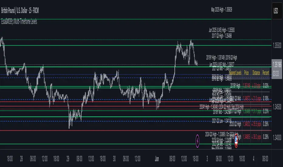
Essa - Multi-Timeframe LevelsEnhanced Multi‐Timeframe Levels
This indicator plots yearly, quarterly and monthly highs, lows and midpoints on your chart. Each level is drawn as a horizontal line with an optional label showing “ – ” (for example “Apr 2025 High – 1.2345”). If two or more timeframes share the same price (within two ticks), they are merged into a single line and the label lists each timeframe.
A distance table can be shown in any corner of the chart. It lists up to five active levels closest to the current closing price and shows for each level:
level name (e.g. “May 2025 Low”)
exact price
distance in pips or points (calculated according to the instrument’s tick size)
percentage difference relative to the close
Alerts can be enabled so that whenever price comes within a user-specified percentage of any level (for example 0.1 %), an alert fires. Once price decisively crosses a level, that level is marked as “broken” so it does not trigger again. Built-in alertcondition hooks are also provided for definite breaks of the current monthly, quarterly and yearly highs and lows.
Monthly lookback is configurable (default 6 months), and once the number of levels exceeds a cap (calculated as 20 + monthlyLookback × 3), the oldest levels are automatically removed to avoid clutter. Line widths and colours (with adjustable opacity for quarterly and monthly) can be set separately for each timeframe. Touches of each level are counted internally to allow future extension (for example visually emphasising levels with multiple touches).
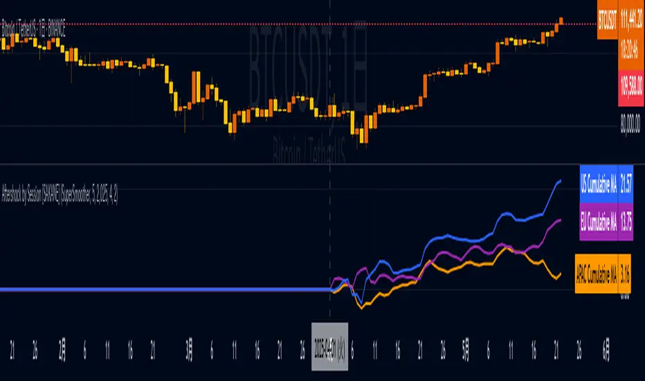
Aftershock by Session [SAKANE]■ Background & Motivation
In 24/7 markets like crypto, not all participants react simultaneously to major events.
Instead, reactions unfold across different regional trading sessions — Asia (APAC), Europe (EU), and the United States (US) — each with its own tempo and sentiment.
This indicator is designed to visualize which session drives the market after a key event — capturing the "aftershock" effect that ripples through time zones.
■ Key Features
Tracks price return (open → close) for each session: APAC / EU / US
Cumulative session returns are calculated and visualized
Smoothing options: SMA, EMA, or Ehlers SuperSmoother
Optimized for daily charts to highlight structural momentum shifts
Toggle visibility of each session independently
■ Why “Aftershock”?
Take April 2, 2025 — the day of the “Trump Tariff Opening.”
That policy announcement triggered a market-wide response. But:
Which session reacted first?
Which session truly moved the market?
This indicator is named “Aftershock” because it helps you see the ripple effect of such events — when and where momentum followed.
■ How to Use
Search for “Aftershock by Session ” on TradingView
Add it to your chart (use Daily timeframe)
Customize sessions and smoothing options via settings
You can also bookmark it for quick access.
■ Insights & Use Cases
Detect which session initiated or led market moves after news events
Understand geo-temporal dynamics — did the move start in Asia, Europe, or the US?
For example, on April 2, 2025, the day Trump’s tariff pivot was announced:
You can instantly see which session took the lead —
the APAC session hesitated, while the US session drove the trend.
This insight becomes visually obvious with the cumulative lines.
■ Unique Value
Unlike typical indicators based on raw price action,
Aftershock analyzes market movement through a session-based structural lens.
It captures where capital actually moved — and when.
A tool not just for technical analysis, but for event-driven, macro-aware market reading.
■ Final Thoughts
To truly understand market mechanics, we must look beyond candles and trends.
Aftershock by Session breaks down the 24-hour cycle into meaningful regional flows,
allowing you to track the true drivers behind price momentum.
Whether you're trading, researching, or tracking macro catalysts,
this tool helps answer the key question:
“Who moved the market — and when?”
TASC 2025.06 Cybernetic Oscillator█ OVERVIEW
This script implements the Cybernetic Oscillator introduced by John F. Ehlers in his article "The Cybernetic Oscillator For More Flexibility, Making A Better Oscillator" from the June 2025 edition of the TASC Traders' Tips . It cascades two-pole highpass and lowpass filters, then scales the result by its root mean square (RMS) to create a flexible normalized oscillator that responds to a customizable frequency range for different trading styles.
█ CONCEPTS
Oscillators are indicators widely used by technical traders. These indicators swing above and below a center value, emphasizing cyclic movements within a frequency range. In his article, Ehlers explains that all oscillators share a common characteristic: their calculations involve computing differences . The reliance on differences is what causes these indicators to oscillate about a central point.
The difference between two data points in a series acts as a highpass filter — it allows high frequencies (short wavelengths) to pass through while significantly attenuating low frequencies (long wavelengths). Ehlers demonstrates that a simple difference calculation attenuates lower-frequency cycles at a rate of 6 dB per octave. However, the difference also significantly amplifies cycles near the shortest observable wavelength, making the result appear noisier than the original series. To mitigate the effects of noise in a differenced series, oscillators typically smooth the series with a lowpass filter, such as a moving average.
Ehlers highlights an underlying issue with smoothing differenced data to create oscillators. He postulates that market data statistically follows a pink spectrum , where the amplitudes of cyclic components in the data are approximately directly proportional to the underlying periods. Specifically, he suggests that cyclic amplitude increases by 6 dB per octave of wavelength.
Because some conventional oscillators, such as RSI, use differencing calculations that attenuate cycles by only 6 dB per octave, and market cycles increase in amplitude by 6 dB per octave, such calculations do not have a tangible net effect on larger wavelengths in the analyzed data. The influence of larger wavelengths can be especially problematic when using these oscillators for mean reversion or swing signals. For instance, an expected reversion to the mean might be erroneous because oscillator's mean might significantly deviate from its center over time.
To address the issues with conventional oscillator responses, Ehlers created a new indicator dubbed the Cybernetic Oscillator. It uses a simple combination of highpass and lowpass filters to emphasize a specific range of frequencies in the market data, then normalizes the result based on RMS. The process is as follows:
Apply a two-pole highpass filter to the data. This filter's critical period defines the longest wavelength in the oscillator's passband.
Apply a two-pole SuperSmoother (lowpass filter) to the highpass-filtered data. This filter's critical period defines the shortest wavelength in the passband.
Scale the resulting waveform by its RMS. If the filtered waveform follows a normal distribution, the scaled result represents amplitude in standard deviations.
The oscillator's two-pole filters attenuate cycles outside the desired frequency range by 12 dB per octave. This rate outweighs the apparent rate of amplitude increase for successively longer market cycles (6 dB per octave). Therefore, the Cybernetic Oscillator provides a more robust isolation of cyclic content than conventional oscillators. Best of all, traders can set the periods of the highpass and lowpass filters separately, enabling fine-tuning of the frequency range for different trading styles.
█ USAGE
The "Highpass period" input in the "Settings/Inputs" tab specifies the longest wavelength in the oscillator's passband, and the "Lowpass period" input defines the shortest wavelength. The oscillator becomes more responsive to rapid movements with a smaller lowpass period. Conversely, it becomes more sensitive to trends with a larger highpass period. Ehlers recommends setting the smallest period to a value above 8 to avoid aliasing. The highpass period must not be smaller than the lowpass period. Otherwise, it causes a runtime error.
The "RMS length" input determines the number of bars in the RMS calculation that the indicator uses to normalize the filtered result.
This indicator also features two distinct display styles, which users can toggle with the "Display style" input. With the "Trend" style enabled, the indicator plots the oscillator with one of two colors based on whether its value is above or below zero. With the "Threshold" style enabled, it plots the oscillator as a gray line and highlights overbought and oversold areas based on the user-specified threshold.
Below, we show two instances of the script with different settings on an equities chart. The first uses the "Threshold" style with default settings to pass cycles between 20 and 30 bars for mean reversion signals. The second uses a larger highpass period of 250 bars and the "Trend" style to visualize trends based on cycles spanning less than one year:

EXODUS EXODUS by (DAFE) Trading Systems
EXODUS is a sophisticated trading algorithm built by Dskyz (DAFE) Trading Systems for competitive and competition purposes, designed to identify high-probability trades with robust risk management. this strategy leverages a multi-signal voting system, combining three core components—SPR, VWMO, and VEI—alongside ADX, choppiness filters, and ATR-based volatility gates to ensure trades are taken only in favorable market conditions. the algo uses a take-profit to stop-loss ratio, dynamic position sizing, and a strict voting mechanism requiring all signals to align before entering a trade.
EXODUS was not overfitted for any specific symbol. instead, it uses a generic tuned setting, making it versatile across various markets. while it can trade futures, it’s not currently set up for it but has the potential to do more with further development. visuals are intentionally minimal due to its competition focus, prioritizing performance over aesthetics. a more visually stunning version may be released in the future with enhanced graphics.
The Unique Core Components Developed for EXODUS
SPR (Session Price Recalibration)
SPR measures momentum during regular trading hours (RTH, 0930-1600, America/New_York) to catch session-specific trends.
spr_lookback = input.int(15, "SPR Lookback") this sets how many bars back SPR looks to calculate momentum (default 15 bars). it compares the current session’s price-volume score to the score 15 bars ago to gauge momentum strength.
how it works: a longer lookback smooths out the signal, focusing on bigger trends. a shorter one makes SPR more sensitive to recent moves.
how to adjust: on a 1-hour chart, 15 bars is 15 hours (about 2 trading days). if you’re on a shorter timeframe like 5 minutes, 15 bars is just 75 minutes, so you might want to increase it to 50 or 100 to capture more meaningful trends. if you’re trading a choppy stock, a shorter lookback (like 5) can help catch quick moves, but it might give more false signals.
spr_threshold = input.float (0.7, "SPR Threshold")
this is the cutoff for SPR to vote for a trade (default 0.7). if SPR’s normalized value is above 0.7, it votes for a long; below -0.7, it votes for a short.
how it works: SPR normalizes its momentum score by ATR, so this threshold ensures only strong moves count. a higher threshold means fewer trades but higher conviction.
how to adjust: if you’re getting too few trades, lower it to 0.5 to let more signals through. if you’re seeing too many false entries, raise it to 1.0 for stricter filtering. test on your chart to find a balance.
spr_atr_length = input.int(21, "SPR ATR Length") this sets the ATR period (default 21 bars) used to normalize SPR’s momentum score. ATR measures volatility, so this makes SPR’s signal relative to market conditions.
how it works: a longer ATR period (like 21) smooths out volatility, making SPR less jumpy. a shorter one makes it more reactive.
how to adjust: if you’re trading a volatile stock like TSLA, a longer period (30 or 50) can help avoid noise. for a calmer stock, try 10 to make SPR more responsive. match this to your timeframe—shorter timeframes might need a shorter ATR.
rth_session = input.session("0930-1600","SPR: RTH Sess.") rth_timezone = "America/New_York" this defines the session SPR uses (0930-1600, New York time). SPR only calculates momentum during these hours to focus on RTH activity.
how it works: it ignores pre-market or after-hours noise, ensuring SPR captures the main market action.
how to adjust: if you trade a different session (like London hours, 0300-1200 EST), change the session to match. you can also adjust the timezone if you’re in a different region, like "Europe/London". just make sure your chart’s timezone aligns with this setting.
VWMO (Volume-Weighted Momentum Oscillator)
VWMO measures momentum weighted by volume to spot sustained, high-conviction moves.
vwmo_momlen = input.int(21, "VWMO Momentum Length") this sets how many bars back VWMO looks to calculate price momentum (default 21 bars). it takes the price change (close minus close 21 bars ago).
how it works: a longer period captures bigger trends, while a shorter one reacts to recent swings.
how to adjust: on a daily chart, 21 bars is about a month—good for trend trading. on a 5-minute chart, it’s just 105 minutes, so you might bump it to 50 or 100 for more meaningful moves. if you want faster signals, drop it to 10, but expect more noise.
vwmo_volback = input.int(30, "VWMO Volume Lookback") this sets the period for calculating average volume (default 30 bars). VWMO weights momentum by volume divided by this average.
how it works: it compares current volume to the average to see if a move has strong participation. a longer lookback smooths the average, while a shorter one makes it more sensitive.
how to adjust: for stocks with spiky volume (like NVDA on earnings), a longer lookback (50 or 100) avoids overreacting to one-off spikes. for steady volume stocks, try 20. match this to your timeframe—shorter timeframes might need a shorter lookback.
vwmo_smooth = input.int(9, "VWMO Smoothing")
this sets the SMA period to smooth VWMO’s raw momentum (default 9 bars).
how it works: smoothing reduces noise in the signal, making VWMO more reliable for voting. a longer smoothing period cuts more noise but adds lag.
how to adjust: if VWMO is too jumpy (lots of false votes), increase to 15. if it’s too slow and missing trades, drop to 5. test on your chart to see what keeps the signal clean but responsive.
vwmo_threshold = input.float(10, "VWMO Threshold") this is the cutoff for VWMO to vote for a trade (default 10). above 10, it votes for a long; below -10, a short.
how it works: it ensures only strong momentum signals count. a higher threshold means fewer but stronger trades.
how to adjust: if you want more trades, lower it to 5. if you’re getting too many weak signals, raise it to 15. this depends on your market—volatile stocks might need a higher threshold to filter noise.
VEI (Velocity Efficiency Index)
VEI measures market efficiency and velocity to filter out choppy moves and focus on strong trends.
vei_eflen = input.int(14, "VEI Efficiency Smoothing") this sets the EMA period for smoothing VEI’s efficiency calc (bar range / volume, default 14 bars).
how it works: efficiency is how much price moves per unit of volume. smoothing it with an EMA reduces noise, focusing on consistent efficiency. a longer period smooths more but adds lag.
how to adjust: for choppy markets, increase to 20 to filter out noise. for faster markets, drop to 10 for quicker signals. this should match your timeframe—shorter timeframes might need a shorter period.
vei_momlen = input.int(8, "VEI Momentum Length") this sets how many bars back VEI looks to calculate momentum in efficiency (default 8 bars).
how it works: it measures the change in smoothed efficiency over 8 bars, then adjusts for inertia (volume-to-range). a longer period captures bigger shifts, while a shorter one reacts faster.
how to adjust: if VEI is missing quick reversals, drop to 5. if it’s too noisy, raise to 12. test on your chart to see what catches the right moves without too many false signals.
vei_threshold = input.float(4.5, "VEI Threshold") this is the cutoff for VEI to vote for a trade (default 4.5). above 4.5, it votes for a long; below -4.5, a short.
how it works: it ensures only strong, efficient moves count. a higher threshold means fewer trades but higher quality.
how to adjust: if you’re not getting enough trades, lower to 3. if you’re seeing too many false entries, raise to 6. this depends on your market—fast stocks like NQ1 might need a lower threshold.
Features
Multi-Signal Voting: requires all three signals (SPR, VWMO, VEI) to align for a trade, ensuring high-probability setups.
Risk Management: uses ATR-based stops (2.1x) and take-profits (4.1x), with dynamic position sizing based on a risk percentage (default 0.4%).
Market Filters: ADX (default 27) ensures trending conditions, choppiness index (default 54.5) avoids sideways markets, and ATR expansion (default 1.12) confirms volatility.
Dashboard: provides real-time stats like SPR, VWMO, VEI values, net P/L, win rate, and streak, with a clean, functional design.
Visuals
EXODUS prioritizes performance over visuals, as it was built for competitive and competition purposes. entry/exit signals are marked with simple labels and shapes, and a basic heatmap highlights market regimes. a more visually stunning update may be released later, with enhanced graphics and overlays.
Usage
EXODUS is designed for stocks and ETFs but can be adapted for futures with adjustments. it performs best in trending markets with sufficient volatility, as confirmed by its generic tuning across symbols like TSLA, AMD, NVDA, and NQ1. adjust inputs like SPR threshold, VWMO smoothing, or VEI momentum length to suit specific assets or timeframes.
Setting I used: (Again, these are a generic setting, each security needs to be fine tuned)
SPR LB = 19 SPR TH = 0.5 SPR ATR L= 21 SPR RTH Sess: 9:30 – 16:00
VWMO L = 21 VWMO LB = 18 VWMO S = 6 VWMO T = 8
VEI ES = 14 VEI ML = 21 VEI T = 4
R % = 0.4
ATR L = 21 ATR M (S) =1.1 TP Multi = 2.1 ATR min mult = 0.8 ATR Expansion = 1.02
ADX L = 21 Min ADX = 25
Choppiness Index = 14 Chop. Max T = 55.5
Backtesting: TSLA
Frame: Jan 02, 2018, 08:00 — May 01, 2025, 09:00
Slippage: 3
Commission .01
Disclaimer
this strategy is for educational purposes. past performance is not indicative of future results. trading involves significant risk, and you should only trade with capital you can afford to lose. always backtest and validate any strategy before using it in live markets.
(This publishing will most likely be taken down do to some miscellaneous rule about properly displaying charting symbols, or whatever. Once I've identified what part of the publishing they want to pick on, I'll adjust and repost.)
About the Author
Dskyz (DAFE) Trading Systems is dedicated to building high-performance trading algorithms. EXODUS is a product of rigorous research and development, aimed at delivering consistent, and data-driven trading solutions.
Use it with discipline. Use it with clarity. Trade smarter.
**I will continue to release incredible strategies and indicators until I turn this into a brand or until someone offers me a contract.
2025 Created by Dskyz, powered by DAFE Trading Systems. Trade smart, trade bold.

BTC Daily DCA CalculatorThe BTC Daily DCA Calculator is an indicator that calculates how much Bitcoin (BTC) you would own today by investing a fixed dollar amount daily (Dollar-Cost Averaging) over a user-defined period. Simply input your start date, end date, and daily investment amount, and the indicator will display a table on the last candle showing your total BTC, total invested, portfolio value, and unrealized yield (in USD and percentage).
Features
Customizable Inputs: Set the start date, end date, and daily dollar amount to simulate your DCA strategy.
Results Table: Displays on the last candle (top-right of the chart) with:
Total BTC: The accumulated Bitcoin from daily purchases.
Total Invested ($): The total dollars invested.
Portfolio Value ($): The current value of your BTC holdings.
Unrealized Yield ($): Your profit/loss in USD.
Unrealized Yield (%): Your profit/loss as a percentage.
Visual Markers: Green triangles below the chart mark each daily investment.
Overlay on Chart: The table and markers appear directly on the BTCUSD price chart for easy reference.
Daily Timeframe: Designed for Daily (1D) charts to ensure accurate calculations.
How to Use
Add the Indicator: Apply the indicator to a BTCUSD chart (e.g., Coinbase:BTCUSD, Binance:BTCUSDT).
Set Daily Timeframe: Ensure your chart is on the Daily (1D) timeframe, or the script will display an error.
Configure Inputs: Open the indicator’s Settings > Inputs tab and set:
Start Date: When to begin the DCA strategy (e.g., 2024-01-01).
End Date: When to end the strategy (e.g., 2025-04-27 or earlier).
Daily Investment ($): The fixed dollar amount to invest daily (e.g., $100).
View Results: Scroll to the last candle in your date range to see the results table in the top-right corner of the chart. Green triangles below the bars indicate investment days.
Settings
Start Date: Choose the start date for your DCA strategy (default: 2024-01-01).
End Date: Choose the end date (default: 2025-04-27). Must be after the start date and within available chart data.
Daily Investment ($): Set the daily investment amount (default: $100). Minimum is $0.01.
Notes
Timeframe: The indicator requires a Daily (1D) chart. Other timeframes will trigger an error.
Data: Ensure your BTCUSD chart has historical data for the selected date range. Use reliable pairs like Coinbase:BTCUSD or Binance:BTCUSDT.
Limitations: Does not account for trading fees or slippage. Future dates (beyond the current date) will not display results.
Performance: Works best with historical data. Free TradingView accounts may have limited historical data; consider premium for longer ranges.

TASC 2025.05 Trading The Channel█ OVERVIEW
This script implements channel-based trading strategies based on the concepts explained by Perry J. Kaufman in the article "A Test Of Three Approaches: Trading The Channel" from the May 2025 edition of TASC's Traders' Tips . The script explores three distinct trading methods for equities and futures using information from a linear regression channel. Each rule set corresponds to different market behaviors, offering flexibility for trend-following, breakout, and mean-reversion trading styles.
█ CONCEPTS
Linear regression
Linear regression is a model that estimates the relationship between a dependent variable and one or more independent variables by fitting a straight line to the observed data. In the context of financial time series, traders often use linear regression to estimate trends in price movements over time.
The slope of the linear regression line indicates the strength and direction of the price trend. For example, a larger positive slope indicates a stronger upward trend, and a larger negative slope indicates the opposite. Traders can look for shifts in the direction of a linear regression slope to identify potential trend trading signals, and they can analyze the magnitude of the slope to support trading decisions.
One caveat to linear regression is that most financial time series data does not follow a straight line, meaning a regression line cannot perfectly describe the relationships between values. Prices typically fluctuate around a regression line to some degree. As such, analysts often project ranges above and below regression lines, creating channels to model the expected extent of the data's variability. This strategy constructs a channel based on the method used in Kaufman's article. It measures the maximum distances from points on the linear regression line to historical price values, then adds those distances and the current slope to the regression points.
Depending on the trading style, traders might look for prices to move outside an established channel for breakout signals, or they might look for price action to reach extremes within the channel for potential mean reversion opportunities.
█ STRATEGY CALCULATIONS
Primary trade rules
This strategy implements three distinct sets of rules for trend, breakout, and mean-reversion trades based on the methods Kaufman describes in his article:
Trade the trend (Rule 1) : Open new positions when the sign of the slope changes, indicating a potential trend reversal. Close short trades and enter a long trade when the slope changes from negative to positive, and do the opposite when the slope changes from positive to negative.
Trade channel breakouts (Rule 2) : Open new positions when prices cross outside the linear regression channel for the current sample. Close short trades and enter a long trade when the price moves above the channel, and do the opposite when the price moves below the channel.
Trade within the channel (Rule 3) : Open new positions based on price values within the channel's range. Close short trades and enter a long trade when the price is near the channel's low, within a specified percentage of the channel's range, and do the opposite when the price is near the channel's high. With this rule, users can also filter the trades based on the channel's slope. When the filter is active, long positions are allowed only when the slope is positive, and short positions are allowed only when it is negative.
Position sizing
Kaufman's strategy uses specific trade sizes for equities and futures markets:
For an equities symbol, the number of shares traded is $10,000 divided by the current price.
For a futures symbol, the number of contracts traded is based on a volatility-adjusted formula that divides $25,000 by the product of the 20-bar average true range and the instrument's point value.
By default, this script automatically uses these sizes for its trade simulation on equities and futures symbols and does not simulate trading on other symbols. However, users can control position sizes from the "Settings/Properties" tab and enable trade simulation on other symbol types by selecting the "Manual" option in the script's "Position sizing" input.
Stop-loss
This strategy includes the option to place an accompanying stop-loss order for each trade, which users can enable from the "SL %" input in the "Settings/Inputs" tab. When enabled, the strategy places a stop-loss order at a specified percentage distance from the closing price where the entry order occurs, allowing users to compare how the strategy performs with added loss protection.
█ USAGE
This strategy adapts its display logic for the three trading approaches based on the rule selected in the "Trade rule" input:
For all rules, the script plots the linear regression slope in a separate pane. The plot is color-coded to indicate whether the current slope is positive or negative.
When the selected rule is "Trade the trend", the script plots triangles in the separate pane to indicate when the slope's direction changes from positive to negative or vice versa. Additionally, it plots a color-coded SMA on the main chart pane, allowing visual comparison of the slope to directional changes in a moving average.
When the rule is "Trade channel breakouts" or "Trade within the channel", the script draws the current period's linear regression channel on the main chart pane, and it plots bands representing the history of the channel values from the specified start time onward.
When the rule is "Trade within the channel", the script plots overbought and oversold zones between the bands based on a user-specified percentage of the channel range to indicate the value ranges where new trades are allowed.
Users can customize the strategy's calculations with the following additional inputs in the "Settings/Inputs" tab:
Start date : Sets the date and time when the strategy begins simulating trades. The script marks the specified point on the chart with a gray vertical line. The plots for rules 2 and 3 display the bands and trading zones from this point onward.
Period : Specifies the number of bars in the linear regression channel calculation. The default is 40.
Linreg source : Specifies the source series from which to calculate the linear regression values. The default is "close".
Range source : Specifies whether the script uses the distances from the linear regression line to closing prices or high and low prices to determine the channel's upper and lower ranges for rules 2 and 3. The default is "close".
Zone % : The percentage of the channel's overall range to use for trading zones with rule 3. The default is 20, meaning the width of the upper and lower zones is 20% of the range.
SL% : If the checkbox is selected, the strategy adds a stop-loss to each trade at the specified percentage distance away from the closing price where the entry order occurs. The checkbox is deselected by default, and the default percentage value is 5.
Position sizing : Determines whether the strategy uses Kaufman's predefined trade sizes ("Auto") or allows user-defined sizes from the "Settings/Properties" tab ("Manual"). The default is "Auto".
Long trades only : If selected, the strategy does not allow short positions. It is deselected by default.
Trend filter : If selected, the strategy filters positions for rule 3 based on the linear regression slope, allowing long positions only when the slope is positive and short positions only when the slope is negative. It is deselected by default.
NOTE: Because of this strategy's trading rules, the simulated results for a specific symbol or channel configuration might have significantly fewer than 100 trades. For meaningful results, we recommend adjusting the start date and other parameters to achieve a reasonable number of closed trades for analysis.
Additionally, this strategy does not specify commission and slippage amounts by default, because these values can vary across market types. Therefore, we recommend setting realistic values for these properties in the "Cost simulation" section of the "Settings/Properties" tab.

Psych Level ScreenerThis Script is intended for Pine Screener and is not designed as a indicator!!!
Pine Screener is something TradingView has recently added and is still only a Beta version.
Pine Screener itself is currently only available to members that are Premium and above.
What it does:
This screener will actively look for tickers that are close to Pysch level in your watchlist.
Psych level here refers to price levels that are round numbers such as 50,100,1000.
Users can specify the offset from a psych level (in %) and scanner will scan for tickers that are within the offset. For example if offset is set at 5% then it will scan for tickers that are within +/-5% of a ticker. (for $100 psych level it will scan for ticker in $95-105 range)
Once scan is completed you will be able to see:
- Current price of ticker
- Closest psych level for that ticker
- % and $ move required for it to hit that psych level
- Ticker's day range and Average range (with % of average range completed for the day)
- Ticker volume and average volume
Setting up:
www.tradingview.com
Above link will help you guide how to setup Pine screener.
Use steps below to guide you the setup for this specific screener:
1. Open Pine Screener (open new tab, select screener the "Pine")
2. At the top, click on "Choose Indicator" and select "Psych Level Screener"
3. At the top again, click "Indicator Psych Level Screener" and select settings.
4. Change setting to your needs. Hit Apply when done.
a)"% offset from Psych Level" will scan for any stocks in your watchlist which are +/- from the offset you chose for any given psych level. Default is 5. (e.g. If offset is 5%, it will scan for stocks that are between $95-$105 vs $100 psych level, $190-$210 for $200 psych level and so on)
b) ATR length is number of previous trading days you want to include in your calculation. Moving Average Type is calculation method.
c) Rvol length is number of previous trading days you want to include in your calculation.
5. On top left, click "Price within specified offset of Psych. Level" and select true. Then select "Scan" which is located at the top next to "Indicator Psych Level Screener". This will filter out all the stock that meets the condition.
6. At the end of the column on the right there is a "+" symbol. From there you can add/remove columns. 30min/1hr/4hr/1D Trend are disabled by default so if this is needed please enable them.
7. You can change the order of ticker by ascending and descending order of each column label if needed. Just click on the arrow that comes up when you move the cursor to any of the column items.
8. You can specify advanced filter settings based on the variables in the column. (e.g., set price range of stock to filter out further) To do so, click on the column variable name in interest, located above the screener table (or right below "scan") and select "manual setup".
How to read the column:
Current Price: Shows current price of the ticker when scan was done. Currently Pine Screener does NOT support pre/post-hours data so no PM and AH price.
Psych Level: Psych level the current price is near to.
% to Psych Level: Price movement in % necessary to get to the Psych level.
$ to Psych Level: Price movement in $ necessary to get to the Psych level.
DTR: Daily True Range of the stock. i.e. High - Low of the ticker on the day.
ATR: Average True Range of stock in the last x days, where x is a value selected in the setting. (See step 3 in Previous section)
DTR vs ATR: Amount of DTR a ticker has done in % with respect to ATR. (e.g., 90% means DTR is 90% of ATR)
Vol.: Volume of a ticker for the day. Currently Pine Screener does NOT support pre/post-hours data so no PM and AH volume.
Avg. Vol: Average volume of a ticker in the last x days, where x is a value selected in the setting. (See step 3 in Previous section)
Rvol: Relative volume in percentage, measured by the ratio of day's volume and average volume.
30min/1hr/4hr/1D Trend: Trend status to see if the chart is Bullish or Bearish on each of the time frame. Bullishness or Bearishness is defined by the price being over or under the 34/50 cloud on each of the time frame. Output of 1 is Bullish, -1 is Bearish. 0 means price is sitting inside the 34/50 cloud. Currently Pine Screener does NOT support pre/post-hours data so 34/50 cloud is based on regular trading hours data ONLY.
Some things user should be aware of:
- Pine Screener itself is currently only available to TradingView members with Premium Subscription and above. (I can't to anything about this as this is NOT set by me, I have no control) For more info: www.tradingview.com
- The Pine Screener itself is a Beta version and this screener can stop working anytime depending on changes made by TradingView themselves. (Again I cannot control this)
- Pine Screener can only run on Watchlists for now. (as of 03/31/2025) You will have to prepare your own watchlists. In a Watchlist no more than 1000 tickers may be added. (This is TradingView rules)
- Psych level included are currently 50 to 1500 in steps of 50. If you need a specific number please let me know. Will add accordingly.
- Unfortunately this screener does not update automatically, so please hit "scan" to get latest screener result.
- I cannot add 10min trend to the column as Pine Screener does NOT support 10min timeframe as of now. (03/31/2025)
- This code is only meant for Pine Screener. I do NOT recommend using this as an indicator.
- Currently Pine Screener does NOT support pre/post-hours data. So data such as Price, Volume and EMA values are based on market hours data ONLY! (If I'm wrong about this please correct me / let me know and will make look into and make changes to the code)
Other useful links about Pine Screener:
Quick overview of the Screener’s functionality: www.tradingview.com
what do you need to know before you start working? : www.tradingview.com
These links will go over the setting up with GIFs so is easier to understand.
-----------------------------------------------------------------------------------------------------------------
If there are other column variables that you think is worth adding please let me know! Will try add it to the screener!
If you have any questions let me know as well, will reply soon as I can!
Have a good trading day and hope it helps!

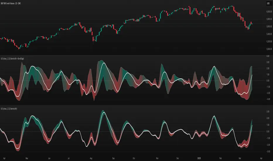
TASC 2025.04 The Ultimate Oscillator█ OVERVIEW
This script implements an alternative, refined version of the Ultimate Oscillator (UO) designed to reduce lag and enhance responsiveness in momentum indicators, as introduced by John F. Ehlers in his article "Less Lag In Momentum Indicators, The Ultimate Oscillator" from the April 2025 edition of TASC's Traders' Tips .
█ CONCEPTS
In his article, Ehlers states that indicators are essentially filters that remove unwanted noise (i.e., unnecessary information) from market data. Simply put, they process a series of data to place focus on specific information, providing a different perspective on price dynamics. Various filter types attenuate different periodic signals within the data. For instance, a lowpass filter allows only low-frequency signals, a highpass filter allows only high-frequency signals, and a bandpass filter allows signals within a specific frequency range .
Ehlers explains that the key to removing indicator lag is to combine filters of different types in such a way that the result preserves necessary, useful signals while minimizing delay (lag). His proposed UltimateOscillator aims to maintain responsiveness to a specific frequency range by measuring the difference between two highpass filters' outputs. The oscillator uses the following formula:
UO = (HP1 - HP2) / RMS
Where:
HP1 is the first highpass filter.
HP2 is another highpass filter that allows only shorter wavelengths than the critical period of HP1.
RMS is the root mean square of the highpass filter difference, used as a scaling factor to standardize the output.
The resulting oscillator is similar to a bandpass filter , because it emphasizes wavelengths between the critical periods of the two highpass filters. Ehlers' UO responds quickly to value changes in a series, providing a responsive view of momentum with little to no lag.
█ USAGE
Ehlers' UltimateOscillator sets the critical periods of its highpass filters using two parameters: BandEdge and Bandwidth :
The BandEdge sets the critical period of the second highpass filter, which determines the shortest wavelengths in the response.
The Bandwidth is a multiple of the BandEdge used for the critical period of the first highpass filter, which determines the longest wavelengths in the response. Ehlers suggests that a Bandwidth value of 2 works well for most applications. However, traders can use any value above or equal to 1.4.
Users can customize these parameters with the "Bandwidth" and "BandEdge" inputs in the "Settings/Inputs" tab.
The script plots the UO calculated for the specified "Source" series in a separate pane, with a color based on the chart's foreground color. Positive UO values indicate upward momentum or trends, and negative UO values indicate the opposite.
Additionally, this indicator provides the option to display a "cloud" from 10 additional UO series with different settings for an aggregate view of momentum. The "Cloud" input offers four display choices: "Bandwidth", "BandEdge", "Bandwidth + BandEdge", or "None".
The "Bandwidth" option calculates oscillators with different Bandwidth values based on the main oscillator's setting. Likewise, the "BandEdge" option calculates oscillators with varying BandEdge values. The "Bandwidth + BandEdge" option calculates the extra oscillators with different values for both parameters.
When a user selects any of these options, the script plots the maximum and minimum oscillator values and fills their space with a color gradient. The fill color corresponds to the net sum of each UO's sign , indicating whether most of the UOs reflect positive or negative momentum. Green hues mean most oscillators are above zero, signifying stronger upward momentum. Red hues mean most are below zero, indicating stronger downward momentum.
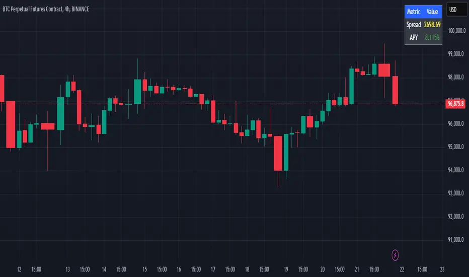
Cash And Carry Arbitrage BTC Compare Month 6 by SeoNo1Detailed Explanation of the BTC Cash and Carry Arbitrage Script
Script Title: BTC Cash And Carry Arbitrage Month 6 by SeoNo1
Short Title: BTC C&C ABT Month 6
Version: Pine Script v5
Overlay: True (The indicators are plotted directly on the price chart)
Purpose of the Script
This script is designed to help traders analyze and track arbitrage opportunities between the spot market and futures market for Bitcoin (BTC). Specifically, it calculates the spread and Annual Percentage Yield (APY) from a cash-and-carry arbitrage strategy until a specific expiry date (in this case, June 27, 2025).
The strategy helps identify profitable opportunities when the futures price of BTC is higher than the spot price. Traders can then buy BTC in the spot market and short BTC futures contracts to lock in a risk-free profit.
1. Input Settings
Spot Symbol: The real-time BTC spot price from Binance (BTCUSDT).
Futures Symbol: The BTC futures contract that expires in June 2025 (BTCUSDM2025).
Expiry Date: The expiration date of the futures contract, set to June 27, 2025.
These inputs allow users to adjust the symbols or expiry date according to their trading needs.
2. Price Data Retrieval
Spot Price: Fetches the latest closing price of BTC from the spot market.
Futures Price: Fetches the latest closing price of BTC futures.
Spread: The difference between the futures price and the spot price (futures_price - spot_price).
The spread indicates how much higher (or lower) the futures price is compared to the spot market.
3. Time to Maturity (TTM) and Annual Percentage Yield (APY) Calculation
Current Date: Gets the current timestamp.
Time to Maturity (TTM): The number of days left until the futures contract expires.
APY Calculation:
Formula:
APY = ( Spread / Spot Price ) x ( 365 / TTM Days ) x 100
This represents the annualized return from holding a cash-and-carry arbitrage position if the trader buys BTC at the spot price and sells BTC futures.
4. Display Information Table on the Chart
A table is created on the chart's top-right corner showing the following data:
Metric: Labels such as Spread and APY
Value: Displays the calculated spread and APY
The table automatically updates at the latest bar to display the most recent data.
5. Alert Condition
This sets an alert condition that triggers every time the script runs.
In practice, users can modify this alert to trigger based on specific conditions (e.g., APY exceeds a threshold).
6. Plotting the APY and Spread
APY Plot: Displays the annualized yield as a blue line on the chart.
Spread Plot: Visualizes the futures-spot spread as a red line.
This helps traders quickly identify arbitrage opportunities when the spread or APY reaches desirable levels.
How to Use the Script
Monitor Arbitrage Opportunities:
A positive spread indicates a potential cash-and-carry arbitrage opportunity.
The larger the APY, the more profitable the arbitrage opportunity could be.
Timing Trades:
Execute a buy on the BTC spot market and simultaneously sell BTC futures when the APY is attractive.
Close both positions upon futures contract expiry to realize profits.
Risk Management:
Ensure you have sufficient margin to hold both positions until expiry.
Monitor funding rates and volatility, which could affect returns.
Conclusion
This script is an essential tool for traders looking to exploit price discrepancies between the BTC spot market and futures market through a cash-and-carry arbitrage strategy. It provides real-time data on spreads, annualized returns (APY), and visual alerts, helping traders make informed decisions and maximize their profit potential.
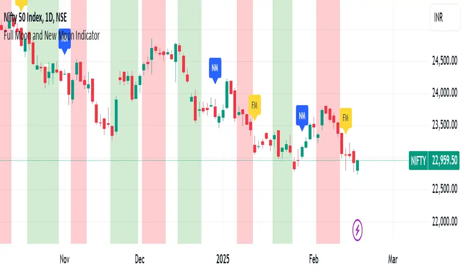
Full Moon and New Moon IndicatorThe Full Moon & New Moon Indicator is a custom Pine Script indicator which marks Full Moon (Pournami) and New Moon (Amavasya) events on the price chart. This indicator helps traders who incorporate lunar cycles into their market analysis, as certain traders believe these cycles influence market sentiment and price action. The current script is added for the year 2024 and 2025 and the dates are considered as per the Telugu calendar.
Features
✅ Identifies and labels Full Moon & New Moon days on the chart for the year 2024 and 2025
How it Works!
On a Full Moon day, it places a yellow label ("Pournami") above the corresponding candle.
On a New Moon day, it places a blue label ("Amavasya") above the corresponding candle.
Example Usage
When a Full Moon label appears, check for potential trend reversals or high volatility.
When a New Moon label appears, watch for market consolidation or a shift in sentiment.
Combine with candlestick patterns, support/resistance, or momentum indicators for a stronger trading setup.
🚀 Add this indicator to your TradingView chart and explore the market’s reaction to lunar cycles! 🌕
TASC 2025.03 A New Solution, Removing Moving Average Lag█ OVERVIEW
This script implements a novel technique for removing lag from a moving average, as introduced by John Ehlers in the "A New Solution, Removing Moving Average Lag" article featured in the March 2025 edition of TASC's Traders' Tips .
█ CONCEPTS
In his article, Ehlers explains that the average price in a time series represents a statistical estimate for a block of price values, where the estimate is positioned at the block's center on the time axis. In the case of a simple moving average (SMA), the calculation moves the analyzed block along the time axis and computes an average after each new sample. Because the average's position is at the center of each block, the SMA inherently lags behind price changes by half the data length.
As a solution to removing moving average lag, Ehlers proposes a new projected moving average (PMA) . The PMA smooths price data while maintaining responsiveness by calculating a projection of the average using the data's linear regression slope.
The slope of linear regression on a block of financial time series data can be expressed as the covariance between prices and sample points divided by the variance of the sample points. Ehlers derives the PMA by adding this slope across half the data length to the SMA, creating a first-order prediction that substantially reduces lag:
PMA = SMA + Slope * Length / 2
In addition, the article includes methods for calculating predictions of the PMA and the slope based on second-order and fourth-order differences. The formulas for these predictions are as follows:
PredictPMA = PMA + 0.5 * (Slope - Slope ) * Length
PredictSlope = 1.5 * Slope - 0.5 * Slope
Ehlers suggests that crossings between the predictions and the original values can help traders identify timely buy and sell signals.
█ USAGE
This indicator displays the SMA, PMA, and PMA prediction for a specified series in the main chart pane, and it shows the linear regression slope and prediction in a separate pane. Analyzing the difference between the PMA and SMA can help to identify trends. The differences between PMA or slope and its corresponding prediction can indicate turning points and potential trade opportunities.
The SMA plot uses the chart's foreground color, and the PMA and slope plots are blue by default. The plots of the predictions have a green or red hue to signify direction. Additionally, the indicator fills the space between the SMA and PMA with a green or red color gradient based on their differences:
Users can customize the source series, data length, and plot colors via the inputs in the "Settings/Inputs" tab.
█ NOTES FOR Pine Script® CODERS
The article's code implementation uses a loop to calculate all necessary sums for the slope and SMA calculations. Ported into Pine, the implementation is as follows:
pma(float src, int length) =>
float PMA = 0., float SMA = 0., float Slope = 0.
float Sx = 0.0 , float Sy = 0.0
float Sxx = 0.0 , float Syy = 0.0 , float Sxy = 0.0
for count = 1 to length
float src1 = src
Sx += count
Sy += src
Sxx += count * count
Syy += src1 * src1
Sxy += count * src1
Slope := -(length * Sxy - Sx * Sy) / (length * Sxx - Sx * Sx)
SMA := Sy / length
PMA := SMA + Slope * length / 2
However, loops in Pine can be computationally expensive, and the above loop's runtime scales directly with the specified length. Fortunately, Pine's built-in functions often eliminate the need for loops. This indicator implements the following function, which simplifies the process by using the ta.linreg() and ta.sma() functions to calculate equivalent slope and SMA values efficiently:
pma(float src, int length) =>
float Slope = ta.linreg(src, length, 0) - ta.linreg(src, length, 1)
float SMA = ta.sma(src, length)
float PMA = SMA + Slope * length * 0.5
To learn more about loop elimination in Pine, refer to this section of the User Manual's Profiling and optimization page.
TASC 2025.02 Autocorrelation Indicator█ OVERVIEW
This script implements the Autocorrelation Indicator introduced by John Ehlers in the "Drunkard's Walk: Theory And Measurement By Autocorrelation" article from the February 2025 edition of TASC's Traders' Tips . The indicator calculates the autocorrelation of a price series across several lags to construct a periodogram , which traders can use to identify market cycles, trends, and potential reversal patterns.
█ CONCEPTS
Drunkard's walk
A drunkard's walk , formally known as a random walk , is a type of stochastic process that models the evolution of a system or variable through successive random steps.
In his article, John Ehlers relates this model to market data. He discusses two first- and second-order partial differential equations, modified for discrete (non-continuous) data, that can represent solutions to the discrete random walk problem: the diffusion equation and the wave equation. According to Ehlers, market data takes on a mixture of two "modes" described by these equations. He theorizes that when "diffusion mode" is dominant, trading success is almost a matter of luck, and when "wave mode" is dominant, indicators may have improved performance.
Pink spectrum
John Ehlers explains that many recent academic studies affirm that market data has a pink spectrum , meaning the power spectral density of the data is proportional to the wavelengths it contains, like pink noise . A random walk with a pink spectrum suggests that the states of the random variable are correlated and not independent. In other words, the random variable exhibits long-range dependence with respect to previous states.
Autocorrelation function (ACF)
Autocorrelation measures the correlation of a time series with a delayed copy, or lag , of itself. The autocorrelation function (ACF) is a method that evaluates autocorrelation across a range of lags , which can help to identify patterns, trends, and cycles in stochastic market data. Analysts often use ACF to detect and characterize long-range dependence in a time series.
The Autocorrelation Indicator evaluates the ACF of market prices over a fixed range of lags, expressing the results as a color-coded heatmap representing a dynamic periodogram. Ehlers suggests the information from the periodogram can help traders identify different market behaviors, including:
Cycles : Distinguishable as repeated patterns in the periodogram.
Reversals : Indicated by sharp vertical changes in the periodogram when the indicator uses a short data length .
Trends : Indicated by increasing correlation across lags, starting with the shortest, over time.
█ USAGE
This script calculates the Autocorrelation Indicator on an input "Source" series, smoothed by Ehlers' UltimateSmoother filter, and plots several color-coded lines to represent the periodogram's information. Each line corresponds to an analyzed lag, with the shortest lag's line at the bottom of the pane. Green hues in the line indicate a positive correlation for the lag, red hues indicate a negative correlation (anticorrelation), and orange or yellow hues mean the correlation is near zero.
Because Pine has a limit on the number of plots for a single indicator, this script divides the periodogram display into three distinct ranges that cover different lags. To see the full periodogram, add three instances of this script to the chart and set the "Lag range" input for each to a different value, as demonstrated in the chart above.
With a modest autocorrelation length, such as 20 on a "1D" chart, traders can identify seasonal patterns in the price series, which can help to pinpoint cycles and moderate trends. For instance, on the daily ES1! chart above, the indicator shows repetitive, similar patterns through fall 2023 and winter 2023-2024. The green "triangular" shape rising from the zero lag baseline over different time ranges corresponds to seasonal trends in the data.
To identify turning points in the price series, Ehlers recommends using a short autocorrelation length, such as 2. With this length, users can observe sharp, sudden shifts along the vertical axis, which suggest potential turning points from upward to downward or vice versa.

Highs & Lows RTH/OVN/IBs/D/W/M/YOverview
Plots the highs and lows of RTH, OVN/ETH, IBs of those sessions, previous Day, Week, Month, and Year.
Features
Allows the user to enable/disable plotting the high/low of each period.
Lines' length, offset, and colors can be customized
Labels' position, size, color, and style can be customized
Support
Questions, feedbacks, and requests are welcomed. Please feel free to use Comments or direct private message via TradingView.
Disclaimer
This stock chart indicator provided is for informational purposes only and should not be considered as financial or investment advice. The data and information presented in this indicator are obtained from sources believed to be reliable, but we do not warrant its completeness or accuracy.
Users should be aware that:
Any investment decisions made based on this indicator are at your own risk.
The creators and providers of this indicator disclaim all liability for any losses, damages, or other consequences resulting from its use. By using this stock chart indicator, you acknowledge and accept the inherent risks associated with trading and investing in financial markets.
Release Date: 2025-01-17
Release Version: v1 r1
Release Notes Date: 2025-01-17

TASC 2025.01 Linear Predictive Filters█ OVERVIEW
This script implements a suite of tools for identifying and utilizing dominant cycles in time series data, as introduced by John Ehlers in the "Linear Predictive Filters And Instantaneous Frequency" article featured in the January 2025 edition of TASC's Traders' Tips . Dominant cycle information can help traders adapt their indicators and strategies to changing market conditions.
█ CONCEPTS
Conventional technical indicators and strategies often rely on static, unchanging parameters, which may fail to account for the dynamic nature of market data. In his article, John Ehlers applies digital signal processing principles to address this issue, introducing linear predictive filters to identify cyclic information for adapting indicators and strategies to evolving market conditions.
This approach treats market data as a complex series in the time domain. Analyzing the series in the frequency domain reveals information about its cyclic components. To reduce the impact of frequencies outside a range of interest and focus on a specific range of cycles, Ehlers applies second-order highpass and lowpass filters to the price data, which attenuate or remove wavelengths outside the desired range. This band-limited analysis isolates specific parts of the frequency spectrum for various trading styles, e.g., longer wavelengths for position trading or shorter wavelengths for swing trading.
After filtering the series to produce band-limited data, Ehlers applies a linear predictive filter to predict future values a few bars ahead. The filter, calculated based on the techniques proposed by Lloyd Griffiths, adaptively minimizes the error between the latest data point and prediction, successively adjusting its coefficients to align with the band-limited series. The filter's coefficients can then be applied to generate an adaptive estimate of the band-limited data's structure in the frequency domain and identify the dominant cycle.
█ USAGE
This script implements the following tools presented in the article:
Griffiths Predictor
This tool calculates a linear predictive filter to forecast future data points in band-limited price data. The crosses between the prediction and signal lines can provide potential trade signals.
Griffiths Spectrum
This tool calculates a partial frequency spectrum of the band-limited price data derived from the linear predictive filter's coefficients, displaying a color-coded representation of the frequency information in the pane. This mode's display represents the data as a periodogram . The bottom of each plotted bar corresponds to a specific analyzed period (inverse of frequency), and the bar's color represents the presence of that periodic cycle in the time series relative to the one with the highest presence (i.e., the dominant cycle). Warmer, brighter colors indicate a higher presence of the cycle in the series, whereas darker colors indicate a lower presence.
Griffiths Dominant Cycle
This tool compares the cyclic components within the partial spectrum and identifies the frequency with the highest power, i.e., the dominant cycle . Traders can use this dominant cycle information to tune other indicators and strategies, which may help promote better alignment with dynamic market conditions.
Notes on parameters
Bandpass boundaries:
In the article, Ehlers recommends an upper bound of 125 bars or higher to capture longer-term cycles for position trading. He recommends an upper bound of 40 bars and a lower bound of 18 bars for swing trading. If traders use smaller lower bounds, Ehlers advises a minimum of eight bars to minimize the potential effects of aliasing.
Data length:
The Griffiths predictor can use a relatively small data length, as autocorrelation diminishes rapidly with lag. However, for optimal spectrum and dominant cycle calculations, the length must match or exceed the upper bound of the bandpass filter. Ehlers recommends avoiding excessively long lengths to maintain responsiveness to shorter-term cycles.

Ripple (XRP) Model PriceAn article titled Bitcoin Stock-to-Flow Model was published in March 2019 by "PlanB" with mathematical model used to calculate Bitcoin model price during the time. We know that Ripple has a strong correlation with Bitcoin. But does this correlation have a definite rule?
In this study, we examine the relationship between bitcoin's stock-to-flow ratio and the ripple(XRP) price.
The Halving and the stock-to-flow ratio
Stock-to-flow is defined as a relationship between production and current stock that is out there.
SF = stock / flow
The term "halving" as it relates to Bitcoin has to do with how many Bitcoin tokens are found in a newly created block. Back in 2009, when Bitcoin launched, each block contained 50 BTC, but this amount was set to be reduced by 50% every 210,000 blocks (about 4 years). Today, there have been three halving events, and a block now only contains 6.25 BTC. When the next halving occurs, a block will only contain 3.125 BTC. Halving events will continue until the reward for minors reaches 0 BTC.
With each halving, the stock-to-flow ratio increased and Bitcoin experienced a huge bull market that absolutely crushed its previous all-time high. But what exactly does this affect the price of Ripple?
Price Model
I have used Bitcoin's stock-to-flow ratio and Ripple's price data from April 1, 2014 to November 3, 2021 (Daily Close-Price) as the statistical population.
Then I used linear regression to determine the relationship between the natural logarithm of the Ripple price and the natural logarithm of the Bitcoin's stock-to-flow (BSF).
You can see the results in the image below:
Basic Equation : ln(Model Price) = 3.2977 * ln(BSF) - 12.13
The high R-Squared value (R2 = 0.83) indicates a large positive linear association.
Then I "winsorized" the statistical data to limit extreme values to reduce the effect of possibly spurious outliers (This process affected less than 4.5% of the total price data).
ln(Model Price) = 3.3297 * ln(BSF) - 12.214
If we raise the both sides of the equation to the power of e, we will have:
============================================
Final Equation:
■ Model Price = Exp(- 12.214) * BSF ^ 3.3297
Where BSF is Bitcoin's stock-to-flow
============================================
If we put current Bitcoin's stock-to-flow value (54.2) into this equation we get value of 2.95USD. This is the price which is indicated by the model.
There is a power law relationship between the market price and Bitcoin's stock-to-flow (BSF). Power laws are interesting because they reveal an underlying regularity in the properties of seemingly random complex systems.
I plotted XRP model price (black) over time on the chart.
Estimating the range of price movements
I also used several bands to estimate the range of price movements and used the residual standard deviation to determine the equation for those bands.
Residual STDEV = 0.82188
ln(First-Upper-Band) = 3.3297 * ln(BSF) - 12.214 + Residual STDEV =>
ln(First-Upper-Band) = 3.3297 * ln(BSF) – 11.392 =>
■ First-Upper-Band = Exp(-11.392) * BSF ^ 3.3297
In the same way:
■ First-Lower-Band = Exp(-13.036) * BSF ^ 3.3297
I also used twice the residual standard deviation to define two extra bands:
■ Second-Upper-Band = Exp(-10.570) * BSF ^ 3.3297
■ Second-Lower-Band = Exp(-13.858) * BSF ^ 3.3297
These bands can be used to determine overbought and oversold levels.
Estimating of the future price movements
Because we know that every four years the stock-to-flow ratio, or current circulation relative to new supply, doubles, this metric can be plotted into the future.
At the time of the next halving event, Bitcoins will be produced at a rate of 450 BTC / day. There will be around 19,900,000 coins in circulation by August 2025
It is estimated that during first year of Bitcoin (2009) Satoshi Nakamoto (Bitcoin creator) mined around 1 million Bitcoins and did not move them until today. It can be debated if those coins might be lost or Satoshi is just waiting still to sell them but the fact is that they are not moving at all ever since. We simply decrease stock amount for 1 million BTC so stock to flow value would be:
BSF = (19,900,000 – 1.000.000) / (450 * 365) =115.07
Thus, Bitcoin's stock-to-flow will increase to around 115 until AUG 2025. If we put this number in the equation:
Model Price = Exp(- 12.214) * 114 ^ 3.3297 = 36.06$
Ripple has a fixed supply rate. In AUG 2025, the total number of coins in circulation will be about 56,000,000,000. According to the equation, Ripple's market cap will reach $2 trillion.
Note that these studies have been conducted only to better understand price movements and are not a financial advice.

LDR 2025 — DayTHIS IS NOT AN INDICATOR!
It's a loving gentle reminder for traders to keep an eye if this LDR day might impact your trading.

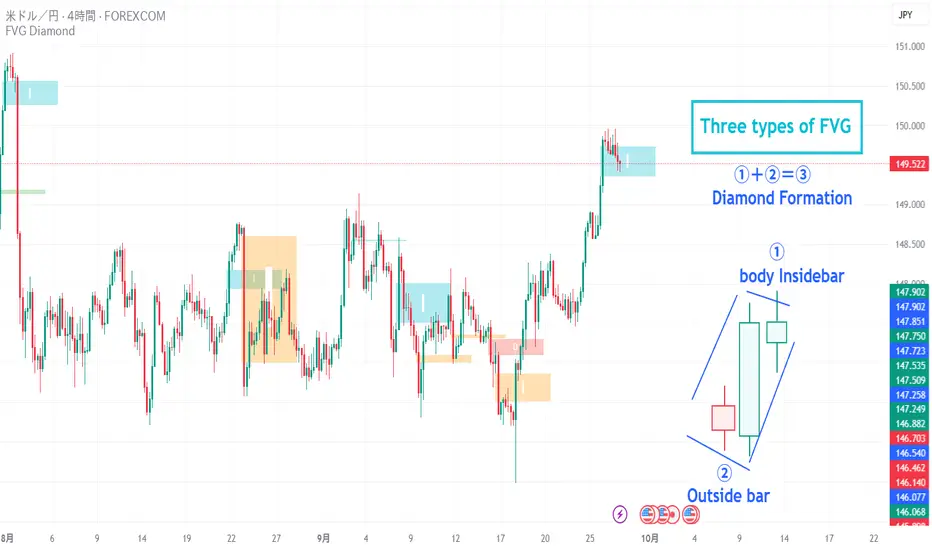
FVG Diamond📊 Overview
FVG Diamond is an advanced indicator that detects three specific price action patterns: Inside Bar, Outside Bar, and Diamond Formation. Unlike basic FVG tools, it focuses on these higher-level setups for more precise analysis.
✨ Key Features
🎯 Detection of 3 Advanced FVG Pattern Types
Independent on/off toggle for each pattern
Inside FVG (Inside Bar / Harami): The body of the 3rd candle forms an inside bar relative to the 2nd candle
Outside FVG (Outside Bar / Engulfing): The body of the 1st candle forms an outside bar relative to the 2nd candle
Diamond FVG (Diamond Formation): A unique pattern that satisfies both Inside and Outside conditions
🎯 Mitigation Feature
ON: FVG boxes are automatically removed once price fully fills the FVG zone (keeps the chart clean by showing only active FVGs)
OFF: FVG boxes remain on the chart indefinitely (allows full historical review of all FVGs)
🎨 Visual Features
Color Coding: Assign unique colors to each pattern type
Transparency Control: Default 70% transparency for optimal readability
Extension Display: Extend the right edge of FVG boxes for any number of bars
⚙️ Advanced Configuration
Threshold Settings
Manual Threshold: Define a minimum gap size by percentage
Auto Threshold: Dynamically adjusts based on market volatility
Mitigation Tools
Real-Time Mitigation: Automatic removal when price fills an FVG zone
Mitigation Levels: Display filled FVG levels with dashed lines
🔔 Alerts
Notification on new Bullish/Bearish FVG detection
Notification when an FVG is mitigated (filled)
Works with all FVG types
📈 How to Use
Add the indicator to your chart
The three advanced FVG patterns will be detected and displayed automatically
Set your preferred threshold (0% = detect all gaps)
⚠️ Note: This indicator is designed as an analysis support tool. Trading decisions should be made in combination with other methods of technical and fundamental analysis.
Author: omochi_
Version: 1.0
Last Updated: September 28, 2025
Macro & Earnings Dashboard — NY Fed CalendarMacro & Earnings Dashboard — NY Fed Calendar
This is an overlay indicator designed to provide a quick, real-time overview of the most critical upcoming US economic data releases and corporate earnings reports directly on your TradingView chart. It functions as a dynamic dashboard, removing the need to constantly check external calendars.
Key Features
1. Real-Time Economic Calendar (Bottom-Right Table)
The dashboard tracks the time remaining until the next release of five major, high-impact economic indicators. The data for these dates is pre-loaded directly from the New York Fed Economic Indicators Calendar (currently loaded for October through December 2025).
The tracked events include:
CPI (Consumer Price Index)
PPI (Producer Price Index)
Employment Situation (Non-Farm Payrolls / Unemployment Rate)
Interest Rate Decision (FOMC Meetings)
Consumer Sentiment (University of Michigan Survey)
2. Corporate Earnings Tracker (Top-Right Table)
This table uses TradingView's built-in data to calculate the estimated days remaining until the next Earnings Per Share (EPS) report for a curated list of high-profile NASDAQ tickers:
AAPL, NVDA, GOOG, TSLA, MSFT, AMZN, META
3. Color-Coded Urgency
The "Days" column for both macro and earnings tables uses a traffic light system to instantly communicate how soon the event is:
Red: The event is scheduled for Today or Tomorrow (0–1 day away).
Orange: The event is scheduled for the current week (within 6 days).
Teal: The event is more than a week away.
Gray: The date is currently unavailable or outside the loaded calendar range.

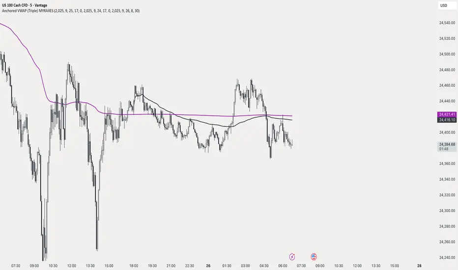
Anchored VWAP (Triple) MYRAXESAnchored VWAP Triple Indicator
The Anchored VWAP Triple indicator is a powerful tool for technical analysis, allowing traders to plot three customizable anchored Volume Weighted Average Price (VWAP) lines on a chart. Unlike traditional VWAP, which resets daily, this indicator lets you anchor each VWAP to a specific date and time, providing a unique perspective on price action relative to key market events.
Features
Three Independent VWAPs: Plot up to three VWAP lines, each anchored to a user-defined date and time.
Customizable Inputs: Set the year, month, day, hour, and minute for each VWAP anchor point. Choose distinct colors for easy identification.
Pure Anchored Design: VWAP lines start only from the anchor point, with no pre-anchor extensions, ensuring a clean and focused analysis.
Debug Mode: Optional display of hour and minute for troubleshooting or educational purposes.
Default Settings: Pre-configured with practical defaults (e.g., September 2025 dates) for immediate use.
How to Use
Add the indicator to your TradingView chart.
Adjust the anchor dates and times for each VWAP (VWAP 1, VWAP 2, VWAP 3) via the input settings.
Select custom colors for each VWAP line to differentiate them on the chart.
Enable Debug Mode if needed to verify time alignment.
Analyze price movements relative to the anchored VWAPs to identify support, resistance, or trend shifts.
Benefits
Ideal for swing traders and long-term analysts who need to anchor VWAP to significant price levels or events.
Enhances decision-making by comparing multiple VWAPs from different anchor points.
Fully compatible with TradingView’s Pine Script v6 for smooth performance.
This indicator is perfect for traders looking to deepen their market analysis with a flexible, multi-VWAP approach. Share your feedback or custom setups in the comments!
CB Charts - GEX MESZ2025/ESZ2025Last Updated: 09/22/2025 6:41 a.m. PST
*DISCLAIMER: Only intended for ESZ2025/MESZ2025 charts.
This indicator plots horizontal levels based on batched GEX levels for ESZ2025/MESZ2025. The batched data is derived from contracts expiring: 0DTE, 1DTE, EoW, EoM, Next Week, Next Month and 3-months out. Labels are available for a high-level view of which levels are which. Hovering (or long-pressing on mobile TV) over the labels will display the nominal values and Rank. This script is manually updated and may not be always updated.
When and what to use:
- Most respected levels come from 1DTE, EoW and EoM.
- 0DTE is included for when this script becomes intraday updated. (CURRENTLY NOT UPDATED INTRADAY)
- Next Week setting is best used only for Friday and Sunday trading
- Next Month setting is best for weeks close to the end of the current month
Powered by the Camels of Wallstreet

Japan Yen Carry Trade to Risk Ratio Sharpe Ratio By UncleBFMStep-by-Step Calculation in the ScriptFetch Rates:Pulls rates dynamically using request.security() from user-specified symbols (e.g., TVC:JP10Y for yen, TVC:US10Y for target). If unavailable (NA), uses fallback inputs (e.g., 0.25% for yen, 4.50% for target).
Converts rates to decimals: (target_rate - yen_rate) / 100.
Calculate Carry:Carry = (Target Rate - Yen Rate) / 100
Example: If US 10Y yield is 4.50% and Japan 10Y is 0.25%, carry = (4.50 - 0.25) / 100 = 0.0425 (4.25% annual yield).
Calculate Daily Log Returns:Log Returns = ln(Close / Close ), where Close is the current price of the pair (e.g., USDJPY) and Close is the previous day's price.
This measures daily percentage changes in a way suitable for volatility calculations.
Calculate Annualized Volatility:Volatility = Standard Deviation of Log Returns over a lookback period (default 63 days, ~3 months) × √252.
Example: If the standard deviation of USDJPY log returns is 0.005 (0.5% daily), annualized volatility = 0.005 × √252 ≈ 0.0794 (7.94%).
Compute the Ratio:Ratio = Carry / Volatility
Example: Using above, 0.0425 / 0.0794 ≈ 0.535.
If volatility is zero, the ratio is set to NA to avoid division errors.
Plot:Plots the ratio as a line, with optional thresholds (e.g., 0.2 for "high attractiveness") to guide interpretation.
NotesDynamic Rates: Using bond yields (e.g., TVC:JP10Y) or policy rates (e.g., ECONOMICS:JPINTR) makes the indicator responsive to historical and current rate changes, unlike static inputs.
Context: BIS reports use similar ratios to assess carry trade viability. For USDJPY in 2025, with Fed rates around 4.5% and BoJ at 0.25–0.5%, the carry is positive but sensitive to volatility spikes (e.g., during 2024 unwind events).
Usage: Apply to a yen pair chart (e.g., USDJPY, AUDJPY). Adjust symbols for the target currency (e.g., TVC:AU10Y for AUD). The ratio helps compare carry trade profitability across pairs or over time.
