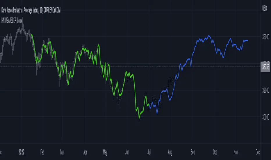
Helme-Nikias Weighted Burg AR-SE Extra. of Price [Loxx]Helme-Nikias Weighted Burg AR-SE Extra. of Price is an indicator that uses an autoregressive spectral estimation called the Weighted Burg Algorithm, but unlike the usual WB algo, this one uses Helme-Nikias weighting. This method is commonly used in speech modeling and speech prediction engines. This is a linear method of forecasting data. You'll notice that this method uses a different weighting calculation vs Weighted Burg method. This new weighting is the following:
w = math.pow(array.get(x, i - 1), 2), the squared lag of the source parameter
and
w += math.pow(array.get(x, i), 2), the sum of the squared source parameter
This take place of the rectangular, hamming and parabolic weighting used in the Weighted Burg method
Also, this method includes Levinson–Durbin algorithm. as was already discussed previously in the following indicator:
Levinson-Durbin Autocorrelation Extrapolation of Price
What is Helme-Nikias Weighted Burg Autoregressive Spectral Estimate Extrapolation of price?
In this paper a new stable modification of the weighted Burg technique for autoregressive (AR) spectral estimation is introduced based on data-adaptive weights that are proportional to the common power of the forward and backward AR process realizations. It is shown that AR spectra of short length sinusoidal signals generated by the new approach do not exhibit phase dependence or line-splitting. Further, it is demonstrated that improvements in resolution may be so obtained relative to other weighted Burg algorithms. The method suggested here is shown to resolve two closely-spaced peaks of dynamic range 24 dB whereas the modified Burg schemes employing rectangular, Hamming or "optimum" parabolic windows fail.
Data inputs
Source Settings: -Loxx's Expanded Source Types. You typically use "open" since open has already closed on the current active bar
LastBar - bar where to start the prediction
PastBars - how many bars back to model
LPOrder - order of linear prediction model; 0 to 1
FutBars - how many bars you want to forward predict
Things to know
Normally, a simple moving average is calculated on source data. I've expanded this to 38 different averaging methods using Loxx's Moving Avreages.
This indicator repaints
Further reading
A high-resolution modified Burg algorithm for spectral estimation
Related Indicators
Levinson-Durbin Autocorrelation Extrapolation of Price
Weighted Burg AR Spectral Estimate Extrapolation of Price
Cari skrip untuk "wind+芯片行业+市盈率+财经数据"
[blackcat] L1 Vitali Apirine HHs & LLs StochasticsLevel 1
Background
This indicator was originally formulated by Vitali Apirine for TASC - February 2016 Traders Tips.
Function
According to Vitali Apirine, his momentum indicator–based system HHLLS (higher high lower low stochastic) can help to spot emerging trends, define correction periods, and anticipate reversals. As with many indicators, HHLLS signals can also be generated by looking for divergences and crossovers. Because the HHLLS is an oscillator, it can also be used to identify overbought & oversold levels.
Remarks
I changed EMA or SMA into hanning windowing function to reduce lag issue.
colorful area is bearish power.
colorful solid thick line is bull power.
Feedbacks are appreciated.

No Climactic BarsThis script can be used to detect large candles, similiar to ATR, using the variance of a sliding windows and certain threshold.

NormalizedOscillatorsLibrary "NormalizedOscillators"
Collection of some common Oscillators. All are zero-mean and normalized to fit in the -1..1 range. Some are modified, so that the internal smoothing function could be configurable (for example, to enable Hann Windowing, that John F. Ehlers uses frequently). Some are modified for other reasons (see comments in the code), but never without a reason. This collection is neither encyclopaedic, nor reference, however I try to find the most correct implementation. Suggestions are welcome.
rsi2(upper, lower) RSI - second step
Parameters:
upper : Upwards momentum
lower : Downwards momentum
Returns: Oscillator value
Modified by Ehlers from Wilder's implementation to have a zero mean (oscillator from -1 to +1)
Originally: 100.0 - (100.0 / (1.0 + upper / lower))
Ignoring the 100 scale factor, we get: upper / (upper + lower)
Multiplying by two and subtracting 1, we get: (2 * upper) / (upper + lower) - 1 = (upper - lower) / (upper + lower)
rms(src, len) Root mean square (RMS)
Parameters:
src : Source series
len : Lookback period
Based on by John F. Ehlers implementation
ift(src) Inverse Fisher Transform
Parameters:
src : Source series
Returns: Normalized series
Based on by John F. Ehlers implementation
The input values have been multiplied by 2 (was "2*src", now "4*src") to force expansion - not compression
The inputs may be further modified, if needed
stoch(src, len) Stochastic
Parameters:
src : Source series
len : Lookback period
Returns: Oscillator series
ssstoch(src, len) Super Smooth Stochastic (part of MESA Stochastic) by John F. Ehlers
Parameters:
src : Source series
len : Lookback period
Returns: Oscillator series
Introduced in the January 2014 issue of Stocks and Commodities
This is not an implementation of MESA Stochastic, as it is based on Highpass filter not present in the function (but you can construct it)
This implementation is scaled by 0.95, so that Super Smoother does not exceed 1/-1
I do not know, if this the right way to fix this issue, but it works for now
netKendall(src, len) Noise Elimination Technology by John F. Ehlers
Parameters:
src : Source series
len : Lookback period
Returns: Oscillator series
Introduced in the December 2020 issue of Stocks and Commodities
Uses simplified Kendall correlation algorithm
Implementation by @QuantTherapy:
rsi(src, len, smooth) RSI
Parameters:
src : Source series
len : Lookback period
smooth : Internal smoothing algorithm
Returns: Oscillator series
vrsi(src, len, smooth) Volume-scaled RSI
Parameters:
src : Source series
len : Lookback period
smooth : Internal smoothing algorithm
Returns: Oscillator series
This is my own version of RSI. It scales price movements by the proportion of RMS of volume
mrsi(src, len, smooth) Momentum RSI
Parameters:
src : Source series
len : Lookback period
smooth : Internal smoothing algorithm
Returns: Oscillator series
Inspired by RocketRSI by John F. Ehlers (Stocks and Commodities, May 2018)
rrsi(src, len, smooth) Rocket RSI
Parameters:
src : Source series
len : Lookback period
smooth : Internal smoothing algorithm
Returns: Oscillator series
Inspired by RocketRSI by John F. Ehlers (Stocks and Commodities, May 2018)
Does not include Fisher Transform of the original implementation, as the output must be normalized
Does not include momentum smoothing length configuration, so always assumes half the lookback length
mfi(src, len, smooth) Money Flow Index
Parameters:
src : Source series
len : Lookback period
smooth : Internal smoothing algorithm
Returns: Oscillator series
lrsi(src, in_gamma, len) Laguerre RSI by John F. Ehlers
Parameters:
src : Source series
in_gamma : Damping factor (default is -1 to generate from len)
len : Lookback period (alternatively, if gamma is not set)
Returns: Oscillator series
The original implementation is with gamma. As it is impossible to collect gamma in my system, where the only user input is length,
an alternative calculation is included, where gamma is set by dividing len by 30. Maybe different calculation would be better?
fe(len) Choppiness Index or Fractal Energy
Parameters:
len : Lookback period
Returns: Oscillator series
The Choppiness Index (CHOP) was created by E. W. Dreiss
This indicator is sometimes called Fractal Energy
er(src, len) Efficiency ratio
Parameters:
src : Source series
len : Lookback period
Returns: Oscillator series
Based on Kaufman Adaptive Moving Average calculation
This is the correct Efficiency ratio calculation, and most other implementations are wrong:
the number of bar differences is 1 less than the length, otherwise we are adding the change outside of the measured range!
For reference, see Stocks and Commodities June 1995
dmi(len, smooth) Directional Movement Index
Parameters:
len : Lookback period
smooth : Internal smoothing algorithm
Returns: Oscillator series
Based on the original Tradingview algorithm
Modified with inspiration from John F. Ehlers DMH (but not implementing the DMH algorithm!)
Only ADX is returned
Rescaled to fit -1 to +1
Unlike most oscillators, there is no src parameter as DMI works directly with high and low values
fdmi(len, smooth) Fast Directional Movement Index
Parameters:
len : Lookback period
smooth : Internal smoothing algorithm
Returns: Oscillator series
Same as DMI, but without secondary smoothing. Can be smoothed later. Instead, +DM and -DM smoothing can be configured
doOsc(type, src, len, smooth) Execute a particular Oscillator from the list
Parameters:
type : Oscillator type to use
src : Source series
len : Lookback period
smooth : Internal smoothing algorithm
Returns: Oscillator series
Chande Momentum Oscillator (CMO) is RSI without smoothing. No idea, why some authors use different calculations
LRSI with Fractal Energy is a combo oscillator that uses Fractal Energy to tune LRSI gamma, as seen here: www.prorealcode.com
doPostfilter(type, src, len) Execute a particular Oscillator Postfilter from the list
Parameters:
type : Oscillator type to use
src : Source series
len : Lookback period
Returns: Oscillator series

Directional Movement w/Hann Slope Change SignalModified version of
Presented here is code for the "Directional Movement w/Hann" indicator originally conceived by John Ehlers. The code is also published in the December 2021 issue of Trader's Tips by Technical Analysis of Stocks & Commodities (TASC) magazine.
John Ehlers is continuing to revamp old indictors with Hann windowing. The original script uses zero line cross to signal buy/sell in this modified version buy/sell is signaled based on slope change, where signal is generated on with previous value is greater/less than current value
If current > previous = buy and if current < previous = sell

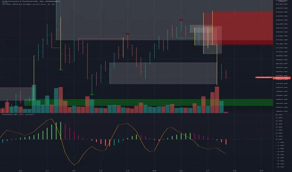
MAD indicator Enchanced (MADH, inspired by J.Ehlers)This oscillator was inspired by the recent J. Ehler's article (Stocks & Commodities V. 39:11 (24–26): The MAD Indicator, Enhanced by John F. Ehlers). Basically, it shows the difference between two move averages, an "enhancement" made by the author in the last version comes down to replacement SMA to a weighted average that uses Hann windowing. I took the liberty to add colors, ROC line (well, you know, no shorts when ROC's negative and no long's when positive, etc), and optional usage of PVT (price-volume trend) as the source (instead of just price).
[blackcat] L2 Ehlers Adaptive Jon Andersen R-Squared IndicatorLevel: 2
Background
@pips_v1 has proposed an interesting idea that is it possible to code an "Adaptive Jon Andersen R-Squared Indicator" where the length is determined by DCPeriod as calculated in Ehlers Sine Wave Indicator? I agree with him and starting to construct this indicator. After a study, I found "(blackcat) L2 Ehlers Autocorrelation Periodogram" script could be reused for this purpose because Ehlers Autocorrelation Periodogram is an ideal candidate to calculate the dominant cycle. On the other hand, there are two inputs for R-Squared indicator:
Length - number of bars to calculate moment correlation coefficient R
AvgLen - number of bars to calculate average R-square
I used Ehlers Autocorrelation Periodogram to produced a dynamic value of "Length" of R-Squared indicator and make it adaptive.
Function
One tool available in forecasting the trendiness of the breakout is the coefficient of determination (R-squared), a statistical measurement. The R-squared indicates linear strength between the security's price (the Y - axis) and time (the X - axis). The R-squared is the percentage of squared error that the linear regression can eliminate if it were used as the predictor instead of the mean value. If the R-squared were 0.99, then the linear regression would eliminate 99% of the error for prediction versus predicting closing prices using a simple moving average.
When the R-squared is at an extreme low, indicating that the mean is a better predictor than regression, it can only increase, indicating that the regression is becoming a better predictor than the mean. The opposite is true for extreme high values of the R-squared.
To make this indicator adaptive, the dominant cycle is extracted from the spectral estimate in the next block of code using a center-of-gravity ( CG ) algorithm. The CG algorithm measures the average center of two-dimensional objects. The algorithm computes the average period at which the powers are centered. That is the dominant cycle. The dominant cycle is a value that varies with time. The spectrum values vary between 0 and 1 after being normalized. These values are converted to colors. When the spectrum is greater than 0.5, the colors combine red and yellow, with yellow being the result when spectrum = 1 and red being the result when the spectrum = 0.5. When the spectrum is less than 0.5, the red saturation is decreased, with the result the color is black when spectrum = 0.
Construction of the autocorrelation periodogram starts with the autocorrelation function using the minimum three bars of averaging. The cyclic information is extracted using a discrete Fourier transform (DFT) of the autocorrelation results. This approach has at least four distinct advantages over other spectral estimation techniques. These are:
1. Rapid response. The spectral estimates start to form within a half-cycle period of their initiation.
2. Relative cyclic power as a function of time is estimated. The autocorrelation at all cycle periods can be low if there are no cycles present, for example, during a trend. Previous works treated the maximum cycle amplitude at each time bar equally.
3. The autocorrelation is constrained to be between minus one and plus one regardless of the period of the measured cycle period. This obviates the need to compensate for Spectral Dilation of the cycle amplitude as a function of the cycle period.
4. The resolution of the cyclic measurement is inherently high and is independent of any windowing function of the price data.
Key Signal
DC --> Ehlers dominant cycle.
AvgSqrR --> R-squared output of the indicator.
Remarks
This is a Level 2 free and open source indicator.
Feedbacks are appreciated.

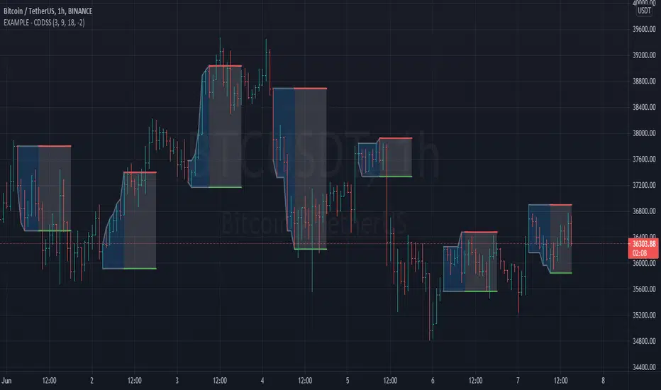
Example - Custom Defined Dual-State SessionThis script example aims to cover the following:
defining custom timeframe / session windows
gather a price range from the custom period ( high/low values )
create a secondary "holding" period through which to display the data collected from the initial session
simple method to shift times to re-align to preferred timezone
Articles and further reading:
www.investopedia.com - trading session
Reason for Study:
Educational purposes only.
Before considering writing this example I had seen multiple similar questions
asking how to go about creating custom timeframes or sessions, so it seemed
this might be a good topic to attempt to create a relatively generic example.
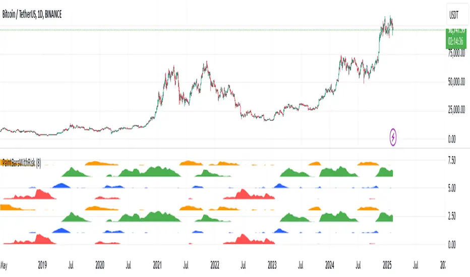
Pragmatic risk managementINTRO
The indicator is calculating multiple moving averages on the value of price change %. It then combines the normalized (via arctan function) values into a single normalized value (via simple average).
The total error from the center of gravity and the angle in which the error is accumulating represented by 4 waves:
BLUE = Good for chance for price to go up
GREEN = Good chance for price to continue going up
ORANGE = Good chance for price to go down
RED = Good chance for price to continue going down
A full cycle of ORANGE\RED\BLUE\GREEN colors will ideally lead to the exact same cycle, if not, try to understand why.
NOTICE-
This indicator is calculating large time-windows so It can be heavy on your device. Tested on PC browser only.
My visual setup:
1. Add two indicators on-top of each other and merge their scales (It will help out later).
2. Zoom out price chart to see the maximum possible data.
3. Set different colors for both indicators for simple visual seperation.
4. Choose 2 different values, one as high as possible and one as low as possible.
(Possible - the indicator remains effective at distinguishing the cycle).
Manual calibration:
0. Select a fixed chart resolution (2H resolution minimum recommended).
1. Change the "mul2" parameter in ranges between 4-15 .
2. Observe the "Turning points" of price movement. (Typically when RED\GREEN are about to switch.)
2. Perform a segmentation of time slices and find cycles. No need to be exact!
3. Draw a square on price movement at place and color as the dominant wave currently inside the indicator.
This procedure should lead to a full price segmentation with easier anchoring.
[blackcat] L2 Ehlers Autocorrelation PeriodogramLevel: 2
Background
John F. Ehlers introduced Autocorrelation Periodogram in his "Cycle Analytics for Traders" chapter 8 on 2013.
Function
Construction of the autocorrelation periodogram starts with the autocorrelation function using the minimum three bars of averaging. The cyclic information is extracted using a discrete Fourier transform (DFT) of the autocorrelation results. This approach has at least four distinct advantages over other spectral estimation techniques. These are:
1. Rapid response. The spectral estimates start to form within a half-cycle period of their initiation.
2. Relative cyclic power as a function of time is estimated. The autocorrelation at all cycle periods can be low if there are no cycles present, for example, during a trend. Previous works treated the maximum cycle amplitude at each time bar equally.
3. The autocorrelation is constrained to be between minus one and plus one regardless of the period of the measured cycle period. This obviates the need to compensate for Spectral Dilation of the cycle amplitude as a function of the cycle period.
4. The resolution of the cyclic measurement is inherently high and is independent of any windowing function of the price data.
The dominant cycle is extracted from the spectral estimate in the next block of code using a center-of-gravity (CG) algorithm. The CG algorithm measures the average center of two-dimensional objects. The algorithm computes the average period at which the powers are centered. That is the dominant cycle. The dominant cycle is a value that varies with time. The spectrum values vary between 0 and 1 after being normalized. These values are converted to colors. When the spectrum is greater than 0.5, the colors combine red and yellow, with yellow being the result when spectrum = 1 and red being the result when the spectrum = 0.5. When the spectrum is less than 0.5, the red saturation is decreased, with the result the color is black when spectrum = 0.
Key Signal
DominantCycle --> Dominant Cycle
Period --> Autocorrelation Periodogram Array
Pros and Cons
100% John F. Ehlers definition translation of original work, even variable names are the same. This help readers who would like to use pine to read his book. If you had read his works, then you will be quite familiar with my code style.
Remarks
The 49th script for Blackcat1402 John F. Ehlers Week publication.
Courtesy of @RicardoSantos for RGB functions.
Readme
In real life, I am a prolific inventor. I have successfully applied for more than 60 international and regional patents in the past 12 years. But in the past two years or so, I have tried to transfer my creativity to the development of trading strategies. Tradingview is the ideal platform for me. I am selecting and contributing some of the hundreds of scripts to publish in Tradingview community. Welcome everyone to interact with me to discuss these interesting pine scripts.
The scripts posted are categorized into 5 levels according to my efforts or manhours put into these works.
Level 1 : interesting script snippets or distinctive improvement from classic indicators or strategy. Level 1 scripts can usually appear in more complex indicators as a function module or element.
Level 2 : composite indicator/strategy. By selecting or combining several independent or dependent functions or sub indicators in proper way, the composite script exhibits a resonance phenomenon which can filter out noise or fake trading signal to enhance trading confidence level.
Level 3 : comprehensive indicator/strategy. They are simple trading systems based on my strategies. They are commonly containing several or all of entry signal, close signal, stop loss, take profit, re-entry, risk management, and position sizing techniques. Even some interesting fundamental and mass psychological aspects are incorporated.
Level 4 : script snippets or functions that do not disclose source code. Interesting element that can reveal market laws and work as raw material for indicators and strategies. If you find Level 1~2 scripts are helpful, Level 4 is a private version that took me far more efforts to develop.
Level 5 : indicator/strategy that do not disclose source code. private version of Level 3 script with my accumulated script processing skills or a large number of custom functions. I had a private function library built in past two years. Level 5 scripts use many of them to achieve private trading strategy.

predict lagUse the angle of multiple moving time windows to calculate the angular momentum vector across time. represent in a spectrum of frequencies\colors\transparency together with the accumulative "truth" (black)

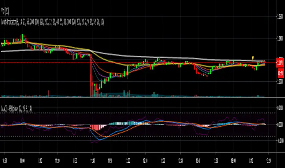
MACD + RSI togetheryou will have both MACD and RSI together in front of each other. best for tile windows or small monitors. enjoy
Better Bollinger Bands (now open source)General purpose Bollinger band indicator with a number of configuration options and some additional color-coded information. The main advantages of it over standard Bollinger bands are:
1) Better statistics:
* Uses volume weighted moving averages, variance, and standard deviation by default. The volume dependence can be disabled with a checkbox option, but generally makes it more responsive improves its ability to distinguish true outlier events from random variation.
* Lets you pick between different time windows (simple, sawtooth (WMA), exponential) in addition to the volume weighting, with appropriate Bessel corrections to make the estimators unbiased and to get consistent result for different weights.
* Has a checkbox option to use a linear regression in the band calculation if you don't want average momentum to be counted in the volatility. This turns the centerline into a last squares moving average, and the band width at each time step is given by the variance away from the regression line instead of from a moving average. Weights in the least squares regression are changed according to the other options. For tickers with a strong long-term trend this makes the bands track the price action more closely.
2) Geometric
* This does all calculations on log(price) instead of the prices themselves.
* Makes almost no difference in most cases, but gives better results on charts with strongly exponential behaviour that range between several orders of magnitude.
* Properly centered around price action on log plots.
* Will never annoy you by rescaling a log plot due to a negative lower band. The lower band is always positive for positive prices.
3) Some built in oscillators.
* This aims to reduce clutter by building in some other indicators into the band color scheme. You can pick between various momentum & RSI operators to color the center line and the bands, or leave the bands plain.
I've been using these bands myself for a few months & have been gradually adding functionality & polish. Feel free to comment, or to refer to me if you borrow any ideas.

FREE TRADINGVIEW FOR TIMEFRAMESWhen doing i.e the 3 minute timeframe turn on the closest timeframe available for you or the candles and wicks will be fucked up.
So if you're doing the 5 hour timeframe candles turn on the 4hr chart on your main chart.
To View the candles in full screen double click the windows with the candlesticks
If you don't have TradingView premium and want to look at custom timeframes you can use this.
For the ticker/coin/pair you want to show enter it like this:
For stocks, only the ticker i.e: MSFT, APPL
For Crypto, "Exchange:ticker" i.e: BITFINEX:BTCUSD, BINANCE:AGIBTC, BITMEX:ADAM19
When setting up the timeframe write i.e:
For minutes/hourly: 5, 240 (4 hour), 360 (6 hour)
For daily/weekly/monthly: 1D, 2W, 3M
When doing i.e the 3 minute timeframe turn on the closest timeframe available for you or the candles and wicks will be fucked up.
So if you're doing the 5 hour timeframe candles turn on the 4hr chart on your main chart.

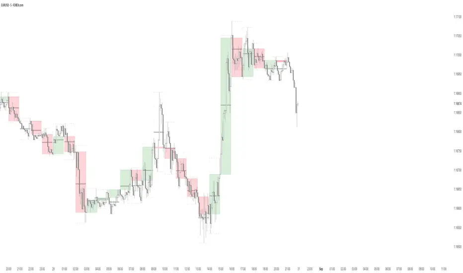
B A N K $ - HTF Candle Boxes (Power of 3)This indicator allows you to visualise the HTF candles on the LTF's, this is useful for using the Power of 3 / Accumulation, Manipulation & Distribution concepts.
By default, the HTF interval is set to 1h, this means that an outline will be created around the LTF candles that are within that 1h window. (i.e from 13:00-14:00 etc).
Features
HTF Interval Selector - this allows the user to customise which HTF interval to use
Candle Boxes - this outlines the full outer perimeter of the relevant candles
Include Body - this highlights the distance between the candle Open & Close
Show MidLine
Additional Settings
Hide Side Lines - this will only draw the Top & Bottom lines
Extend Lines to Current Candle - most recent Top & Bottom lines will extend to current price
Draw Lines from Exact Candle - this makes the most recent candle lines cleaner
I personally use this indicator to outline the most recent 3 1h candles to make it easier to identify sweeps & reversals however there is additional functionality to allow the user to customise the indicator to their preference.
Quantum Edge Scalper - Adaptive Precision Trading [KedArc Quant]Strategy Overview
Quantum Edge Scalper is a multi-regime intraday strategy engineered for adaptability across equities. It fuses EMA trend & slope, RSI sanity checks, ATR-based volatility gating, and candle-shape filters. Regime detection (ATR%% z-score) tunes thresholds on-the-fly, while an optional OSS — Oversold Short Override captures late-session breakdowns. Robust day-level controls include trade caps, cooldowns, and loss-streak stops. A compact panel summarizes live session stats.
Key Features
• Preset modes: Aggressive / Aggressive+ / Conservative / Hybrid / Custom.
• EMA Fast/Slow trend filter + EMA-separation slope gate.
• ATR volatility floor (percent-of-price) to avoid dead markets.
• Candle-shape and wick-ratio filters to curb false breakouts.
• Regime adaptation using ATR% z-score (HIGH / LOW / NEUTRAL).
• Hybrid+ LOW-regime extras: tighter SL, adaptive TP, mid-session pause, loss-streak blocker.
• OSS (Oversold Short Override): validators for micro-pullback, range expansion, structure break, and time window.
• Daily caps & loss-streak protection; cooldown management post wins/losses.
• Clean summary labels + compare panel; optional debug labels.

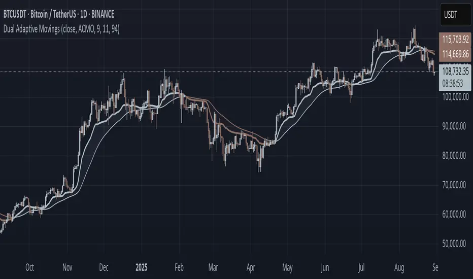
Dual Adaptive Movings### Dual Adaptive Movings
By Gurjit Singh
A dual-layer adaptive moving average system that adjusts its responsiveness dynamically using market-derived factors (CMO, RSI, Fractal Roughness, or Stochastic Acceleration). It plots:
* Primary Adaptive MA (MA): Fast, reacts to changes in volatility/momentum.
* Following Adaptive MA (FAMA): A smoother, half-alpha version for trend confirmation.
Instead of fixed smoothing, it adapts dynamically using one of four methods:
* ACMO: Adaptive CMO (momentum)
* ARSI: Adaptive RSI (relative strength)
* FRMA: Fractal Roughness (volatility + fractal dimension)
* ASTA: Adaptive Stochastic Acceleration (%K acceleration)
### ⚙️ Inputs & Options
* Source: Price input (default: close).
* Moving (Type): ACMO, ARSI, FRMA, ASTA.
* MA Length (Primary): Core adaptive window.
* Following (FAMA) Length: Optional; can match MA length.
* Use Wilder’s: Toggles Wilder vs EMA-style smoothing.
* Colors & Fill: Bullish/Bearish tones with transparency control.
### 🔑 How to Use
1. Identify Trend:
* When MA > FAMA → Bullish (fills bullish color).
* When MA < FAMA → Bearish (fills bearish color).
2. Crossovers:
* MA crosses above FAMA → Bullish signal 🐂
* MA crosses below FAMA → Bearish signal 🐻
3. Adaptive Edge:
* Select method (ACMO/ARSI/FRMA/ASTA) depending on whether you want sensitivity to momentum, strength, volatility, or acceleration.
4. Alerts:
* Built-in alerts trigger on crossovers.
### 💡 Tips
* Wilder’s smoothing is gentler than EMA, reducing whipsaws in sideways conditions.
* ACMO and ARSI are best for momentum-driven directional markets, but may false-signal in ranges.
* FRMA and ASTA excels in choppy markets where volatility clusters.
👉 In short: Dual Adaptive Movings adapts moving averages to the market’s own behavior, smoothing noise yet staying responsive. Crossovers mark possible trend shifts, while color fills highlight bias.
Trend by ΔMA + Double ZigZag + EMA/WMA Bands by KidevThis script is a multi-tool trend and structure analyzer combining moving average slope confirmation, double zigzag swing mapping, and dynamic EMA/WMA trend bands — all in one overlay indicator.
🔹 Key Features:
ΔMA Trend Detection
Detects trend shifts using the slope of a chosen moving average (SMA, EMA, WMA, RMA, HMA).
Confirms uptrend/downtrend only after a user-defined confirmation window.
Draws color-coded MA line (green = uptrend, red = downtrend, gray = sideways).
Optional arrows for trend change entries.
Alerts for confirmed trend shifts.
Double ZigZag Swing Analysis
Two customizable ZigZag layers with independent lookback periods.
Optional swing labels (HH, HL, LH, LL) to track market structure.
Full control over line style, width, and colors for each ZigZag.
EMA Band (96 default)
Plots a dynamic EMA channel (High, HLC3, Low).
Visual band highlights volatility and trend zones.
Adjustable fill color and transparency.
Weighted Moving Average (WMA 96)
Clean trend-following baseline.
Adjustable source, length, and color.
Background Highlight
Toggleable background shading for bullish / bearish / sideways conditions.
Fully customizable colors and transparency.
Helps visually separate market phases at a glance.
Note:
ZigZag repainting is inherent by design (future swings refine past points). Use it as a structural guide, not as a standalone signal.

ORB Breakouts with alerts"ORB Breakouts with Alerts" is a utility indicator that highlights an Opening Range Breakout (ORB) setup during a user-defined intraday time window. It allows traders to visualize price consolidation ranges and receive alerts when price breaks above or below the session high/low.
🔧 Features:
*Customizable session time (start and end), adjustable to local time using a timezone offset.
*Automatically plots:
*A shaded box around the session's high and low.
*Horizontal lines at session high and low levels.
*Optional "BUY"/"SELL" labels to mark breakout directions.
*Visual breakout signals when price crosses above or below the session range.
*Built-in alerts to notify when breakouts occur.
*Configurable styling options including box color, highlight color, and label placement.
⚙️ How It Works:
*During the defined time range, the script tracks the highest high and lowest low.
*After the session ends:
*A box is drawn to represent the opening range.
*Breakouts above the high or below the low trigger visual markers and optional alerts.
*Alerts are limited to one per direction per day to reduce noise.
⚠️ This indicator is a technical analysis tool only and does not provide financial advice or trade recommendations. Always use with proper risk management and in conjunction with your trading plan.

Multi HTF High/Low LevelsThis indicator plots the previous high and low from up to four user-defined higher timeframes (HTF), providing crucial levels of support and resistance. It's designed to be both powerful and clean, giving you a clear view of the market structure from multiple perspectives without cluttering your chart.
Key Features:
Four Customizable Timeframes: Configure up to four distinct higher timeframes (e.g., 1-hour, 4-hour, Daily, Weekly) to see the levels that matter most to your trading style.
Automatic Visibility: The indicator is smart. It automatically hides levels from any timeframe that is lower than your current chart's timeframe. For example, if you're viewing a Daily chart, the 4-hour levels won't be shown.
Clean On-Chart Lines: The high and low for each timeframe are displayed as clean, extended horizontal lines, but only for the duration of the current higher-timeframe period. This keeps your historical chart clean while still showing the most relevant current levels.
Persistent Price Scale Labels: For easy reference, the price of each high and low is always visible on the price scale and in the data window. This is achieved with an invisible plot, giving you the accessibility of a plot without the visual noise.
How to Use:
Go into the indicator settings.
Under each "Timeframe" group, check the "Show" box to enable that specific timeframe.
Select your desired timeframe from the dropdown menu.
The indicator will automatically calculate and display the previous high and low for each enabled timeframe.
Trade Calculator {Phanchai}Trade Calculator 🧮 {Phanchai} — Documentation
A lightweight sizing helper for TradingView that turns your risk per trade into an estimated maximum nominal position size — using the most recent chart low as your stop reference. Built for speed and clarity right on the chart.
Key Features
Clean on-chart info table with configurable font size and position.
Row toggles: show/hide each line (Price, Last Low, Risk per Trade, Entry − Low, SL to Low %, Max. Nominal Value in USDT).
Configurable low reference: Last N bars or Running since load .
Low label placed exactly at the wick of the lowest bar (no horizontal line).
Custom padding: add extra rows above/below and blank columns left/right (with custom whitespace/text fillers) to fine-tune layout.
Integer display for Risk per Trade (USDT) and Max. Nominal Value (USDT); decimals configurable elsewhere.
Open source script — easy to read and extend.
How to Use
Add the indicator: open TradingView → Indicators → paste the source code → Add to chart.
Pick your low reference in settings:
Last N bars — uses the lowest low within your chosen lookback.
Running since load — tracks the lowest low since the script loaded.
Set your capital and risk:
Total Capital — your account size in USDT.
Max. invest Capital per Trade (%) — your risk per trade as a percent of Total Capital.
Tidy the table:
Use Table Position and Table Size to place it.
Add Extra rows/columns and set left/right fillers (spaces allowed) for padding.
Toggle individual rows (on/off) to show only what you need.
Read the numbers:
Act. Price in USDT — current close.
Last Low in USDT — stop reference price.
Risk per Trade — whole-USDT value of your risk budget for this trade.
Entry − Low — absolute risk per unit.
SL to Low (%) — percentage distance from price to low.
Max. Nominal Value in USDT — estimated max nominal position size given your risk budget and stop at the low.
Scope
This calculator is designed for long trades only (stop below price at the chart low).
Notes & Assumptions
Does not factor fees, funding, slippage, tick size, or broker/venue position limits.
“Running since load” updates as new lows appear; “Last N bars” uses only the selected lookback window.
If price equals the low (zero distance), sizing will be undefined (division by zero guarded as “—”).
Risk Warning
Trading involves substantial risk. Always double-check every value the calculator shows, confirm your stop distance, and verify position sizing with your broker/platform before entering any order. Never risk money you cannot afford to lose.
Open Source & Feedback
The source code is open. If you spot a bug or have an idea to improve the tool, feel free to share suggestions — I’m happy to iterate and make it better.

Custom ORBIT — GSK-VIZAG-AP-INDIA 📌 Description
Custom ORBIT — Opening Range Breakout Indicator Tool
Created by GSK-VIZAG-AP-INDIA
This indicator calculates and visualizes the Opening Range (OR) of the trading session, with customizable start/end times and flexible range duration. The Opening Range is defined by the highest and lowest prices during the selected initial market window.
🔹 Key Features:
User-defined Opening Range duration (default: 15 minutes from 9:15).
Adjustable session start and end times.
Plots Opening Range High (ORH) and Opening Range Low (ORL).
Extends OR levels across the session with multiple line style options (Dotted, Dashed, Solid, Smoothed).
Highlights breakouts (price crossing above/below OR) and reversals (price returning back inside).
Simple chart markers (triangles/labels) for quick visual recognition.
⚠️ Disclaimer:
This tool is intended for educational and analytical purposes only. It does not generate buy/sell signals or provide financial advice. Always use independent analysis and risk management.

Realized Volatility (StdDev of Returns, %)Realized Volatility (StdDev of Returns, %)
This indicator measures realized (historical) volatility by calculating the standard deviation of log returns over a user-defined lookback period. It helps traders and analysts observe how much the price has varied in the past, expressed as a percentage.
How it works:
Computes close-to-close logarithmic returns.
Calculates the standard deviation of these returns over the selected lookback window.
Provides three volatility measures:
Daily Volatility (%): Standard deviation over the chosen period.
Annualized Volatility (%): Scaled using the square root of the number of trading days per year (default = 250).
Horizon Volatility (%): Scaled to a custom horizon (default = 5 days, useful for short-term views).
Inputs:
Lookback Period: Number of bars used for volatility calculation.
Trading Days per Year: Used for annualizing volatility.
Horizon (days): Adjusts volatility to a shorter or longer time frame.
Notes:
This is a statistical measure of past volatility, not a forecasting tool.
If you change the scale to logarithmic, the indicator readibility improves.
It should be used for analysis in combination with other tools and not as a standalone signal.