ABC on Recursive Zigzag [Trendoscope]There are several implementations of ABC pattern in tradingview and pine script. However, we have made this indicator to provide users additional quantifiable information along with flexibility to experiment and develop their own strategy based on the patterns.
🎲 Highlights of this indicator over other ABC implementations are:
Implementation is based on recursive multi level zigzag allows bigger as well as smaller patterns to be identified
Allows users to set their trading rules with respect to entry, target and stop ratios, experiment and build their own strategy based on the ABC pattern.
Back test summary including win ratio and risk reward will help users understand the profitability based on different settings being used.
🎲 Concept of ABC Pattern
The ABC pattern, also known as the "Corrective Wave" or "Zigzag Pattern," is a fundamental concept in Elliott Wave Theory, which is widely used in technical analysis to identify and predict price movements in financial markets.
The ABC pattern is a three-wave corrective pattern that typically occurs within the context of a larger impulse or trending wave. It consists of two smaller waves in the opposite direction (A and C) separated by a corrective wave (B). These waves are labeled alphabetically and represent price movements.
Wave A (Impulse Wave): Wave A is the first leg of the ABC pattern and is characterized by a strong price move in the opposite direction of the prevailing trend. It is often driven by a fundamental or sentiment-driven event that temporarily disrupts the trend.
Wave B (Corrective Wave): Wave B is the corrective wave that follows Wave A. It represents a partial retracement of Wave A's price movement. Wave B can take various forms, such as a simple correction or a complex correction (e.g., a triangle or a flat correction). It typically doesn't retrace the entire length of Wave A.
Wave C (Impulse Wave): Wave C is the final leg of the ABC pattern and is characterized by a strong price move in the same direction as the prevailing trend. It often surpasses the starting point of Wave A and confirms the resumption of the larger trend.
🎲 Indicator Components
Upon loading the indicator on the chart, we can observe the following components on the chart.
Pattern Drawings is the graphical representation of present patterns. Please note that it is not necessary for patterns to be there on the chart all the time. Patterns will appear on the chart when price makes the patterns.
Trade Box is the box representing trade signals of the pattern. These trade levels are generated based on the user settings.
Summary Table is the back test summary containing details of historical pattern performance including Win Ratio and Risk Reward.
🎲 Indicator Settings
Details of each user settings are provided in the tooltips. Below is the snapshot of it.
🎲 Alerts
Basic level of alerts are built in the script using alert function to highlight the following conditions:
New ABC Pattern
Updates to existing Pattern
Both conditions will alert simple text messages. There is not much customization provided as part of this indicator. We will consider providing more options in future versions based on the interest and demand shown by users.
Cari skrip untuk "wave"

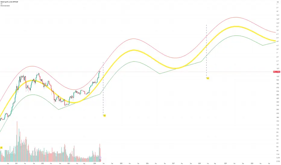
Bitcoin Market Cap wave model weeklyThis Bitcoin Market Cap wave model indicator is rooted in the foundation of my previously developed tool, the : Bitcoin wave model
To derive the Total Market Cap from the Bitcoin wave price model, I employed a straightforward estimation for the Total Market Supply (TMS). This estimation relies on the formula:
TMS <= (1 - 2^(-h)) for any h.This equation holds true for any value of h, which will be elaborated upon shortly. It is important to note that this inequality becomes the equality at the dates of halvings, diverging only slightly during other periods.
Bitcoin wave model is based on the logarithmic regression model and the sinusoidal waves, induced by the halving events.
This chart presents the outcome of an in-depth analysis of the complete set of Bitcoin price data available from October 2009 to August 2023.
The central concept is that the logarithm of the Bitcoin price closely adheres to the logarithmic regression model. If we plot the logarithm of the price against the logarithm of time, it forms a nearly straight line.
The parameters of this model are provided in the script as follows: log(BTCUSD) = 1.48 + 5.44log(h).
The secondary concept involves employing the inherent time unit of Bitcoin instead of days:
'h' denotes a slightly adjusted time measurement intrinsic to the Bitcoin blockchain. It can be approximated as (days since the genesis block) * 0.0007. Precisely, 'h' is defined as follows: h = 0 at the genesis block, h = 1 at the first halving block, and so forth. In general, h = block height / 210,000.
Adjustments are made to account for variations in block creation time.
The third concept revolves around investigating halving waves triggered by supply shock events resulting from the halvings. These halvings occur at regular intervals in Bitcoin's native time 'h'. All halvings transpire when 'h' is an integer. These events induce waves with intervals denoted as h = 1.
Consequently, we can model these waves using a sin(2pih - a) function. The parameter determining the time shift is assessed as 'a = 0.4', aligning with earlier expectations for halving events and their subsequent outcomes.
The fourth concept introduces the notion that the waves gradually diminish in amplitude over the progression of "time h," diminishing at a rate of 0.7^h.
Lastly, we can create bands around the modeled sinusoidal waves. The upper band is derived by multiplying the sine wave by a factor of 3.1*(1-0.16)^h, while the lower band is obtained by dividing the sine wave by the same factor, 3.1*(1-0.16)^h.
The current bandwidth is 2.5x. That means that the upper band is 2.5 times the lower band. These bands are forming an exceptionally narrow predictive channel for Bitcoin. Consequently, a highly accurate estimation of the peak of the next cycle can be derived.
The prediction indicates that the zenith past the fourth halving, expected around the summer of 2025, could result in Total Bitcoin Market Cap ranging between 4B and 5B USD.
The projections to the future works well only for weekly timeframe.
Enjoy the mathematical insights!
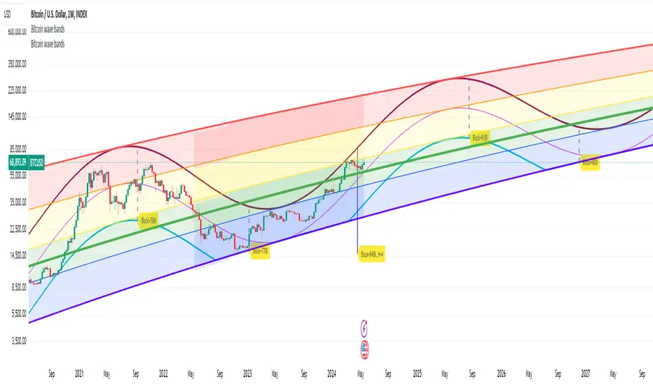
Bitcoin wave modelBitcoin wave model is based on the logarithmic regression model and the sinusoidal waves, induced by the halving events.
This chart presents the outcome of an in-depth analysis of the complete set of Bitcoin price data available from October 2009 to August 2023.
The central concept is that the logarithm of the Bitcoin price closely adheres to the logarithmic regression model. If we plot the logarithm of the price against the logarithm of time, it forms a nearly straight line.
The parameters of this model are provided in the script as follows: log (BTCUSD) = 1.48 + 5.44log(h).
The secondary concept involves employing the inherent time unit of Bitcoin instead of days:
'h' denotes a slightly adjusted time measurement intrinsic to the Bitcoin blockchain. It can be approximated as (days since the genesis block) * 0.0007. Precisely, 'h' is defined as follows: h = 0 at the genesis block, h = 1 at the first halving block, and so forth. In general, h = block height / 210,000.
Adjustments are made to account for variations in block creation time.
The third concept revolves around investigating halving waves triggered by supply shock events resulting from the halvings. These halvings occur at regular intervals in Bitcoin's native time 'h'. All halvings transpire when 'h' is an integer. These events induce waves with intervals denoted as h = 1.
Consequently, we can model these waves using a sin(2pih - a) function. The parameter determining the time shift is assessed as 'a = 0.4', aligning with earlier expectations for halving events and their subsequent outcomes.
The fourth concept introduces the notion that the waves gradually diminish in amplitude over the progression of "time h," diminishing at a rate of 0.7^h.
Lastly, we can create bands around the modeled sinusoidal waves. The upper band is derived by multiplying the sine wave by a factor of 3.1*(1-0.16)^h, while the lower band is obtained by dividing the sine wave by the same factor, 3.1*(1-0.16)^h.
The current bandwidth is 2.5x. That means that the upper band is 2.5 times the lower band. These bands are forming an exceptionally narrow predictive channel for Bitcoin. Consequently, a highly accurate estimation of the peak of the next cycle can be derived.
The prediction indicates that the zenith past the fourth halving, expected around the summer of 2025, could result in prices ranging between 200,000 and 240,000 USD.
Enjoy the mathematical insights!
Spread DifferentialThe Spread Differential tries to measure the speed of the market in any given direction. The histogram plots levels above or below zero in a sequence of Humps and Waves. Humps are repetitions of the previous trend before dropping to or near 0 whilst Waves are similar to Humps but the histogram must drop to or near 0 prior to forming another wave. You might notice that in no trend does the indicator ever form more than 2 waves. The indicator should be used in conjunction with the MA's selected in the panel to identify possible points of failure.

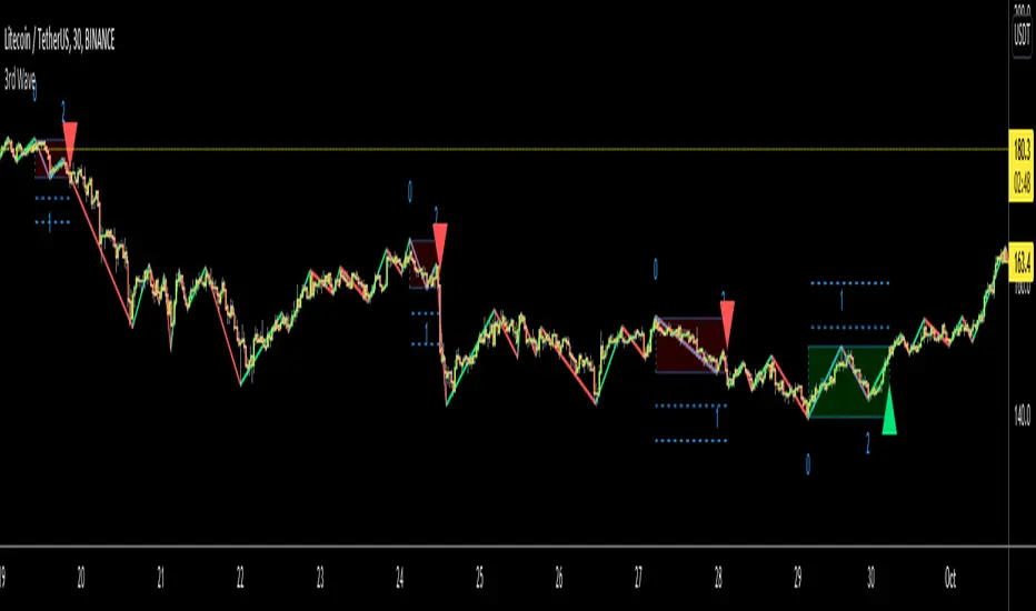
3rd WaveHello All,
In Elliott Wave Theory, 3rd wave is not the shortest one in the waves 1/3/5 and it's usually longest one. so if we can catch it then we may get good opportunities to trade. This script finds 3rd wave experimentally. it can be also the 3rd waves in the waves 1, 3, 5, A and C. the 3rd wave should have greater volume than other waves, the script can check its volume and compare with the volumes of the waves 1 and 2 optionally.
Pine Team released Pine version 5! This script was developed in v5 and it uses Library feature of Pine v5 for the zigzag functions. This script is also an example for the Pine developers who learn Pine v5 and Libraries.
Options:
Zigzag Period: is the length that is used to calculate highest/lowest and the zigzag waves
Min/Max Retracements: is the retracement rates to check the wave 2 according to wave 1. for example; if min/max values are 0.500-0.618 then wave 2 must be minimum 0.500 of wave 1 and maximum 0.618 of wave 1.
Check Volume Support: is an option to compare the volumes of1. 2. and . waves. if you enable this option then the script checks their volume and 3rd wave volume must be greater then 1 and 2
there are 4 options for the targets. you can enable/disable and change their levels. targets are calculated using length of wave 1.
Options to show breakout zone, zigzag, wave 1 and 2.
and some options for the colors.
The Library that is used in this script:
P.S. This is an experimental work and can be improved. So do not hesitate to drop your comments under the script ;)
Enjoy!
Smart WaveTrend Crossover█ OVERVIEW
Smart WaveTrend Crossover is an indicator based on WaveTrend crossovers, designed to reduce the number of false signals typically produced by classic oscillator crossovers.
Instead of triggering a signal immediately at the line crossover, the indicator requires additional confirmation in the form of a price breakout from a box, created at the moment of the WaveTrend signal.
The script also includes:
- a trend filter based on a separate WaveTrend
- “fog” visualization
- candle coloring based on trend direction
- fully configurable entry signals
- automatic Take Profit / Stop Loss levels
- a real-time TP/SL table
█ CONCEPTS
Classic WaveTrend crossovers often generate noise, especially during consolidation.
Smart WaveTrend Crossover attempts to address this issue using a breakout confirmation mechanism:
- at the moment WT1 crosses WT2, a horizontal price box is created
- a trade signal is generated only when price closes outside the box
- an optional trend filter limits signals to the dominant market direction
The trend filter is built on a WaveTrend crossover using larger, slower parameters, independent from the signal-generating WaveTrend.
This allows short-term momentum to be separated from the broader market direction, and all trend filter parameters can be freely adjusted.
WaveTrend signal settings are not identical to the original / classic values.
They are configured to generate a higher number of signals, which works better in combination with breakout boxes and confirmation logic.
Signal sensitivity can be easily adjusted by modifying channel length and averaging parameters.
By default, show_only_matching is enabled:
- bullish crossover → bullish breakout only (BUY)
- bearish crossover → bearish breakout only (SELL)
█ FEATURES
WaveTrend (Signals & Trend):
- two independent WaveTrend setups:
- one for signal generation
- one for trend determination
- signal parameters configured more aggressively than classic defaults
- trend filter based on a slower WaveTrend crossover
- trend direction visualized using directional fog, not a histogram
WaveTrend Input Explanation:
- Channel Length – controls WaveTrend reaction speed (shorter = more signals)
- Average Length – smoothing of the main WT1 line
- MA Length – smoothing of the signal line WT2
- Source – price source used in calculations (default: hlc3)
Fog (Visualization):
- visual representation of market pressure in the direction of the trend
- fog height based on average candle size × offset_mult
- adjustable transparency or fully disableable
Breakout Boxes:
- a box is created on every WaveTrend direction change
- default height based on the signal candle range
- optional box expansion using average candle size × box_multiplier
Signals:
- triangles or “BUY / SELL” labels
- direction matching filter (show_only_matching)
- option to display all breakouts regardless of crossover direction
- built-in BUY and SELL alerts
Visual Settings:
- candle coloring based on WaveTrend trend direction
- full control over bullish and bearish colors
Risk Management – TP / SL:
- automatic TP1, TP2, TP3 and SL levels
- two calculation modes:
- Candle Multiplier – based on average candle range
- Percentage – percentage from entry price
- separate parameters for each level
- TP/SL lines drawn on the chart
- real-time TP/SL price table
█ HOW TO USE
Add the indicator to your TradingView chart → Indicators → search “Smart WaveTrend Crossover”
Key settings:
- WaveTrend Settings for Signals – signal sensitivity
- WaveTrend Settings for Trend – market direction filter
- Signal Settings – signal type and box logic
- Fog – pressure visualization
- Risk Management – TP/SL configuration
Signal meaning:
- BUY → upward breakout from a box after a bullish crossover
- SELL → downward breakout from a box after a bearish crossover
- visible boxes → breakout watch zones
- fog and candle color → current market direction
█ APPLICATIONS
Standalone entry system
- entering directly on BUY / SELL signals
- or entering on trend color change
Filter for price-action strategies
- using WaveTrend signals as directional confirmation
- e.g. level breakout + WaveTrend confirmation = entry
Trend indicator
- trading other tools only in the direction of the WaveTrend trend
- e.g. RSI breaks above 50 while WaveTrend trend is bullish
█ NOTES
- Default settings are a starting point and may require adjustment
- The indicator works best as part of a broader trading system

Enhanced Neowave Wave 1 Finder with ZigZagThis script is an advanced technical analysis indicator for the TradingView platform, written in Pine Script version 5. Its primary goal is to identify potential Elliott Wave "Wave 1" patterns, enhanced with principles from Neowave theory and a custom ZigZag indicator for more accurate pivot detection. The script is designed to be overlaid on the main price chart.
Core Functionality: Blending ZigZag and Neowave
The indicator's methodology is a two-part process. First, it identifies significant price swings using a robust ZigZag indicator. Then, it analyzes these swings based on a set of rules derived from Neowave and classic technical analysis to validate them as potential Wave 1 patterns.
Part 1: ZigZag Integration
The first major component is a comprehensive ZigZag indicator that forms the foundation for all subsequent analysis.
Pivot Detection: The pivots() function is the engine of the ZigZag. It scans the historical price data for significant high and low points (pivots) over a user-defined Length.
Segment Drawing: Once pivots are identified, the script draws lines connecting them, creating the classic ZigZag pattern on the chart.
Extended Direction & Ratios: This is an enhanced feature. The script doesn't just identify highs and lows; it categorizes them as:
Higher High (HH) or Lower High (LH)
Lower Low (LL) or Higher Low (HL)
This classification is crucial for understanding the market structure. It also calculates the price ratio of the most recent ZigZag leg relative to the previous one, which is used later for pattern validation.
Dynamic Updates: The ZigZag is not static. On each new bar, it can update its most recent pivot point if a new, more extreme price (a higher high or a lower low) is printed before the direction officially changes. This ensures the ZigZag is always reflecting the most current and significant price action.
Part 2: Neowave Wave 1 Finder
With the market structure defined by the ZigZag, the second part of the script applies a rigorous set of rules to identify potential Wave 1 patterns. A Wave 1 is the initial move of a new trend in Elliott Wave theory.
Key Validation Criteria
For a price move between two ZigZag pivots to be considered a valid Wave 1, it must pass a series of checks:
Significance: The move must have a minimum percentage change (Minimum Wave Length) and last for a minimum number of bars, filtering out insignificant noise.
Volume Confirmation: A genuine impulse wave is typically supported by increasing volume. The script checks if the volume during the potential Wave 1 is significantly higher than the recent average (Volume Increase Threshold).
Momentum Alignment: The direction of the wave must be confirmed by momentum indicators.
For a bullish (upward) Wave 1, the Relative Strength Index (RSI) must be in a bullish regime (above 50) and the MACD line must be above its signal line.
For a bearish (downward) Wave 1, the RSI must be below 50 and the MACD line must be below its signal line.
Structural Analysis (Impulse vs. Diagonal): The script attempts to differentiate between two types of Wave 1:
Impulse Wave: A strong, clean, and direct move.
Diagonal Wave: A more complex, overlapping, and often wedge-shaped pattern. This is identified by analyzing the time and price complexity of the move, along with the ZigZag leg ratios.
Wave 2 Retracement Check: A critical Neowave rule is that a valid Wave 1 must be followed by a valid Wave 2 retracement. The script looks at the next ZigZag leg to ensure it doesn't retrace more than 100% of the potential Wave 1. It also uses the ZigZag ratios to confirm the retracement falls within typical Fibonacci levels (e.g., 38.2% to 78.6%).
Display and User Interface
The script provides a rich visual experience to aid the trader in their analysis.
Wave Labels and Boxes: When a valid Wave 1 is detected, it is highlighted with a colored line (green for bullish, red for bearish) and a shaded background box. A label clearly marks it as "Wave 1 IMPULSE" or "Wave 1 DIAGONAL".
Fibonacci Retracement Levels: Upon detection of a Wave 1, the script automatically draws key Fibonacci retracement levels (38.2%, 50%, 61.8%, 78.6%). These levels are potential targets for the end of the subsequent Wave 2, offering potential entry points for a Wave 3 trade.
Information Labels: Additional labels provide at-a-glance confirmation of the conditions, showing whether volume and momentum criteria were met.
Customizable Inputs: Users have extensive control over the indicator's parameters, including the ZigZag length, volume thresholds, RSI levels, and the colors of all visual elements.
Alerts: The indicator can be configured to generate an alert whenever a new bullish or bearish Wave 1 pattern is confirmed, allowing traders to be notified of potential opportunities in real-time.

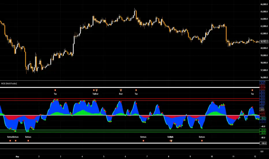
Market Cipher B by WeloTradesMarket Cipher B by WeloTrades: Detailed Script Description
//Overview//
"Market Cipher B by WeloTrades" is an advanced trading tool that combines multiple technical indicators to provide a comprehensive market analysis framework. By integrating WaveTrend, RSI, and MoneyFlow indicators, this script helps traders to better identify market trends, potential reversals, and trading opportunities. The script is designed to offer a holistic view of the market by combining the strengths of these individual indicators.
//Key Features and Originality//
WaveTrend Analysis:
WaveTrend Channel (WT1 and WT2): The core of this script is the WaveTrend indicator, which uses the smoothed average of typical price to identify overbought and oversold conditions. WT1 and WT2 are calculated to track market momentum and cyclical price movements.
Major Divergences (🐮/🐻): The script detects and highlights major bullish and bearish divergences automatically, providing traders with visual cues for potential reversals. This helps in making informed decisions based on divergence patterns.
Relative Strength Index (RSI):
RSI Levels: RSI is used to measure the speed and change of price movements, with specific levels indicating overbought and oversold conditions.
Customizable Levels: Users can configure the overbought and oversold thresholds, allowing for a tailored analysis based on individual trading strategies.
MoneyFlow Indicator:
Fast and Slow MoneyFlow: This indicator tracks the flow of capital into and out of the market, offering insights into the underlying market strength. It includes configurable periods and multipliers for both fast and slow MoneyFlow.
Vertical Positioning: The script allows users to adjust the vertical position of MoneyFlow plots to maintain a clear and uncluttered chart.
Stochastic RSI:
Stochastic RSI Levels: This combines the RSI and Stochastic indicators to provide a momentum oscillator that is sensitive to price changes. It is used to identify overbought and oversold conditions within a specified period.
Customizable Levels: Traders can set specific levels for more precise analysis.
//How It Works//
The script integrates these indicators through advanced algorithms, creating a synergistic effect that enhances market analysis. Here’s a detailed explanation of the underlying concepts and calculations:
WaveTrend Indicator:
Calculation: WaveTrend is based on the typical price (average of high, low, and close) smoothed over a specified channel length. WT1 and WT2 are derived from this typical price and further smoothed using the Average Channel Length. The difference between WT1 and WT2 indicates momentum, helping to identify cyclical market trends.
RSI (Relative Strength Index):
Calculation: RSI calculates the average gains and losses over a specified period to measure the speed and change of price movements. It oscillates between 0 and 100, with levels set to identify overbought (>70) and oversold (<30) conditions.
MoneyFlow Indicator:
Calculation: MoneyFlow is derived by multiplying price changes by volume and smoothing the results over specified periods. Fast MoneyFlow reacts quickly to price changes, while Slow MoneyFlow offers a broader view of capital movement trends.
Stochastic RSI:
Calculation: Stochastic RSI is computed by applying the Stochastic formula to RSI values, which highlights the RSI’s relative position within its range over a given period. This helps in identifying momentum shifts more precisely.
//How to Use the Script//
Display Settings:
Users can enable or disable various components like WaveTrend OB & OS levels, MoneyFlow plots, and divergence alerts through checkboxes.
Example: Turn on "Show Major Divergence" to see major bullish and bearish divergence signals directly on the chart.
Adjust Channel Settings:
Customize the data source, channel length, and smoothing periods in the "WaveTrend Channel SETTINGS" group.
Example: Set the "Channel Length" to 10 for a more responsive WaveTrend line or adjust the "Average Channel Length" to 21 for smoother trends.
Set Overbought & Oversold Levels:
Configure levels for WaveTrend, RSI, and Stochastic RSI in their respective settings groups.
Example: Set the WaveTrend Overbought Level to 60 and Oversold Level to -60 to define critical thresholds.
Money Flow Settings:
Adjust the periods and multipliers for Fast and Slow MoneyFlow indicators, and set their vertical positions for better visualization.
Example: Set the Fast Money Flow Period to 9 and Slow Money Flow Period to 12 to capture both short-term and long-term capital movements.
//Justification for Combining Indicators//
Enhanced Market Analysis:
Combining WaveTrend, RSI, and MoneyFlow provides a more comprehensive view of market conditions. Each indicator brings a unique perspective, making the analysis more robust.
WaveTrend identifies cyclical trends, RSI measures momentum, and MoneyFlow tracks capital movement. Together, they provide a multi-dimensional analysis of the market.
Improved Decision-Making:
By integrating these indicators, the script helps traders make more informed decisions. For example, a bullish divergence detected by WaveTrend might be validated by an RSI moving out of oversold territory and supported by increasing MoneyFlow.
Customization and Flexibility:
The script offers extensive customization options, allowing traders to tailor it to their specific needs and strategies. This flexibility makes it suitable for different trading styles and timeframes.
//Conclusion//
The indicator stands out due to its innovative combination of WaveTrend, RSI, and MoneyFlow indicators, offering a well-rounded tool for market analysis. By understanding how each component works and how they complement each other, traders can leverage this script to enhance their market analysis and trading strategies, making more informed and confident decisions.
Remember to always backtest the indicator first before implying it to your strategy.
NET BSP NET BSP derived from Buying & Selling Pressure which is a volatility indicator that monitors average metrics of green and red candles separately.
We could navigate more confidently through market with projected market balance.
BSP allowed us to track and analyze the ongoing performance of bullish and bearish impulsive waves and their corrections.
Due to unintuitive way of measuring decline with SP going up, I decided to remake it into more intuitive version with better precision.
When we encounter the fall it's better to have declining values of tool to be able to cover it visually with ease.
One of the solutions was to create a sense of balance of Buying Pressure against Selling Pressure.
Since we are oriented by growth, it'd be more logical to summarize the market balance with BP - SP
Comparison:
When Buying and Selling Pressure are equal, NET BSP would be at 0.
NETBSP > 0 and NETBSP > NETBSP = 🟢
NETBSP > 0 and NETBSP < NETBSP = 🟡
NETBSP < 0 and NETBSP < NETBSP = 🔴
NETBSP < 0 and NETBSP > NETBSP = 🟡
Hence, we get visualized stages of uptrends and downtrends which allows to evaluate chances and estimations of upcoming counter-waves.
Also, it is worth to note that output clearly shows how one wave is derived from another in terms of sizing.
Feel free to adjust NET BSP arguments to adapt sensitivity to the timeframe you're working on.

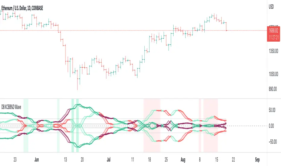
DB KCBB%D WavesDB KCBB%D Waves
What does the indicator do?
The indicator plots the percent difference between the low and high prices against a combined Kelpler Channel Bollinger Bands for the current timeframe. The low percent difference and the high percent difference each have their own waves plotted. A mirror mode default allows both waves to be visualized in a mirrored plot that clearly shows when outer bands are present and when they swap. Each percent difference band is displayed with a 1 bar lookback to visualize local tops/bottoms.
The overall trend is displayed using two sets of green/red colors on the percent difference waves so that each wave is recognizable, but the overall price trend is visible. A fast 3 SMA is taken of each percent difference wave to obtain the overall trend and then averaged together. The trend is then calculated based on direction from the previous bar period.
How should this indicator be used?
By default, the indicator will display in a mirror mode which will display both the low and high percent change waves mirrored to allow for the most pattern recognition possible. You will notice the percent difference waves swap from inner to outer, showing the overall market direction for that timeframe. When each percent difference wave interacts with the zero line, it indicates either buys or sells opportunities depending on which band is on the inside. When the inner wave crosses zero, special attention should be paid to the outer wave to know if it's a significant move. Likewise, when the outer wave peaks, it can indicate buy or sell opportunities depending on which wave is on the outside.
A zero line and other lines are displayed from the highest of the high percent difference wave over a long period of time. The lines can measure movement and possible oversold/overbought locations or large volatility. You can also use the lines for crossing points for either wave as alerts to know when to buy or sell zones are happening.
When individual percent difference waves are designed to be reviewed without mirroring, the mirror checkbox can be unchecked in the settings. Doing so will display both the high and low percent difference waves separately. Using this display, you can more cleanly review how each wave interacts with various line levels.
For those who desire to only have half of the mirror or one set of waves inverted against each other, check the "mirrored" and the "mirrored flipped" checkboxes in the settings. Doing so will display the top half of the mirror indicator, which is the low percent difference wave with the high percent difference wave inverted.
The indicator will also change the background color of its own pane to indicate possible buy/sell periods (work in progress).
Does the indicator include any alerts?
Yes, they are a work in progress but starting out with this release, we have:
NOTE: This is an initial release version of this indicator. Please do not use these alerts with bots yet, as they will repaint in real-time.
NOTE: A later release may happen that will delay firing the events until 1/2 of the current bar time has passed.
NOTE: As with any indicator watch your upper timeframe waves first before zooming into lower.
DB KCBB%D Buy Zone Alert
DB KCBB%D MEDIUM Buy Alert
DB KCBB%D STRONG Buy Alert
DB KCBB%D Sell Alert
DB KCBB%D STRONG Sell Alert
DB KCBB%D Trend Up Alert
DB KCBB%D Trend Down Alert
Use at your own risk and do your own diligence.
Enjoy!
OpenCipher AOpenCipher A is an open-source and free to use Overlay.
Features:
EMA Ribbons (Lengths: 5, 11, 15, 18, 21, 25, 29, 33)
Symbols ("Be careful" and "attention required" signals)
EMA Ribbons
The EMA RIbbons are a set of exponential moving averages. Blue and white ribbons = uptrend, gray ribbons = downtrend. The ribbons can act as support in uptrends and as resistance in downtrends.
Lengths and source of the ribbons are customizable.
Symbols
Green Dots: The green dot is a bullish symbol that appears whenever the EMA 11 crosses over EMA 33.
Red Cross: The red cross is a bearish symbol that appears whenever the EMA 5 crosses under EMA 11.
Blue Triangle: The blue triangle marks a possible trend reversal that appears whenever the EMA 5 crosses over EMA 25 while EMA 29 is below EMA 33.
Red Diamond: The red diamond is a bearish symbol that marks a potential local top whenever a bearish wavecross occurs (fast wave crosses under slow wave).
Yellow X: The yellow X is a warning signal that appears whenever a bearish wavecross occurs while the slow wave of the wavetrend is below -40 and the moneyflow is in the red (below zero).
Blood Diamond: The blood diamond is a bearish symbol that highlights whenever the red diamond and the red cross appear on the same candle.
Usage
Treat the symbols as signs that your attention might be required and don't trade based on them.

Hull Volume WavesInspired by the works of David Weis, this indicator is an alternative to his classic Weis Volume Waves.
As the name implies, this indicator uses a Hull Moving Average to detect price swings, and calculates the cumulative volume for each of them, separating the up swings from the down swings.
The chosen length of the HMA determines the size of each swing, meaning lower lengths will detect microswings while higher lengths will only include the main swings.
The length of each swing also determines the color of the upward and downward waves, and you can choose 2 colors each to generate a bullish and bearish gradient.
Extreme values are highlighted in the background. The indicator will compare the current up wave to the last N up volumes, or the current down wave to the last N down volumes. The lookback length can be changed in the menu.
I hope you find it useful!

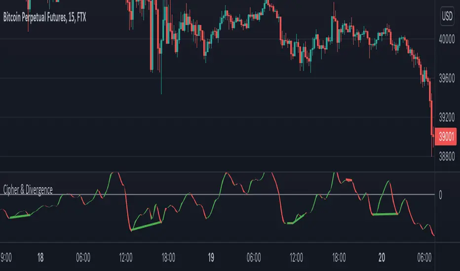
Cipher & DivergenceFor a long time I've been using complicated script with too much informations in it.
In this one I try to have just the bare minimum information to be able to analyse and find a potential reversal zone.
It is inspired from different wave trend / cipher script but has been tuned after months of backtest.
Extending the usage of the wave trend oscillator, which can be used with overbuy & oversell zone it might be better to wait for a confirmation of the movement. This confirmation can be identified by a pull back of the wave trend & price.
We can even confort ourself by waiting for reversal indicators.
Reversal may occurs after a divergence, wait for it, a cross of zero line followed by a PB to find your entry.
You can setup alert on bear / bull divergence but also when the wave trend cross the zero line to never miss a potential trade.
Huge thanks to LazyBear for his wave trend
And thanks vumanchu for his huge cipher script which was very useful for divergence finder
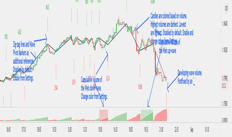
Weis Wave Volume NumbersWhat is it?
This is an indicator to complement @modhelius' Weis Wave Volume Indicator.
Original code has been modified to display wave volume (cumulative) numbers above or below the latest candle of the corresponding wave on the main pane. Since we are concerned only with relative volume, VOLUME NUMBERS HAVE BEEN SCALED DOWN. (If you need actual volume numbers, uncheck "Scale Down Volume" option in Settings). Rising wave volume is denoted in green. Falling wave volume is denoted in red. Developing wave volume is postfixed with a '_'. Confirmed wave volumes won't have this.
Who is it for?
This indicator is useful if you already use Weis Waves in your analysis and could do with an additional numerical representation of the wave volume on the main pane. Can be used in conjunciton with @modhelius' Weis Wave Volume (WWV) indicator (need to be added separately) to complement the visual representation of the waves. Can be used independently as well.
Pelase note that if you use any other Weis Wave indicator (other than @modhelius'), the numbers and the waveforms might not match.
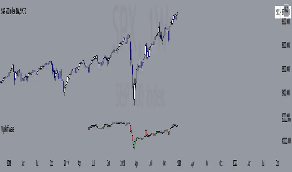
Wyckoff Wave"The Wyckoff Wave is a weighted index consisting of 12 stocks that are leaders in their perspective industries. It was introduced by the Stock Market Institute in 1931.
Made up of leaders in the important stock groups, the Wyckoff Wave represents the core of the American industrial complex.
The Wyckoff Wave has been a market indicator for Wyckoff students for over 50 years. While the stocks comprising the Wyckoff Wave have changed over time, it continues to be a sensitive leading market indicator. The Wyckoff Wave has consistently identified market trends.
The Wyckoff Wave is extremely helpful in predicting the stock market’s timing and the direction of the next market move.
The Wyckoff Wave is analyzed in five minute intervals and individual up and down iintra-day waves are created.
These individual waves, which include the price action and volume during those brief up and down market swings, also provide the data for other important Wyckoff Stock Market Institute indicators, including the Optimism-Pessimism volume index and the Trend Barometer.
These 12 stocks that make up the Wyckoff Wave. They are listed, along with their multipliers, below."
Wave Stock / Multiplier
AT&T / 79
Bank of America / 50
Boeing / 39
Bristol Myers / 119
Caterpillar / 35
DowDuPont / 72
Exxon Mobile / 32
IBM / 21
General Electric / 90
Ford / 25
Union Pacific / 60
WalMart / 43
In 2019, DowDuPont split into three companies: Dow, DuPont, and Corteva. Because TV limits the number of securities in a script to 40, only Dow and DuPont are factored into the Wave calculation (higher market caps than Corteva) with a multiplier of 36 each.
Renko Weis Wave VolumeThis is live and non-repainting Renko Weis Wave Volume tool. The tool has it’s own engine and not using integrated function of Trading View.
Renko charts ignore time and focus solely on price changes that meet a minimum requirement. Time is not a factor on Renko chart but as you can see with this script Renko RSI created on time chart.
Renko chart provide several advantages, some of them are filtering insignificant price movements and noise, focusing on important price movements and making support/resistance levels much easier to identify.
As source Closing price or High/Low can be used.
Traditional or ATR can be used for scaling. If ATR is chosen then there is rounding algorithm according to mintick value of the security. For example if mintick value is 0.001 and brick size (ATR/Percentage) is 0.00124 then box size becomes 0.001. And also while using dynamic brick size (ATR), box size changes only when Renko closing price changed.
This tool is based on the Weis Wave described by David H. Weis (a Wyckoff specialist). The Weis Waves Indicator sums up volumes in each wave. This is how we receive a bar chart of cumulative volumes of alternating waves and The cumulative volume makes the Weis wave charts unique.
If there is no volume information for the security then this tool has an option to use “True Range” instead of volume .
Better to use this script with the following one:
Enjoy!

Point and Figure (PnF) Weis Wave VolumeThis is live and non-repainting Point and Figure Chart Weis Wave Volume tool. The script has it’s own P&F engine and not using integrated function of Trading View.
Point and Figure method is over 150 years old. It consist of columns that represent filtered price movements. Time is not a factor on P&F chart but as you can see with this script P&F chart created on time chart.
P&F chart provide several advantages, some of them are filtering insignificant price movements and noise, focusing on important price movements and making support/resistance levels much easier to identify.
This tool is based on the Weis Wave described by David H. Weis (a Wyckoff specialist). The Weis Waves Indicator sums up volumes in each wave. This is how we receive a bar chart of cumulative volumes of alternating waves and The cumulative volume makes the Weis wave charts unique.
If there is no volume information for the security then this tool has an option to use “True Range” instead of volume .
If you are new to Point & Figure Chart then you better get some information about it before using this tool. There are very good web sites and books. Please PM me if you need help about resources.
Options in the Script
Box size is one of the most important part of Point and Figure Charting. Chart price movement sensitivity is determined by the Point and Figure scale. Large box sizes see little movement across a specific price region, small box sizes see greater price movement on P&F chart. There are four different box scaling with this tool: Traditional, Percentage, Dynamic (ATR), or User-Defined
4 different methods for Box size can be used in this tool.
User Defined: The box size is set by user. A larger box size will result in more filtered price movements and fewer reversals. A smaller box size will result in less filtered price movements and more reversals.
ATR: Box size is dynamically calculated by using ATR, default period is 20.
Percentage: uses box sizes that are a fixed percentage of the stock's price. If percentage is 1 and stock’s price is $100 then box size will be $1
Traditional: uses a predefined table of price ranges to determine what the box size should be.
Price Range Box Size
Under 0.25 0.0625
0.25 to 1.00 0.125
1.00 to 5.00 0.25
5.00 to 20.00 0.50
20.00 to 100 1.0
100 to 200 2.0
200 to 500 4.0
500 to 1000 5.0
1000 to 25000 50.0
25000 and up 500.0
Default value is “ATR”, you may use one of these scaling method that suits your trading strategy.
If ATR or Percentage is chosen then there is rounding algorithm according to mintick value of the security. For example if mintick value is 0.001 and box size (ATR/Percentage) is 0.00124 then box size becomes 0.001.
And also while using dynamic box size (ATR or Percentage), box size changes only when closing price changed.
Reversal : It is the number of boxes required to change from a column of Xs to a column of Os or from a column of Os to a column of Xs. Default value is 3 (most used). For example if you choose reversal = 2 then you get the chart similar to Renko chart.
Source: Closing price or High-Low prices can be chosen as data source for P&F charting.
There is only one option for Weis Wave Volume, “Use True Range (if no Volume info)” if you select this option and volume info is not avaliable then it uses “true range”, but if volume info is available, it never use true range. Default value is set to use true range.

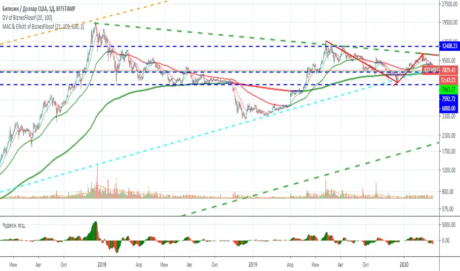
Moving Average Channel and Elliott of BiznesFilosofThis indicator is based on my indicator "MAC of BiznesFilosof", but it differs in that it shows three waves. Daily, weekly and monthly wave. Based on the color of these waves, you can easily determine the trend to use the indicator in combination with oscillators.
The main idea of this indicator is ease of use. Although I made it possible to show the corridor in the settings, but I consider it more convenient when there is a minimum of heaps on the chart. The color of the moving average perfectly shows when overbought and oversold. The idea is that the asset value is slower than the price. And it helps to enter the transaction correctly.
More details will be on my channel in YouTube.
===
Этот индикатор создан на базе моего индикатора "MAC of BiznesFilosof", но он отличается тем, что показывает три волны. Волна дневная, недельная и месячная. На основании цвета этих волн можно легко определить тренд, чтобы использовать индикатор в сочетании с осциляторами.
Основная идея данного индикатора - это простота использования. Хоть я и сделал возможность в настройках показать коридор, но считаю более удобным, когда на графике минимум нагромождений. Цвет скользящей средней прекрасно показывает, когда перекупленность и перепроданность. Идея состоит в том, что ценность актива более медленная, чем цена. И это помогает правильно входить в сделку.
Больше подробностей будет на моём канале в Ютуб.
Fractal Resonance BarLazyBear's WaveTrend port has been praised for highlighting trend reversals with precision and punctuality (minimal lag). But strong "3rd Wave" trends can "embed" or saturate any oscillator flashing several premature crosses while stuck overbought/oversold. This happens when the trend stretches over a longer timescale than the oscillator's averaging window or filter time constant. Our solution: monitor many timescales. With Fractal Resonance Bar's rich color codings, strong wavefronts form across timescales and jump out like an approaching line of thunderclouds!
Fractal Resonance Bar color-codes the status of eight underlying stochastic oscillators, with each row averaging over twice the time of the row above.
Fractal Resonance Bar shifts its timescales along with your choice of main chart timescale:
1 minute chart: 1 minute through 128 minute (~2 hour) oscillators.
15 minute chart: 15 minute through 1920 minute (~32 hour) oscillators.
1 hour chart: 1 hour through 128 hour (~2 week) oscillators.
Daily chart: 1 day through 128 day (~4 month) oscillators.
The color map is configured as follows:
Hot Pink: Extreme Overbought (> 100%) rolled over to sell, but oscillators probably embedded with more upside (revert to Dark Green) possible after a pause.
Deep Red: Overbought (> 75%) crossover ripe for selling (validated when red spreads to timescales below).
Brown: Minor (< 75%) crossover sell from which could bounce back green or start a plunge toward gray/black.
Gray/Black: Mature (< -75%) sells turning full black in a plunge before the dawn.
Lime Green: Extreme Oversold (< -100%) and bouncing, though may yet bottom even lower.
Green: Oversold (< -75%) crossover ripe for buy. Green spreading to all timescales below will validate bottom is in.
Dark Green/Teal: Mature buy in overbought (> 75%) range, waiting for sell crossover to Hot Pink for a pause or correction.
White Stripes are Impulsive Trend Warning
Fractal Resonance Bar warns of oscillator embedding by showing white stripes when it detects strong, early surges in the timescale rows below.The white stripes usually accompany Hot Pink warning it's too early to go short, or Lime Green warning it's too early to go long.
Heeding these warnings will probably miss the exact top or bottom, but you're less likely to get overrun in a momentum move.
Usually the market gives us a second opportunity to short very close to the top or buy very close to the bottom after the warning white stripes have subsided.
NOTE: Recently rolled over Futures contracts may not have enough history for all oscillator calculations, in which case no bar colors will appear.
Tweakable Attributes
The default Channel Length, Stochastic Ratio Length and Lag Length work reasonably well on all timescales in our experience. Minor tweaks don't hurt but this may just overfit to a particular chart history.
We don't recommend changing the 75% Overbought and 100% Extreme Overbought default levels as these are ideal numbers relative to the underlying oscillator statistic calculations. But these settings can shift the color transition levels.
Embedded attribute controls the sensitivity/conservativeness of the white strip embedding detectors. Closer to 75 increases the warning sensitivity while closer to 100 decreases the aggressiveness of blocking white stripes.
Embed Separation also affects the white stripe sensitivity.
Row width increases each row's thickness to fill the available screen height you've afforded the bar.

Adaptive Market Wave TheoryAdaptive Market Wave Theory
🌊 CORE INNOVATION: PROBABILISTIC PHASE DETECTION WITH MULTI-AGENT CONSENSUS
Adaptive Market Wave Theory (AMWT) represents a fundamental paradigm shift in how traders approach market phase identification. Rather than counting waves subjectively or drawing static breakout levels, AMWT treats the market as a hidden state machine —using Hidden Markov Models, multi-agent consensus systems, and reinforcement learning algorithms to quantify what traditional methods leave to interpretation.
The Wave Analysis Problem:
Traditional wave counting methodologies (Elliott Wave, harmonic patterns, ABC corrections) share fatal weaknesses that AMWT directly addresses:
1. Non-Falsifiability : Invalid wave counts can always be "recounted" or "adjusted." If your Wave 3 fails, it becomes "Wave 3 of a larger degree" or "actually Wave C." There's no objective failure condition.
2. Observer Bias : Two expert wave analysts examining the same chart routinely reach different conclusions. This isn't a feature—it's a fundamental methodology flaw.
3. No Confidence Measure : Traditional analysis says "This IS Wave 3." But with what probability? 51%? 95%? The binary nature prevents proper position sizing and risk management.
4. Static Rules : Fixed Fibonacci ratios and wave guidelines cannot adapt to changing market regimes. What worked in 2019 may fail in 2024.
5. No Accountability : Wave methodologies rarely track their own performance. There's no feedback loop to improve.
The AMWT Solution:
AMWT addresses each limitation through rigorous mathematical frameworks borrowed from speech recognition, machine learning, and reinforcement learning:
• Non-Falsifiability → Hard Invalidation : Wave hypotheses die permanently when price violates calculated invalidation levels. No recounting allowed.
• Observer Bias → Multi-Agent Consensus : Three independent analytical agents must agree. Single-methodology bias is eliminated.
• No Confidence → Probabilistic States : Every market state has a calculated probability from Hidden Markov Model inference. "72% probability of impulse state" replaces "This is Wave 3."
• Static Rules → Adaptive Learning : Thompson Sampling multi-armed bandits learn which agents perform best in current conditions. The system adapts in real-time.
• No Accountability → Performance Tracking : Comprehensive statistics track every signal's outcome. The system knows its own performance.
The Core Insight:
"Traditional wave analysis asks 'What count is this?' AMWT asks 'What is the probability we are in an impulsive state, with what confidence, confirmed by how many independent methodologies, and anchored to what liquidity event?'"
🔬 THEORETICAL FOUNDATION: HIDDEN MARKOV MODELS
Why Hidden Markov Models?
Markets exist in hidden states that we cannot directly observe—only their effects on price are visible. When the market is in an "impulse up" state, we see rising prices, expanding volume, and trending indicators. But we don't observe the state itself—we infer it from observables.
This is precisely the problem Hidden Markov Models (HMMs) solve. Originally developed for speech recognition (inferring words from sound waves), HMMs excel at estimating hidden states from noisy observations.
HMM Components:
1. Hidden States (S) : The unobservable market conditions
2. Observations (O) : What we can measure (price, volume, indicators)
3. Transition Matrix (A) : Probability of moving between states
4. Emission Matrix (B) : Probability of observations given each state
5. Initial Distribution (π) : Starting state probabilities
AMWT's Six Market States:
State 0: IMPULSE_UP
• Definition: Strong bullish momentum with high participation
• Observable Signatures: Rising prices, expanding volume, RSI >60, price above upper Bollinger Band, MACD histogram positive and rising
• Typical Duration: 5-20 bars depending on timeframe
• What It Means: Institutional buying pressure, trend acceleration phase
State 1: IMPULSE_DN
• Definition: Strong bearish momentum with high participation
• Observable Signatures: Falling prices, expanding volume, RSI <40, price below lower Bollinger Band, MACD histogram negative and falling
• Typical Duration: 5-20 bars (often shorter than bullish impulses—markets fall faster)
• What It Means: Institutional selling pressure, panic or distribution acceleration
State 2: CORRECTION
• Definition: Counter-trend consolidation with declining momentum
• Observable Signatures: Sideways or mild counter-trend movement, contracting volume, RSI returning toward 50, Bollinger Bands narrowing
• Typical Duration: 8-30 bars
• What It Means: Profit-taking, digestion of prior move, potential accumulation for next leg
State 3: ACCUMULATION
• Definition: Base-building near lows where informed participants absorb supply
• Observable Signatures: Price near recent lows but not making new lows, volume spikes on up bars, RSI showing positive divergence, tight range
• Typical Duration: 15-50 bars
• What It Means: Smart money buying from weak hands, preparing for markup phase
State 4: DISTRIBUTION
• Definition: Top-forming near highs where informed participants distribute holdings
• Observable Signatures: Price near recent highs but struggling to advance, volume spikes on down bars, RSI showing negative divergence, widening range
• Typical Duration: 15-50 bars
• What It Means: Smart money selling to late buyers, preparing for markdown phase
State 5: TRANSITION
• Definition: Regime change period with mixed signals and elevated uncertainty
• Observable Signatures: Conflicting indicators, whipsaw price action, no clear momentum, high volatility without direction
• Typical Duration: 5-15 bars
• What It Means: Market deciding next direction, dangerous for directional trades
The Transition Matrix:
The transition matrix A captures the probability of moving from one state to another. AMWT initializes with empirically-derived values then updates online:
From/To IMP_UP IMP_DN CORR ACCUM DIST TRANS
IMP_UP 0.70 0.02 0.20 0.02 0.04 0.02
IMP_DN 0.02 0.70 0.20 0.04 0.02 0.02
CORR 0.15 0.15 0.50 0.10 0.10 0.00
ACCUM 0.30 0.05 0.15 0.40 0.05 0.05
DIST 0.05 0.30 0.15 0.05 0.40 0.05
TRANS 0.20 0.20 0.20 0.15 0.15 0.10
Key Insights from Transition Probabilities:
• Impulse states are sticky (70% self-transition): Once trending, markets tend to continue
• Corrections can transition to either impulse direction (15% each): The next move after correction is uncertain
• Accumulation strongly favors IMP_UP transition (30%): Base-building leads to rallies
• Distribution strongly favors IMP_DN transition (30%): Topping leads to declines
The Viterbi Algorithm:
Given a sequence of observations, how do we find the most likely state sequence? This is the Viterbi algorithm—dynamic programming to find the optimal path through the state space.
Mathematical Formulation:
δ_t(j) = max_i × B_j(O_t)
Where:
δ_t(j) = probability of most likely path ending in state j at time t
A_ij = transition probability from state i to state j
B_j(O_t) = emission probability of observation O_t given state j
AMWT Implementation:
AMWT runs Viterbi over a rolling window (default 50 bars), computing the most likely state sequence and extracting:
• Current state estimate
• State confidence (probability of current state vs alternatives)
• State sequence for pattern detection
Online Learning (Baum-Welch Adaptation):
Unlike static HMMs, AMWT continuously updates its transition and emission matrices based on observed market behavior:
f_onlineUpdateHMM(prev_state, curr_state, observation, decay) =>
// Update transition matrix
A *= decay
A += (1.0 - decay)
// Renormalize row
// Update emission matrix
B *= decay
B += (1.0 - decay)
// Renormalize row
The decay parameter (default 0.85) controls adaptation speed:
• Higher decay (0.95): Slower adaptation, more stable, better for consistent markets
• Lower decay (0.80): Faster adaptation, more reactive, better for regime changes
Why This Matters for Trading:
Traditional indicators give you a number (RSI = 72). AMWT gives you a probabilistic state assessment :
"There is a 78% probability we are in IMPULSE_UP state, with 15% probability of CORRECTION and 7% distributed among other states. The transition matrix suggests 70% chance of remaining in IMPULSE_UP next bar, 20% chance of transitioning to CORRECTION."
This enables:
• Position sizing by confidence : 90% confidence = full size; 60% confidence = half size
• Risk management by transition probability : High correction probability = tighten stops
• Strategy selection by state : IMPULSE = trend-follow; CORRECTION = wait; ACCUMULATION = scale in
🎰 THE 3-BANDIT CONSENSUS SYSTEM
The Multi-Agent Philosophy:
No single analytical methodology works in all market conditions. Trend-following excels in trending markets but gets chopped in ranges. Mean-reversion excels in ranges but gets crushed in trends. Structure-based analysis works when structure is clear but fails in chaotic markets.
AMWT's solution: employ three independent agents , each analyzing the market from a different perspective, then use Thompson Sampling to learn which agents perform best in current conditions.
Agent 1: TREND AGENT
Philosophy : Markets trend. Follow the trend until it ends.
Analytical Components:
• EMA Alignment: EMA8 > EMA21 > EMA50 (bullish) or inverse (bearish)
• MACD Histogram: Direction and rate of change
• Price Momentum: Close relative to ATR-normalized movement
• VWAP Position: Price above/below volume-weighted average price
Signal Generation:
Strong Bull: EMA aligned bull AND MACD histogram > 0 AND momentum > 0.3 AND close > VWAP
→ Signal: +1 (Long), Confidence: 0.75 + |momentum| × 0.4
Moderate Bull: EMA stack bull AND MACD rising AND momentum > 0.1
→ Signal: +1 (Long), Confidence: 0.65 + |momentum| × 0.3
Strong Bear: EMA aligned bear AND MACD histogram < 0 AND momentum < -0.3 AND close < VWAP
→ Signal: -1 (Short), Confidence: 0.75 + |momentum| × 0.4
Moderate Bear: EMA stack bear AND MACD falling AND momentum < -0.1
→ Signal: -1 (Short), Confidence: 0.65 + |momentum| × 0.3
When Trend Agent Excels:
• Trend days (IB extension >1.5x)
• Post-breakout continuation
• Institutional accumulation/distribution phases
When Trend Agent Fails:
• Range-bound markets (ADX <20)
• Chop zones after volatility spikes
• Reversal days at major levels
Agent 2: REVERSION AGENT
Philosophy: Markets revert to mean. Extreme readings reverse.
Analytical Components:
• Bollinger Band Position: Distance from bands, percent B
• RSI Extremes: Overbought (>70) and oversold (<30)
• Stochastic: %K/%D crossovers at extremes
• Band Squeeze: Bollinger Band width contraction
Signal Generation:
Oversold Bounce: BB %B < 0.20 AND RSI < 35 AND Stochastic < 25
→ Signal: +1 (Long), Confidence: 0.70 + (30 - RSI) × 0.01
Overbought Fade: BB %B > 0.80 AND RSI > 65 AND Stochastic > 75
→ Signal: -1 (Short), Confidence: 0.70 + (RSI - 70) × 0.01
Squeeze Fire Bull: Band squeeze ending AND close > upper band
→ Signal: +1 (Long), Confidence: 0.65
Squeeze Fire Bear: Band squeeze ending AND close < lower band
→ Signal: -1 (Short), Confidence: 0.65
When Reversion Agent Excels:
• Rotation days (price stays within IB)
• Range-bound consolidation
• After extended moves without pullback
When Reversion Agent Fails:
• Strong trend days (RSI can stay overbought for days)
• Breakout moves
• News-driven directional moves
Agent 3: STRUCTURE AGENT
Philosophy: Market structure reveals institutional intent. Follow the smart money.
Analytical Components:
• Break of Structure (BOS): Price breaks prior swing high/low
• Change of Character (CHOCH): First break against prevailing trend
• Higher Highs/Higher Lows: Bullish structure
• Lower Highs/Lower Lows: Bearish structure
• Liquidity Sweeps: Stop runs that reverse
Signal Generation:
BOS Bull: Price breaks above prior swing high with momentum
→ Signal: +1 (Long), Confidence: 0.70 + structure_strength × 0.2
CHOCH Bull: First higher low after downtrend, breaking structure
→ Signal: +1 (Long), Confidence: 0.75
BOS Bear: Price breaks below prior swing low with momentum
→ Signal: -1 (Short), Confidence: 0.70 + structure_strength × 0.2
CHOCH Bear: First lower high after uptrend, breaking structure
→ Signal: -1 (Short), Confidence: 0.75
Liquidity Sweep Long: Price sweeps below swing low then reverses strongly
→ Signal: +1 (Long), Confidence: 0.80
Liquidity Sweep Short: Price sweeps above swing high then reverses strongly
→ Signal: -1 (Short), Confidence: 0.80
When Structure Agent Excels:
• After liquidity grabs (stop runs)
• At major swing points
• During institutional accumulation/distribution
When Structure Agent Fails:
• Choppy, structureless markets
• During news events (structure becomes noise)
• Very low timeframes (noise overwhelms structure)
Thompson Sampling: The Bandit Algorithm
With three agents giving potentially different signals, how do we decide which to trust? This is the multi-armed bandit problem —balancing exploitation (using what works) with exploration (testing alternatives).
Thompson Sampling Solution:
Each agent maintains a Beta distribution representing its success/failure history:
Agent success rate modeled as Beta(α, β)
Where:
α = number of successful signals + 1
β = number of failed signals + 1
On Each Bar:
1. Sample from each agent's Beta distribution
2. Weight agent signals by sampled probabilities
3. Combine weighted signals into consensus
4. Update α/β based on trade outcomes
Mathematical Implementation:
// Beta sampling via Gamma ratio method
f_beta_sample(alpha, beta) =>
g1 = f_gamma_sample(alpha)
g2 = f_gamma_sample(beta)
g1 / (g1 + g2)
// Thompson Sampling selection
for each agent:
sampled_prob = f_beta_sample(agent.alpha, agent.beta)
weight = sampled_prob / sum(all_sampled_probs)
consensus += agent.signal × agent.confidence × weight
Why Thompson Sampling?
• Automatic Exploration : Agents with few samples get occasional chances (high variance in Beta distribution)
• Bayesian Optimal : Mathematically proven optimal solution to exploration-exploitation tradeoff
• Uncertainty-Aware : Small sample size = more exploration; large sample size = more exploitation
• Self-Correcting : Poor performers naturally get lower weights over time
Example Evolution:
Day 1 (Initial):
Trend Agent: Beta(1,1) → samples ~0.50 (high uncertainty)
Reversion Agent: Beta(1,1) → samples ~0.50 (high uncertainty)
Structure Agent: Beta(1,1) → samples ~0.50 (high uncertainty)
After 50 Signals:
Trend Agent: Beta(28,23) → samples ~0.55 (moderate confidence)
Reversion Agent: Beta(18,33) → samples ~0.35 (underperforming)
Structure Agent: Beta(32,19) → samples ~0.63 (outperforming)
Result: Structure Agent now receives highest weight in consensus
Consensus Requirements by Mode:
Aggressive Mode:
• Minimum 1/3 agents agreeing
• Consensus threshold: 45%
• Use case: More signals, higher risk tolerance
Balanced Mode:
• Minimum 2/3 agents agreeing
• Consensus threshold: 55%
• Use case: Standard trading
Conservative Mode:
• Minimum 2/3 agents agreeing
• Consensus threshold: 65%
• Use case: Higher quality, fewer signals
Institutional Mode:
• Minimum 2/3 agents agreeing
• Consensus threshold: 75%
• Additional: Session quality >0.65, mode adjustment +0.10
• Use case: Highest quality signals only
🌀 INTELLIGENT CHOP DETECTION ENGINE
The Chop Problem:
Most trading losses occur not from being wrong about direction, but from trading in conditions where direction doesn't exist . Choppy, range-bound markets generate false signals from every methodology—trend-following, mean-reversion, and structure-based alike.
AMWT's chop detection engine identifies these low-probability environments before signals fire, preventing the most damaging trades.
Five-Factor Chop Analysis:
Factor 1: ADX Component (25% weight)
ADX (Average Directional Index) measures trend strength regardless of direction.
ADX < 15: Very weak trend (high chop score)
ADX 15-20: Weak trend (moderate chop score)
ADX 20-25: Developing trend (low chop score)
ADX > 25: Strong trend (minimal chop score)
adx_chop = (i_adxThreshold - adx_val) / i_adxThreshold × 100
Why ADX Works: ADX synthesizes +DI and -DI movements. Low ADX means price is moving but not directionally—the definition of chop.
Factor 2: Choppiness Index (25% weight)
The Choppiness Index measures price efficiency using the ratio of ATR sum to price range:
CI = 100 × LOG10(SUM(ATR, n) / (Highest - Lowest)) / LOG10(n)
CI > 61.8: Choppy (range-bound, inefficient movement)
CI < 38.2: Trending (directional, efficient movement)
CI 38.2-61.8: Transitional
chop_idx_score = (ci_val - 38.2) / (61.8 - 38.2) × 100
Why Choppiness Index Works: In trending markets, price covers distance efficiently (low ATR sum relative to range). In choppy markets, price oscillates wildly but goes nowhere (high ATR sum relative to range).
Factor 3: Range Compression (20% weight)
Compares recent range to longer-term range, detecting volatility squeezes:
recent_range = Highest(20) - Lowest(20)
longer_range = Highest(50) - Lowest(50)
compression = 1 - (recent_range / longer_range)
compression > 0.5: Strong squeeze (potential breakout imminent)
compression < 0.2: No compression (normal volatility)
range_compression_score = compression × 100
Why Range Compression Matters: Compression precedes expansion. High compression = market coiling, preparing for move. Signals during compression often fail because the breakout hasn't occurred yet.
Factor 4: Channel Position (15% weight)
Tracks price position within the macro channel:
channel_position = (close - channel_low) / (channel_high - channel_low)
position 0.4-0.6: Center of channel (indecision zone)
position <0.2 or >0.8: Near extremes (potential reversal or breakout)
channel_chop = abs(0.5 - channel_position) < 0.15 ? high_score : low_score
Why Channel Position Matters: Price in the middle of a range is in "no man's land"—equally likely to go either direction. Signals in the channel center have lower probability.
Factor 5: Volume Quality (15% weight)
Assesses volume relative to average:
vol_ratio = volume / SMA(volume, 20)
vol_ratio < 0.7: Low volume (lack of conviction)
vol_ratio 0.7-1.3: Normal volume
vol_ratio > 1.3: High volume (conviction present)
volume_chop = vol_ratio < 0.8 ? (1 - vol_ratio) × 100 : 0
Why Volume Quality Matters: Low volume moves lack institutional participation. These moves are more likely to reverse or stall.
Combined Chop Intensity:
chopIntensity = (adx_chop × 0.25) + (chop_idx_score × 0.25) +
(range_compression_score × 0.20) + (channel_chop × 0.15) +
(volume_chop × i_volumeChopWeight × 0.15)
Regime Classifications:
Based on chop intensity and component analysis:
• Strong Trend (0-20%): ADX >30, clear directional momentum, trade aggressively
• Trending (20-35%): ADX >20, moderate directional bias, trade normally
• Transitioning (35-50%): Mixed signals, regime change possible, reduce size
• Mid-Range (50-60%): Price trapped in channel center, avoid new positions
• Ranging (60-70%): Low ADX, price oscillating within bounds, fade extremes only
• Compression (70-80%): Volatility squeeze, expansion imminent, wait for breakout
• Strong Chop (80-100%): Multiple chop factors aligned, avoid trading entirely
Signal Suppression:
When chop intensity exceeds the configurable threshold (default 80%), signals are suppressed entirely. The dashboard displays "⚠️ CHOP ZONE" with the current regime classification.
Chop Box Visualization:
When chop is detected, AMWT draws a semi-transparent box on the chart showing the chop zone. This visual reminder helps traders avoid entering positions during unfavorable conditions.
💧 LIQUIDITY ANCHORING SYSTEM
The Liquidity Concept:
Markets move from liquidity pool to liquidity pool. Stop losses cluster at predictable locations—below swing lows (buy stops become sell orders when triggered) and above swing highs (sell stops become buy orders when triggered). Institutions know where these clusters are and often engineer moves to trigger them before reversing.
AMWT identifies and tracks these liquidity events, using them as anchors for signal confidence.
Liquidity Event Types:
Type 1: Volume Spikes
Definition: Volume > SMA(volume, 20) × i_volThreshold (default 2.8x)
Interpretation: Sudden volume surge indicates institutional activity
• Near swing low + reversal: Likely accumulation
• Near swing high + reversal: Likely distribution
• With continuation: Institutional conviction in direction
Type 2: Stop Runs (Liquidity Sweeps)
Definition: Price briefly exceeds swing high/low then reverses within N bars
Detection:
• Price breaks above recent swing high (triggering buy stops)
• Then closes back below that high within 3 bars
• Signal: Bullish stop run complete, reversal likely
Or inverse for bearish:
• Price breaks below recent swing low (triggering sell stops)
• Then closes back above that low within 3 bars
• Signal: Bearish stop run complete, reversal likely
Type 3: Absorption Events
Definition: High volume with small candle body
Detection:
• Volume > 2x average
• Candle body < 30% of candle range
• Interpretation: Large orders being filled without moving price
• Implication: Accumulation (at lows) or distribution (at highs)
Type 4: BSL/SSL Pools (Buy-Side/Sell-Side Liquidity)
BSL (Buy-Side Liquidity):
• Cluster of swing highs within ATR proximity
• Stop losses from shorts sit above these highs
• Breaking BSL triggers short covering (fuel for rally)
SSL (Sell-Side Liquidity):
• Cluster of swing lows within ATR proximity
• Stop losses from longs sit below these lows
• Breaking SSL triggers long liquidation (fuel for decline)
Liquidity Pool Mapping:
AMWT continuously scans for and maps liquidity pools:
// Detect swing highs/lows using pivot function
swing_high = ta.pivothigh(high, 5, 5)
swing_low = ta.pivotlow(low, 5, 5)
// Track recent swing points
if not na(swing_high)
bsl_levels.push(swing_high)
if not na(swing_low)
ssl_levels.push(swing_low)
// Display on chart with labels
Confluence Scoring Integration:
When signals fire near identified liquidity events, confluence scoring increases:
• Signal near volume spike: +10% confidence
• Signal after liquidity sweep: +15% confidence
• Signal at BSL/SSL pool: +10% confidence
• Signal aligned with absorption zone: +10% confidence
Why Liquidity Anchoring Matters:
Signals "in a vacuum" have lower probability than signals anchored to institutional activity. A long signal after a liquidity sweep below swing lows has trapped shorts providing fuel. A long signal in the middle of nowhere has no such catalyst.
📊 SIGNAL GRADING SYSTEM
The Quality Problem:
Not all signals are created equal. A signal with 6/6 factors aligned is fundamentally different from a signal with 3/6 factors aligned. Traditional indicators treat them the same. AMWT grades every signal based on confluence.
Confluence Components (100 points total):
1. Bandit Consensus Strength (25 points)
consensus_str = weighted average of agent confidences
score = consensus_str × 25
Example:
Trend Agent: +1 signal, 0.80 confidence, 0.35 weight
Reversion Agent: 0 signal, 0.50 confidence, 0.25 weight
Structure Agent: +1 signal, 0.75 confidence, 0.40 weight
Weighted consensus = (0.80×0.35 + 0×0.25 + 0.75×0.40) / (0.35 + 0.40) = 0.77
Score = 0.77 × 25 = 19.25 points
2. HMM State Confidence (15 points)
score = hmm_confidence × 15
Example:
HMM reports 82% probability of IMPULSE_UP
Score = 0.82 × 15 = 12.3 points
3. Session Quality (15 points)
Session quality varies by time:
• London/NY Overlap: 1.0 (15 points)
• New York Session: 0.95 (14.25 points)
• London Session: 0.70 (10.5 points)
• Asian Session: 0.40 (6 points)
• Off-Hours: 0.30 (4.5 points)
• Weekend: 0.10 (1.5 points)
4. Energy/Participation (10 points)
energy = (realized_vol / avg_vol) × 0.4 + (range / ATR) × 0.35 + (volume / avg_volume) × 0.25
score = min(energy, 1.0) × 10
5. Volume Confirmation (10 points)
if volume > SMA(volume, 20) × 1.5:
score = 10
else if volume > SMA(volume, 20):
score = 5
else:
score = 0
6. Structure Alignment (10 points)
For long signals:
• Bullish structure (HH + HL): 10 points
• Higher low only: 6 points
• Neutral structure: 3 points
• Bearish structure: 0 points
Inverse for short signals
7. Trend Alignment (10 points)
For long signals:
• Price > EMA21 > EMA50: 10 points
• Price > EMA21: 6 points
• Neutral: 3 points
• Against trend: 0 points
8. Entry Trigger Quality (5 points)
• Strong trigger (multiple confirmations): 5 points
• Moderate trigger (single confirmation): 3 points
• Weak trigger (marginal): 1 point
Grade Scale:
Total Score → Grade
85-100 → A+ (Exceptional—all factors aligned)
70-84 → A (Strong—high probability)
55-69 → B (Acceptable—proceed with caution)
Below 55 → C (Marginal—filtered by default)
Grade-Based Signal Brightness:
Signal arrows on the chart have transparency based on grade:
• A+: Full brightness (alpha = 0)
• A: Slight fade (alpha = 15)
• B: Moderate fade (alpha = 35)
• C: Significant fade (alpha = 55)
This visual hierarchy helps traders instantly identify signal quality.
Minimum Grade Filter:
Configurable filter (default: C) sets the minimum grade for signal display:
• Set to "A" for only highest-quality signals
• Set to "B" for moderate selectivity
• Set to "C" for all signals (maximum quantity)
🕐 SESSION INTELLIGENCE
Why Sessions Matter:
Markets behave differently at different times. The London open is fundamentally different from the Asian lunch hour. AMWT incorporates session-aware logic to optimize signal quality.
Session Definitions:
Asian Session (18:00-03:00 ET)
• Characteristics: Lower volatility, range-bound tendency, fewer institutional participants
• Quality Score: 0.40 (40% of peak quality)
• Strategy Implications: Fade extremes, expect ranges, smaller position sizes
• Best For: Mean-reversion setups, accumulation/distribution identification
London Session (03:00-12:00 ET)
• Characteristics: European institutional activity, volatility pickup, trend initiation
• Quality Score: 0.70 (70% of peak quality)
• Strategy Implications: Watch for trend development, breakouts more reliable
• Best For: Initial trend identification, structure breaks
New York Session (08:00-17:00 ET)
• Characteristics: Highest liquidity, US institutional activity, major moves
• Quality Score: 0.95 (95% of peak quality)
• Strategy Implications: Best environment for directional trades
• Best For: Trend continuation, momentum plays
London/NY Overlap (08:00-12:00 ET)
• Characteristics: Peak liquidity, both European and US participants active
• Quality Score: 1.0 (100%—maximum quality)
• Strategy Implications: Highest probability for successful breakouts and trends
• Best For: All signal types—this is prime time
Off-Hours
• Characteristics: Thin liquidity, erratic price action, gaps possible
• Quality Score: 0.30 (30% of peak quality)
• Strategy Implications: Avoid new positions, wider stops if holding
• Best For: Waiting
Smart Weekend Detection:
AMWT properly handles the Sunday evening futures open:
// Traditional (broken):
isWeekend = dayofweek == saturday OR dayofweek == sunday
// AMWT (correct):
anySessionActive = not na(asianTime) or not na(londonTime) or not na(nyTime)
isWeekend = calendarWeekend AND NOT anySessionActive
This ensures Sunday 6pm ET (when futures open) correctly shows "Asian Session" rather than "Weekend."
Session Transition Boosts:
Certain session transitions create trading opportunities:
• Asian → London transition: +15% confidence boost (volatility expansion likely)
• London → Overlap transition: +20% confidence boost (peak liquidity approaching)
• Overlap → NY-only transition: -10% confidence adjustment (liquidity declining)
• Any → Off-Hours transition: Signal suppression recommended
📈 TRADE MANAGEMENT SYSTEM
The Signal Spam Problem:
Many indicators generate signal after signal, creating confusion and overtrading. AMWT implements a complete trade lifecycle management system that prevents signal spam and tracks performance.
Trade Lock Mechanism:
Once a signal fires, the system enters a "trade lock" state:
Trade Lock Duration: Configurable (default 30 bars)
Early Exit Conditions:
• TP3 hit (full target reached)
• Stop Loss hit (trade failed)
• Lock expiration (time-based exit)
During lock:
• No new signals of same type displayed
• Opposite signals can override (reversal)
• Trade status tracked in dashboard
Target Levels:
Each signal generates three profit targets based on ATR:
TP1 (Conservative Target)
• Default: 1.0 × ATR
• Purpose: Quick partial profit, reduce risk
• Action: Take 30-40% off position, move stop to breakeven
TP2 (Standard Target)
• Default: 2.5 × ATR
• Purpose: Main profit target
• Action: Take 40-50% off position, trail stop
TP3 (Extended Target)
• Default: 5.0 × ATR
• Purpose: Runner target for trend days
• Action: Close remaining position or continue trailing
Stop Loss:
• Default: 1.9 × ATR from entry
• Purpose: Define maximum risk
• Placement: Below recent swing low (longs) or above recent swing high (shorts)
Invalidation Level:
Beyond stop loss, AMWT calculates an "invalidation" level where the wave hypothesis dies:
invalidation = entry - (ATR × INVALIDATION_MULT × 1.5)
If price reaches invalidation, the current market interpretation is wrong—not just the trade.
Visual Trade Management:
During active trades, AMWT displays:
• Entry arrow with grade label (▲A+, ▼B, etc.)
• TP1, TP2, TP3 horizontal lines in green
• Stop Loss line in red
• Invalidation line in orange (dashed)
• Progress indicator in dashboard
Persistent Execution Markers:
When targets or stops are hit, permanent markers appear:
• TP hit: Green dot with "TP1"/"TP2"/"TP3" label
• SL hit: Red dot with "SL" label
These persist on the chart for review and statistics.
💰 PERFORMANCE TRACKING & STATISTICS
Tracked Metrics:
• Total Trades: Count of all signals that entered trade lock
• Winning Trades: Signals where at least TP1 was reached before SL
• Losing Trades: Signals where SL was hit before any TP
• Win Rate: Winning / Total × 100%
• Total R Profit: Sum of R-multiples from winning trades
• Total R Loss: Sum of R-multiples from losing trades
• Net R: Total R Profit - Total R Loss
Currency Conversion System:
AMWT can display P&L in multiple formats:
R-Multiple (Default)
• Shows risk-normalized returns
• "Net P&L: +4.2R | 78 trades" means 4.2 times initial risk gained over 78 trades
• Best for comparing across different position sizes
Currency Conversion (USD/EUR/GBP/JPY/INR)
• Converts R-multiples to currency based on:
- Dollar Risk Per Trade (user input)
- Tick Value (user input)
- Selected currency
Example Configuration:
Dollar Risk Per Trade: $100
Display Currency: USD
If Net R = +4.2R
Display: Net P&L: +$420.00 | 78 trades
Ticks
• For futures traders who think in ticks
• Converts based on tick value input
Statistics Reset:
Two reset methods:
1. Toggle Reset
• Turn "Reset Statistics" toggle ON then OFF
• Clears all statistics immediately
2. Date-Based Reset
• Set "Reset After Date" (YYYY-MM-DD format)
• Only trades after this date are counted
• Useful for isolating recent performance
🎨 VISUAL FEATURES
Macro Channel:
Dynamic regression-based channel showing market boundaries:
• Upper/lower bounds calculated from swing pivot linear regression
• Adapts to current market structure
• Shows overall trend direction and potential reversal zones
Chop Boxes:
Semi-transparent overlay during high-chop periods:
• Purple/orange coloring indicates dangerous conditions
• Visual reminder to avoid new positions
Confluence Heat Zones:
Background shading indicating setup quality:
• Darker shading = higher confluence
• Lighter shading = lower confluence
• Helps identify optimal entry timing
EMA Ribbon:
Trend visualization via moving average fill:
• EMA 8/21/50 with gradient fill between
• Green fill when bullish aligned
• Red fill when bearish aligned
• Gray when neutral
Absorption Zone Boxes:
Marks potential accumulation/distribution areas:
• High volume + small body = absorption
• Boxes drawn at these levels
• Often act as support/resistance
Liquidity Pool Lines:
BSL/SSL levels with labels:
• Dashed lines at liquidity clusters
• "BSL" label above swing high clusters
• "SSL" label below swing low clusters
Six Professional Themes:
• Quantum: Deep purples and cyans (default)
• Cyberpunk: Neon pinks and blues
• Professional: Muted grays and greens
• Ocean: Blues and teals
• Matrix: Greens and blacks
• Ember: Oranges and reds
🎓 PROFESSIONAL USAGE PROTOCOL
Phase 1: Learning the System (Week 1)
Goal: Understand AMWT concepts and dashboard interpretation
Setup:
• Signal Mode: Balanced
• Display: All features enabled
• Grade Filter: C (see all signals)
Actions:
• Paper trade ONLY—no real money
• Observe HMM state transitions throughout the day
• Note when agents agree vs disagree
• Watch chop detection engage and disengage
• Track which grades produce winners vs losers
Key Learning Questions:
• How often do A+ signals win vs B signals? (Should see clear difference)
• Which agent tends to be right in current market? (Check dashboard)
• When does chop detection save you from bad trades?
• How do signals near liquidity events perform vs signals in vacuum?
Phase 2: Parameter Optimization (Week 2)
Goal: Tune system to your instrument and timeframe
Signal Mode Testing:
• Run 5 days on Aggressive mode (more signals)
• Run 5 days on Conservative mode (fewer signals)
• Compare: Which produces better risk-adjusted returns?
Grade Filter Testing:
• Track A+ only for 20 signals
• Track A and above for 20 signals
• Track B and above for 20 signals
• Compare win rates and expectancy
Chop Threshold Testing:
• Default (80%): Standard filtering
• Try 70%: More aggressive filtering
• Try 90%: Less filtering
• Which produces best results for your instrument?
Phase 3: Strategy Development (Weeks 3-4)
Goal: Develop personal trading rules based on system signals
Position Sizing by Grade:
• A+ grade: 100% position size
• A grade: 75% position size
• B grade: 50% position size
• C grade: 25% position size (or skip)
Session-Based Rules:
• London/NY Overlap: Take all A/A+ signals
• NY Session: Take all A+ signals, selective on A
• Asian Session: Only A+ signals with extra confirmation
• Off-Hours: No new positions
Chop Zone Rules:
• Chop >70%: Reduce position size 50%
• Chop >80%: No new positions
• Chop <50%: Full position size allowed
Phase 4: Live Micro-Sizing (Month 2)
Goal: Validate paper trading results with minimal risk
Setup:
• 10-20% of intended full position size
• Take ONLY A+ signals initially
• Follow trade management religiously
Tracking:
• Log every trade: Entry, Exit, Grade, HMM State, Chop Level, Agent Consensus
• Calculate: Win rate by grade, by session, by chop level
• Compare to paper trading (should be within 15%)
Red Flags:
• Win rate diverges significantly from paper trading: Execution issues
• Consistent losses during certain sessions: Adjust session rules
• Losses cluster when specific agent dominates: Review that agent's logic
Phase 5: Scaling Up (Months 3-6)
Goal: Gradually increase to full position size
Progression:
• Month 3: 25-40% size (if micro-sizing profitable)
• Month 4: 40-60% size
• Month 5: 60-80% size
• Month 6: 80-100% size
Scale-Up Requirements:
• Minimum 30 trades at current size
• Win rate ≥50%
• Net R positive
• No revenge trading incidents
• Emotional control maintained
💡 DEVELOPMENT INSIGHTS
Why HMM Over Simple Indicators:
Early versions used standard indicators (RSI >70 = overbought, etc.). Win rates hovered at 52-55%. The problem: indicators don't capture state. RSI can stay "overbought" for weeks in a strong trend.
The insight: markets exist in states, and state persistence matters more than indicator levels. Implementing HMM with state transition probabilities increased signal quality significantly. The system now knows not just "RSI is high" but "we're in IMPULSE_UP state with 70% probability of staying in IMPULSE_UP."
The Multi-Agent Evolution:
Original version used a single analytical methodology—trend-following. Performance was inconsistent: great in trends, destroyed in ranges. Added mean-reversion agent: now it was inconsistent the other way.
The breakthrough: use multiple agents and let the system learn which works . Thompson Sampling wasn't the first attempt—tried simple averaging, voting, even hard-coded regime switching. Thompson Sampling won because it's mathematically optimal and automatically adapts without manual regime detection.
Chop Detection Revelation:
Chop detection was added almost as an afterthought. "Let's filter out obviously bad conditions." Testing revealed it was the most impactful single feature. Filtering chop zones reduced losing trades by 35% while only reducing total signals by 20%. The insight: avoiding bad trades matters more than finding good ones.
Liquidity Anchoring Discovery:
Watched hundreds of trades. Noticed pattern: signals that fired after liquidity events (stop runs, volume spikes) had significantly higher win rates than signals in quiet markets. Implemented liquidity detection and anchoring. Win rate on liquidity-anchored signals: 68% vs 52% on non-anchored signals.
The Grade System Impact:
Early system had binary signals (fire or don't fire). Adding grading transformed it. Traders could finally match position size to signal quality. A+ signals deserved full size; C signals deserved caution. Just implementing grade-based sizing improved portfolio Sharpe ratio by 0.3.
🚨 LIMITATIONS & CRITICAL ASSUMPTIONS
What AMWT Is NOT:
• NOT a Holy Grail : No system wins every trade. AMWT improves probability, not certainty.
• NOT Fully Automated : AMWT provides signals and analysis; execution requires human judgment.
• NOT News-Proof : Exogenous shocks (FOMC surprises, geopolitical events) invalidate all technical analysis.
• NOT for Scalping : HMM state estimation needs time to develop. Sub-minute timeframes are not appropriate.
Core Assumptions:
1. Markets Have States : Assumes markets transition between identifiable regimes. Violation: Random walk markets with no regime structure.
2. States Are Inferable : Assumes observable indicators reveal hidden states. Violation: Market manipulation creating false signals.
3. History Informs Future : Assumes past agent performance predicts future performance. Violation: Regime changes that invalidate historical patterns.
4. Liquidity Events Matter : Assumes institutional activity creates predictable patterns. Violation: Markets with no institutional participation.
Performs Best On:
• Liquid Futures : ES, NQ, MNQ, MES, CL, GC
• Major Forex Pairs : EUR/USD, GBP/USD, USD/JPY
• Large-Cap Stocks : AAPL, MSFT, TSLA, NVDA (>$5B market cap)
• Liquid Crypto : BTC, ETH on major exchanges
Performs Poorly On:
• Illiquid Instruments : Low volume stocks, exotic pairs
• Very Low Timeframes : Sub-5-minute charts (noise overwhelms signal)
• Binary Event Days : Earnings, FDA approvals, court rulings
• Manipulated Markets : Penny stocks, low-cap altcoins
Known Weaknesses:
• Warmup Period : HMM needs ~50 bars to initialize properly. Early signals may be unreliable.
• Regime Change Lag : Thompson Sampling adapts over time, not instantly. Sudden regime changes may cause short-term underperformance.
• Complexity : More parameters than simple indicators. Requires understanding to use effectively.
⚠️ RISK DISCLOSURE
Trading futures, stocks, options, forex, and cryptocurrencies involves substantial risk of loss and is not suitable for all investors. Adaptive Market Wave Theory, while based on rigorous mathematical frameworks including Hidden Markov Models and multi-armed bandit algorithms, does not guarantee profits and can result in significant losses.
AMWT's methodologies—HMM state estimation, Thompson Sampling agent selection, and confluence-based grading—have theoretical foundations but past performance is not indicative of future results.
Hidden Markov Model assumptions may not hold during:
• Major news events disrupting normal market behavior
• Flash crashes or circuit breaker events
• Low liquidity periods with erratic price action
• Algorithmic manipulation or spoofing
Multi-agent consensus assumes independent analytical perspectives provide edge. Market conditions change. Edges that existed historically can diminish or disappear.
Users must independently validate system performance on their specific instruments, timeframes, and broker execution environment. Paper trade extensively before risking capital. Start with micro position sizing.
Never risk more than you can afford to lose completely. Use proper position sizing. Implement stop losses without exception.
By using this indicator, you acknowledge these risks and accept full responsibility for all trading decisions and outcomes.
"Elliott Wave was a first-order approximation of market phase behavior. AMWT is the second—probabilistic, adaptive, and accountable."
Initial Public Release
Core Engine:
• True Hidden Markov Model with online Baum-Welch learning
• Viterbi algorithm for optimal state sequence decoding
• 6-state market regime classification
Agent System:
• 3-Bandit consensus (Trend, Reversion, Structure)
• Thompson Sampling with true Beta distribution sampling
• Adaptive weight learning based on performance
Signal Generation:
• Quality-based confluence grading (A+/A/B/C)
• Four signal modes (Aggressive/Balanced/Conservative/Institutional)
• Grade-based visual brightness
Chop Detection:
• 5-factor analysis (ADX, Choppiness Index, Range Compression, Channel Position, Volume)
• 7 regime classifications
• Configurable signal suppression threshold
Liquidity:
• Volume spike detection
• Stop run (liquidity sweep) identification
• BSL/SSL pool mapping
• Absorption zone detection
Trade Management:
• Trade lock with configurable duration
• TP1/TP2/TP3 targets
• ATR-based stop loss
• Persistent execution markers
Session Intelligence:
• Asian/London/NY/Overlap detection
• Smart weekend handling (Sunday futures open)
• Session quality scoring
Performance:
• Statistics tracking with reset functionality
• 7 currency display modes
• Win rate and Net R calculation
Visuals:
• Macro channel with linear regression
• Chop boxes
• EMA ribbon
• Liquidity pool lines
• 6 professional themes
Dashboards:
• Main Dashboard: Market State, Consensus, Trade Status, Statistics
📋 AMWT vs AMWT-PRO:
This version includes all core AMWT functionality:
✓ Full Hidden Markov Model state estimation
✓ 3-Bandit Thompson Sampling consensus system
✓ Complete 5-factor chop detection engine
✓ All four signal modes
✓ Full trade management with TP/SL tracking
✓ Main dashboard with complete statistics
✓ All visual features (channels, zones, pools)
✓ Identical signal generation to PRO
✓ Six professional themes
✓ Full alert system
The PRO version adds the AMWT Advisor panel—a secondary dashboard providing:
• Real-time Market Pulse situation assessment
• Agent Matrix visualization (individual agent votes)
• Structure analysis breakdown
• "Watch For" upcoming setups
• Action Command coaching
Both versions generate identical signals . The Advisor provides additional guidance for interpreting those signals.
Taking you to school. - Dskyz, Trade with probability. Trade with consensus. Trade with AMWT.

ChromaFlows Momentum Index - Consensus Engine V1.2ChromaFlows Momentum Index — Conceptual Description
Overview
ChromaFlows Momentum Index is a momentum-analysis tool designed to evaluate trend quality and directional agreement by combining multiple oscillators into a single consensus-based system.
Rather than displaying independent signals from separate indicators, this script produces output only when all internal engines align, filtering out conflicting or low-quality momentum conditions.
The goal is not to generate standalone trading signals, but to provide a clear visual representation of momentum consensus and regime strength.
Conceptual Architecture
The indicator is built around three momentum engines, each assigned a distinct functional role:
Slow Stochastic — acts as the primary momentum baseline, defining the broader overbought/oversold context.
Fast Stochastic — functions as a short-term acceleration filter, detecting rapid changes in momentum relative to the baseline.
RSI — serves as a regime validator, confirming whether momentum conditions are stable enough to be considered directional.
These components are not averaged or displayed independently.
Each engine is conditionally dependent on the others.
Interaction & Consensus Logic
ChromaFlows uses a strict consensus model:
A directional state is produced only when all momentum engines agree on direction.
If even one engine diverges, the system suppresses directional output and enters a neutral state.
This logic prevents partial or conflicting momentum signals from being displayed and reduces noise commonly produced by single-indicator oscillators.
The resulting output represents agreement quality, not raw oscillator values.
Visual Output & Interpretation
The main oscillator wave represents the current momentum state derived from the consensus logic:
Bullish Consensus — all engines aligned to the upside
Bearish Consensus — all engines aligned to the downside
Neutral State — disagreement or low-quality momentum
Additional visual elements (signal markers and trend filters) are derived from the same internal state, providing contextual confirmation rather than independent signals.
These visuals are intended to help users interpret momentum context, not to automate execution.
Originality & Purpose
This script is not a visual mashup of existing indicators.
Its output cannot be replicated by observing the individual components separately, as the system’s behavior depends on conditional interaction and suppression logic between engines.
By requiring full agreement before displaying momentum states, ChromaFlows emphasizes momentum clarity over signal frequency, making it suitable as a contextual analysis layer within broader trading frameworks.
Usage Notes
ChromaFlows Momentum Index is a visual analysis tool designed to assist with market interpretation.
It does not provide investment advice or guarantee outcomes and should be used in conjunction with other forms of analysis and risk management.
Version Notes (V1.2)
• Expanded divergence detection logic added for SMI line for improved momentum context
• Minor internal optimizations and code refinements

Harmonic Liquidity Waves [JOAT]Harmonic Liquidity Waves
Overview
Harmonic Liquidity Waves is an open-source oscillator indicator that combines multiple volume-based analysis techniques into a unified liquidity flow framework. It integrates VWAP calculations, Chaikin Money Flow (CMF), Money Flow Index (MFI), and Klinger Volume Oscillator (KVO) with custom harmonic wave calculations to provide a comprehensive view of volume dynamics and money flow.
What This Indicator Does
The indicator calculates and displays:
Liquidity Flow - Volume-weighted price movement accumulated over a lookback period
Harmonic Wave - Multi-depth smoothed oscillator derived from liquidity flow
Chaikin Money Flow (CMF) - Classic accumulation/distribution indicator
Money Flow Index (MFI) - Volume-weighted RSI showing buying/selling pressure
Klinger Volume Oscillator (KVO) - Trend-volume relationship indicator
Wave Interference - Combined constructive/destructive wave patterns
Volume Profile POC - Point of Control from simplified volume distribution
How It Works
The core liquidity flow calculation tracks volume-weighted price changes:
calculateLiquidityFlow(series float vol, series float price, simple int period) =>
float priceChange = ta.change(price)
float volumeFlow = vol * math.sign(priceChange)
// Accumulated over period using buffer array
float avgFlow = flowSum / period
avgFlow
The harmonic oscillator applies multi-depth smoothing:
harmonicOscillator(series float flow, simple int depth, simple int period) =>
float harmonic = 0.0
for i = 1 to depth
float wave = ta.ema(flow, period * i) / i
harmonic += wave
harmonic / depth
CMF measures accumulation/distribution using the Money Flow Multiplier:
float mfm = ((close - low) - (high - close)) / (high - low)
float mfv = mfm * vol
float cmf = ta.sum(mfv, period) / ta.sum(vol, period) * 100
Signal Generation
Liquidity shift signals occur when:
Bullish Shift: Smoothed wave crosses above signal line
Bearish Shift: Smoothed wave crosses below signal line
Strong signals require volume indicator confirmation:
Strong Bull: Bullish shift + CMF > 0 + MFI > 50 + KVO > 0
Strong Bear: Bearish shift + CMF < 0 + MFI < 50 + KVO < 0
Divergence detection compares price pivots with liquidity wave pivots to identify potential reversals.
Dashboard Panel (Bottom-Right)
Wave Strength - Normalized wave magnitude
Volume Pressure - Current volume vs average percentage
Flow Direction - BUYING or SELLING based on wave sign
Histogram - Wave minus signal line value
CMF - Chaikin Money Flow reading
MFI - Money Flow Index value (0-100)
KVO - Klinger oscillator value
Vol Confluence - Combined volume indicator score
Signal - Current actionable status
Visual Elements
Liquidity Wave - Main oscillator line
Wave Signal - Smoothed signal line for crossover detection
Wave Histogram - Difference between wave and signal
Wave Interference - Area plot showing combined wave patterns
CMF/KVO/MFI Lines - Individual volume indicator plots
Divergence Labels - BULL DIV / BEAR DIV markers
Shift Markers - Triangles for basic shifts, labels for strong shifts
Input Parameters
Wave Period (default: 21) - Base period for liquidity calculations
Volume Weight (default: 1.5) - Multiplier for volume emphasis
Harmonic Depth (default: 3) - Number of smoothing layers
Smoothing (default: 3) - Final wave smoothing period
Suggested Use Cases
Identify accumulation/distribution phases using CMF and wave direction
Confirm momentum with MFI overbought/oversold readings
Watch for divergences between price and liquidity flow
Use strong signals when multiple volume indicators align
Timeframe Recommendations
Best on 15m to Daily charts. Volume-based indicators require sufficient trading activity for meaningful readings.
Limitations
Volume data quality varies by exchange and instrument
Divergence detection uses pivot-based lookback and may lag
Volume Profile POC is simplified and not a full profile analysis
Open-Source and Disclaimer
This script is published as open-source under the Mozilla Public License 2.0 for educational purposes. It does not constitute financial advice. Past performance does not guarantee future results. Always use proper risk management.
- Made with passion by officialjackofalltrades

Shock Wave: EMA9 Slope / ATR (Normalized) for SPYShock Wave – EMA9 Slope Normalized by ATR (Fragility Gauge)
This indicator measures trend fragility, not direction.
Instead of relying on visual trendline angles (which change with zoom and chart scaling), this tool normalizes the slope of the 9-EMA by ATR, producing a scale-independent steepness metric that remains consistent across timeframes and zoom levels.
The goal is to identify late-stage acceleration and liquidity vulnerability — conditions where price is advancing faster than inventory can rebalance and the market becomes sensitive to forced liquidation.
What this indicator shows
Normalized EMA9 slope (ATR per bar)
An angle-like degree value derived from the normalized slope (for intuition only)
Background shading to highlight trend maturity / fragility
A compact table showing live readings on the chart
How to interpret
Green / low values (< ~0.30 ATR/bar): Healthy, sustainable trend
Orange / mid values (~0.30–0.40 ATR/bar): Late-stage acceleration
Red / high values (≥ ~0.45 ATR/bar): Fragile / liquidation-prone conditions
These thresholds are empirically derived from historical index behavior (e.g., SPY prior to 2018, 2020, 2022 volatility events).
Important notes
This is not a buy or sell signal
Red does not mean “short”
The indicator highlights risk asymmetry, not timing
Best used on higher timeframes (weekly) in conjunction with liquidity, inducement, and higher-timeframe structure analysis
Why use this
Markets often fail after strong trends, not because they are weak, but because they are crowded. This tool helps quantify when a trend has become structurally vulnerable, providing context for liquidity-based frameworks and macro risk management.
