Cyclical Phases of the Market🧭 Overview
“Cyclical Phases of the Market” automatically detects major market cycles by connecting swing lows and measuring the average number of bars between them.
Once it learns the rhythm of past cycles, it projects the next expected cycle (in time and price) using a dashed orange line and a forecast label.
In simple terms:
The indicator shows where the next potential low is statistically expected to occur, based on the timing and depth of previous cycles.
⚙️ Core Logic – Step by Step
1️⃣ Pivot Detection
The script uses the built-in ta.pivotlow() and ta.pivothigh() functions to find local turning points:
pivotLow marks a local swing low, defined by pivotLeft and pivotRight bars on each side.
Only confirmed lows are used to define the major cycle points.
Each new pivot low is stored in two arrays:
cycleLows → price level of the low
cycleBars → bar index where the low occurred
2️⃣ Cycle Identification and Drawing
Every time two consecutive swing lows are found, the indicator:
Calculates the number of bars between them (cycle length).
If that distance is greater than or equal to minCycleBars, it draws a teal line connecting the two lows — visually representing one complete cycle.
These teal lines form the historical cycle structure of the market.
3️⃣ Average Cycle Length
Once there are at least three completed cycles, the script calculates the average duration (mean number of bars between lows).
This value — avgCycleLength — represents the dominant periodicity or cycle rhythm of the market.
4️⃣ Forecasting the Next Cycle
When a valid average cycle length exists, the model projects the next expected cycle:
Time projection:
Adds avgCycleLength to the last cycle’s ending bar index to find where the next low should occur.
Price projection:
Estimates the vertical amplitude by taking the difference between the last two cycle lows (priceDiff).
Adds this same difference to the last low price to forecast the next probable low level.
The result is drawn as an orange dashed line extending into the future, representing the Next Expected Cycle.
5️⃣ Forecast Label
An orange label 🔮 appears at the projected future point showing:
Text:
🔮 Upcoming Cycle Forecast
Price:
The label marks the probable area and timing of the next cyclical low.
(Note: the date/time calculation currently multiplies bar count by 7 days, so it’s designed mainly for daily charts. On other timeframes, that conversion can be adapted.)
📊 How to Read It on the Chart
Visual Element Meaning Interpretation
Teal lines Completed historical cycles (low to low) Show actual periodic rhythm of the market
Orange dashed line Projection of the next expected cycle Anticipated path toward the next cyclical low
Orange label 🔮 Upcoming Cycle Forecast Displays expected price and bar location
Average cycle length Internal variable (bars between lows) Represents the dominant cycle period
📈 Interpretation
When teal segments show consistent spacing, the market is following a stable rhythm → cycles are predictable.
When cycle spacing shortens, the market is accelerating (volatility rising).
When it widens, the market is slowing down or entering accumulation.
The orange dashed line represents the next expected low zone:
If the market drops near this line → cyclical pattern confirmed.
If the market breaks well below → cycle amplitude has increased (trend weakening).
If the market rises above and delays → a new longer cycle may be forming.
🧠 Practical Use
Combine with oscillators (e.g., RSI or TSI) to confirm momentum alignment near projected lows.
Use in conjunction with volume to identify accumulation or exhaustion near the expected turning point.
Compare across timeframes: weekly cycles confirm long-term rhythm; daily cycles refine short-term entries.
⚡ Summary
Aspect Description
Purpose Detect and forecast recurring market cycles
Cycle basis Low-to-Low pivot analysis
Visuals Teal historical cycles + Orange forecast line
Forecast Next expected low (price and time)
Ideal timeframe Daily
Main outputs Average cycle length, next projected cycle, visual cycle map
Cari skrip untuk "low"

ATAI Volume analysis with price action V 1.00ATAI Volume Analysis with Price Action
1. Introduction
1.1 Overview
ATAI Volume Analysis with Price Action is a composite indicator designed for TradingView. It combines per‑side volume data —that is, how much buying and selling occurs during each bar—with standard price‑structure elements such as swings, trend lines and support/resistance. By blending these elements the script aims to help a trader understand which side is in control, whether a breakout is genuine, when markets are potentially exhausted and where liquidity providers might be active.
The indicator is built around TradingView’s up/down volume feed accessed via the TradingView/ta/10 library. The following excerpt from the script illustrates how this feed is configured:
import TradingView/ta/10 as tvta
// Determine lower timeframe string based on user choice and chart resolution
string lower_tf_breakout = use_custom_tf_input ? custom_tf_input :
timeframe.isseconds ? "1S" :
timeframe.isintraday ? "1" :
timeframe.isdaily ? "5" : "60"
// Request up/down volume (both positive)
= tvta.requestUpAndDownVolume(lower_tf_breakout)
Lower‑timeframe selection. If you do not specify a custom lower timeframe, the script chooses a default based on your chart resolution: 1 second for second charts, 1 minute for intraday charts, 5 minutes for daily charts and 60 minutes for anything longer. Smaller intervals provide a more precise view of buyer and seller flow but cover fewer bars. Larger intervals cover more history at the cost of granularity.
Tick vs. time bars. Many trading platforms offer a tick / intrabar calculation mode that updates an indicator on every trade rather than only on bar close. Turning on one‑tick calculation will give the most accurate split between buy and sell volume on the current bar, but it typically reduces the amount of historical data available. For the highest fidelity in live trading you can enable this mode; for studying longer histories you might prefer to disable it. When volume data is completely unavailable (some instruments and crypto pairs), all modules that rely on it will remain silent and only the price‑structure backbone will operate.
Figure caption, Each panel shows the indicator’s info table for a different volume sampling interval. In the left chart, the parentheses “(5)” beside the buy‑volume figure denote that the script is aggregating volume over five‑minute bars; the center chart uses “(1)” for one‑minute bars; and the right chart uses “(1T)” for a one‑tick interval. These notations tell you which lower timeframe is driving the volume calculations. Shorter intervals such as 1 minute or 1 tick provide finer detail on buyer and seller flow, but they cover fewer bars; longer intervals like five‑minute bars smooth the data and give more history.
Figure caption, The values in parentheses inside the info table come directly from the Breakout — Settings. The first row shows the custom lower-timeframe used for volume calculations (e.g., “(1)”, “(5)”, or “(1T)”)
2. Price‑Structure Backbone
Even without volume, the indicator draws structural features that underpin all other modules. These features are always on and serve as the reference levels for subsequent calculations.
2.1 What it draws
• Pivots: Swing highs and lows are detected using the pivot_left_input and pivot_right_input settings. A pivot high is identified when the high recorded pivot_right_input bars ago exceeds the highs of the preceding pivot_left_input bars and is also higher than (or equal to) the highs of the subsequent pivot_right_input bars; pivot lows follow the inverse logic. The indicator retains only a fixed number of such pivot points per side, as defined by point_count_input, discarding the oldest ones when the limit is exceeded.
• Trend lines: For each side, the indicator connects the earliest stored pivot and the most recent pivot (oldest high to newest high, and oldest low to newest low). When a new pivot is added or an old one drops out of the lookback window, the line’s endpoints—and therefore its slope—are recalculated accordingly.
• Horizontal support/resistance: The highest high and lowest low within the lookback window defined by length_input are plotted as horizontal dashed lines. These serve as short‑term support and resistance levels.
• Ranked labels: If showPivotLabels is enabled the indicator prints labels such as “HH1”, “HH2”, “LL1” and “LL2” near each pivot. The ranking is determined by comparing the price of each stored pivot: HH1 is the highest high, HH2 is the second highest, and so on; LL1 is the lowest low, LL2 is the second lowest. In the case of equal prices the newer pivot gets the better rank. Labels are offset from price using ½ × ATR × label_atr_multiplier, with the ATR length defined by label_atr_len_input. A dotted connector links each label to the candle’s wick.
2.2 Key settings
• length_input: Window length for finding the highest and lowest values and for determining trend line endpoints. A larger value considers more history and will generate longer trend lines and S/R levels.
• pivot_left_input, pivot_right_input: Strictness of swing confirmation. Higher values require more bars on either side to form a pivot; lower values create more pivots but may include minor swings.
• point_count_input: How many pivots are kept in memory on each side. When new pivots exceed this number the oldest ones are discarded.
• label_atr_len_input and label_atr_multiplier: Determine how far pivot labels are offset from the bar using ATR. Increasing the multiplier moves labels further away from price.
• Styling inputs for trend lines, horizontal lines and labels (color, width and line style).
Figure caption, The chart illustrates how the indicator’s price‑structure backbone operates. In this daily example, the script scans for bars where the high (or low) pivot_right_input bars back is higher (or lower) than the preceding pivot_left_input bars and higher or lower than the subsequent pivot_right_input bars; only those bars are marked as pivots.
These pivot points are stored and ranked: the highest high is labelled “HH1”, the second‑highest “HH2”, and so on, while lows are marked “LL1”, “LL2”, etc. Each label is offset from the price by half of an ATR‑based distance to keep the chart clear, and a dotted connector links the label to the actual candle.
The red diagonal line connects the earliest and latest stored high pivots, and the green line does the same for low pivots; when a new pivot is added or an old one drops out of the lookback window, the end‑points and slopes adjust accordingly. Dashed horizontal lines mark the highest high and lowest low within the current lookback window, providing visual support and resistance levels. Together, these elements form the structural backbone that other modules reference, even when volume data is unavailable.
3. Breakout Module
3.1 Concept
This module confirms that a price break beyond a recent high or low is supported by a genuine shift in buying or selling pressure. It requires price to clear the highest high (“HH1”) or lowest low (“LL1”) and, simultaneously, that the winning side shows a significant volume spike, dominance and ranking. Only when all volume and price conditions pass is a breakout labelled.
3.2 Inputs
• lookback_break_input : This controls the number of bars used to compute moving averages and percentiles for volume. A larger value smooths the averages and percentiles but makes the indicator respond more slowly.
• vol_mult_input : The “spike” multiplier; the current buy or sell volume must be at least this multiple of its moving average over the lookback window to qualify as a breakout.
• rank_threshold_input (0–100) : Defines a volume percentile cutoff: the current buyer/seller volume must be in the top (100−threshold)%(100−threshold)% of all volumes within the lookback window. For example, if set to 80, the current volume must be in the top 20 % of the lookback distribution.
• ratio_threshold_input (0–1) : Specifies the minimum share of total volume that the buyer (for a bullish breakout) or seller (for bearish) must hold on the current bar; the code also requires that the cumulative buyer volume over the lookback window exceeds the seller volume (and vice versa for bearish cases).
• use_custom_tf_input / custom_tf_input : When enabled, these inputs override the automatic choice of lower timeframe for up/down volume; otherwise the script selects a sensible default based on the chart’s timeframe.
• Label appearance settings : Separate options control the ATR-based offset length, offset multiplier, label size and colors for bullish and bearish breakout labels, as well as the connector style and width.
3.3 Detection logic
1. Data preparation : Retrieve per‑side volume from the lower timeframe and take absolute values. Build rolling arrays of the last lookback_break_input values to compute simple moving averages (SMAs), cumulative sums and percentile ranks for buy and sell volume.
2. Volume spike: A spike is flagged when the current buy (or, in the bearish case, sell) volume is at least vol_mult_input times its SMA over the lookback window.
3. Dominance test: The buyer’s (or seller’s) share of total volume on the current bar must meet or exceed ratio_threshold_input. In addition, the cumulative sum of buyer volume over the window must exceed the cumulative sum of seller volume for a bullish breakout (and vice versa for bearish). A separate requirement checks the sign of delta: for bullish breakouts delta_breakout must be non‑negative; for bearish breakouts it must be non‑positive.
4. Percentile rank: The current volume must fall within the top (100 – rank_threshold_input) percent of the lookback distribution—ensuring that the spike is unusually large relative to recent history.
5. Price test: For a bullish signal, the closing price must close above the highest pivot (HH1); for a bearish signal, the close must be below the lowest pivot (LL1).
6. Labeling: When all conditions above are satisfied, the indicator prints “Breakout ↑” above the bar (bullish) or “Breakout ↓” below the bar (bearish). Labels are offset using half of an ATR‑based distance and linked to the candle with a dotted connector.
Figure caption, (Breakout ↑ example) , On this daily chart, price pushes above the red trendline and the highest prior pivot (HH1). The indicator recognizes this as a valid breakout because the buyer‑side volume on the lower timeframe spikes above its recent moving average and buyers dominate the volume statistics over the lookback period; when combined with a close above HH1, this satisfies the breakout conditions. The “Breakout ↑” label appears above the candle, and the info table highlights that up‑volume is elevated relative to its 11‑bar average, buyer share exceeds the dominance threshold and money‑flow metrics support the move.
Figure caption, In this daily example, price breaks below the lowest pivot (LL1) and the lower green trendline. The indicator identifies this as a bearish breakout because sell‑side volume is sharply elevated—about twice its 11‑bar average—and sellers dominate both the bar and the lookback window. With the close falling below LL1, the script triggers a Breakout ↓ label and marks the corresponding row in the info table, which shows strong down volume, negative delta and a seller share comfortably above the dominance threshold.
4. Market Phase Module (Volume Only)
4.1 Concept
Not all markets trend; many cycle between periods of accumulation (buying pressure building up), distribution (selling pressure dominating) and neutral behavior. This module classifies the current bar into one of these phases without using ATR , relying solely on buyer and seller volume statistics. It looks at net flows, ratio changes and an OBV‑like cumulative line with dual‑reference (1‑ and 2‑bar) trends. The result is displayed both as on‑chart labels and in a dedicated row of the info table.
4.2 Inputs
• phase_period_len: Number of bars over which to compute sums and ratios for phase detection.
• phase_ratio_thresh : Minimum buyer share (for accumulation) or minimum seller share (for distribution, derived as 1 − phase_ratio_thresh) of the total volume.
• strict_mode: When enabled, both the 1‑bar and 2‑bar changes in each statistic must agree on the direction (strict confirmation); when disabled, only one of the two references needs to agree (looser confirmation).
• Color customisation for info table cells and label styling for accumulation and distribution phases, including ATR length, multiplier, label size, colors and connector styles.
• show_phase_module: Toggles the entire phase detection subsystem.
• show_phase_labels: Controls whether on‑chart labels are drawn when accumulation or distribution is detected.
4.3 Detection logic
The module computes three families of statistics over the volume window defined by phase_period_len:
1. Net sum (buyers minus sellers): net_sum_phase = Σ(buy) − Σ(sell). A positive value indicates a predominance of buyers. The code also computes the differences between the current value and the values 1 and 2 bars ago (d_net_1, d_net_2) to derive up/down trends.
2. Buyer ratio: The instantaneous ratio TF_buy_breakout / TF_tot_breakout and the window ratio Σ(buy) / Σ(total). The current ratio must exceed phase_ratio_thresh for accumulation or fall below 1 − phase_ratio_thresh for distribution. The first and second differences of the window ratio (d_ratio_1, d_ratio_2) determine trend direction.
3. OBV‑like cumulative net flow: An on‑balance volume analogue obv_net_phase increments by TF_buy_breakout − TF_sell_breakout each bar. Its differences over the last 1 and 2 bars (d_obv_1, d_obv_2) provide trend clues.
The algorithm then combines these signals:
• For strict mode , accumulation requires: (a) current ratio ≥ threshold, (b) cumulative ratio ≥ threshold, (c) both ratio differences ≥ 0, (d) net sum differences ≥ 0, and (e) OBV differences ≥ 0. Distribution is the mirror case.
• For loose mode , it relaxes the directional tests: either the 1‑ or the 2‑bar difference needs to agree in each category.
If all conditions for accumulation are satisfied, the phase is labelled “Accumulation” ; if all conditions for distribution are satisfied, it’s labelled “Distribution” ; otherwise the phase is “Neutral” .
4.4 Outputs
• Info table row : Row 8 displays “Market Phase (Vol)” on the left and the detected phase (Accumulation, Distribution or Neutral) on the right. The text colour of both cells matches a user‑selectable palette (typically green for accumulation, red for distribution and grey for neutral).
• On‑chart labels : When show_phase_labels is enabled and a phase persists for at least one bar, the module prints a label above the bar ( “Accum” ) or below the bar ( “Dist” ) with a dashed or dotted connector. The label is offset using ATR based on phase_label_atr_len_input and phase_label_multiplier and is styled according to user preferences.
Figure caption, The chart displays a red “Dist” label above a particular bar, indicating that the accumulation/distribution module identified a distribution phase at that point. The detection is based on seller dominance: during that bar, the net buyer-minus-seller flow and the OBV‑style cumulative flow were trending down, and the buyer ratio had dropped below the preset threshold. These conditions satisfy the distribution criteria in strict mode. The label is placed above the bar using an ATR‑based offset and a dashed connector. By the time of the current bar in the screenshot, the phase indicator shows “Neutral” in the info table—signaling that neither accumulation nor distribution conditions are currently met—yet the historical “Dist” label remains to mark where the prior distribution phase began.
Figure caption, In this example the market phase module has signaled an Accumulation phase. Three bars before the current candle, the algorithm detected a shift toward buyers: up‑volume exceeded its moving average, down‑volume was below average, and the buyer share of total volume climbed above the threshold while the on‑balance net flow and cumulative ratios were trending upwards. The blue “Accum” label anchored below that bar marks the start of the phase; it remains on the chart because successive bars continue to satisfy the accumulation conditions. The info table confirms this: the “Market Phase (Vol)” row still reads Accumulation, and the ratio and sum rows show buyers dominating both on the current bar and across the lookback window.
5. OB/OS Spike Module
5.1 What overbought/oversold means here
In many markets, a rapid extension up or down is often followed by a period of consolidation or reversal. The indicator interprets overbought (OB) conditions as abnormally strong selling risk at or after a price rally and oversold (OS) conditions as unusually strong buying risk after a decline. Importantly, these are not direct trade signals; rather they flag areas where caution or contrarian setups may be appropriate.
5.2 Inputs
• minHits_obos (1–7): Minimum number of oscillators that must agree on an overbought or oversold condition for a label to print.
• syncWin_obos: Length of a small sliding window over which oscillator votes are smoothed by taking the maximum count observed. This helps filter out choppy signals.
• Volume spike criteria: kVolRatio_obos (ratio of current volume to its SMA) and zVolThr_obos (Z‑score threshold) across volLen_obos. Either threshold can trigger a spike.
• Oscillator toggles and periods: Each of RSI, Stochastic (K and D), Williams %R, CCI, MFI, DeMarker and Stochastic RSI can be independently enabled; their periods are adjustable.
• Label appearance: ATR‑based offset, size, colors for OB and OS labels, plus connector style and width.
5.3 Detection logic
1. Directional volume spikes: Volume spikes are computed separately for buyer and seller volumes. A sell volume spike (sellVolSpike) flags a potential OverBought bar, while a buy volume spike (buyVolSpike) flags a potential OverSold bar. A spike occurs when the respective volume exceeds kVolRatio_obos times its simple moving average over the window or when its Z‑score exceeds zVolThr_obos.
2. Oscillator votes: For each enabled oscillator, calculate its overbought and oversold state using standard thresholds (e.g., RSI ≥ 70 for OB and ≤ 30 for OS; Stochastic %K/%D ≥ 80 for OB and ≤ 20 for OS; etc.). Count how many oscillators vote for OB and how many vote for OS.
3. Minimum hits: Apply the smoothing window syncWin_obos to the vote counts using a maximum‑of‑last‑N approach. A candidate bar is only considered if the smoothed OB hit count ≥ minHits_obos (for OverBought) or the smoothed OS hit count ≥ minHits_obos (for OverSold).
4. Tie‑breaking: If both OverBought and OverSold spike conditions are present on the same bar, compare the smoothed hit counts: the side with the higher count is selected; ties default to OverBought.
5. Label printing: When conditions are met, the bar is labelled as “OverBought X/7” above the candle or “OverSold X/7” below it. “X” is the number of oscillators confirming, and the bracket lists the abbreviations of contributing oscillators. Labels are offset from price using half of an ATR‑scaled distance and can optionally include a dotted or dashed connector line.
Figure caption, In this chart the overbought/oversold module has flagged an OverSold signal. A sell‑off from the prior highs brought price down to the lower trend‑line, where the bar marked “OverSold 3/7 DeM” appears. This label indicates that on that bar the module detected a buy‑side volume spike and that at least three of the seven enabled oscillators—in this case including the DeMarker—were in oversold territory. The label is printed below the candle with a dotted connector, signaling that the market may be temporarily exhausted on the downside. After this oversold print, price begins to rebound towards the upper red trend‑line and higher pivot levels.
Figure caption, This example shows the overbought/oversold module in action. In the left‑hand panel you can see the OB/OS settings where each oscillator (RSI, Stochastic, Williams %R, CCI, MFI, DeMarker and Stochastic RSI) can be enabled or disabled, and the ATR length and label offset multiplier adjusted. On the chart itself, price has pushed up to the descending red trendline and triggered an “OverBought 3/7” label. That means the sell‑side volume spiked relative to its average and three out of the seven enabled oscillators were in overbought territory. The label is offset above the candle by half of an ATR and connected with a dashed line, signaling that upside momentum may be overextended and a pause or pullback could follow.
6. Buyer/Seller Trap Module
6.1 Concept
A bull trap occurs when price appears to break above resistance, attracting buyers, but fails to sustain the move and quickly reverses, leaving a long upper wick and trapping late entrants. A bear trap is the opposite: price breaks below support, lures in sellers, then snaps back, leaving a long lower wick and trapping shorts. This module detects such traps by looking for price structure sweeps, order‑flow mismatches and dominance reversals. It uses a scoring system to differentiate risk from confirmed traps.
6.2 Inputs
• trap_lookback_len: Window length used to rank extremes and detect sweeps.
• trap_wick_threshold: Minimum proportion of a bar’s range that must be wick (upper for bull traps, lower for bear traps) to qualify as a sweep.
• trap_score_risk: Minimum aggregated score required to flag a trap risk. (The code defines a trap_score_confirm input, but confirmation is actually based on price reversal rather than a separate score threshold.)
• trap_confirm_bars: Maximum number of bars allowed for price to reverse and confirm the trap. If price does not reverse in this window, the risk label will expire or remain unconfirmed.
• Label settings: ATR length and multiplier for offsetting, size, colours for risk and confirmed labels, and connector style and width. Separate settings exist for bull and bear traps.
• Toggle inputs: show_trap_module and show_trap_labels enable the module and control whether labels are drawn on the chart.
6.3 Scoring logic
The module assigns points to several conditions and sums them to determine whether a trap risk is present. For bull traps, the score is built from the following (bear traps mirror the logic with highs and lows swapped):
1. Sweep (2 points): Price trades above the high pivot (HH1) but fails to close above it and leaves a long upper wick at least trap_wick_threshold × range. For bear traps, price dips below the low pivot (LL1), fails to close below and leaves a long lower wick.
2. Close break (1 point): Price closes beyond HH1 or LL1 without leaving a long wick.
3. Candle/delta mismatch (2 points): The candle closes bullish yet the order flow delta is negative or the seller ratio exceeds 50%, indicating hidden supply. Conversely, a bearish close with positive delta or buyer dominance suggests hidden demand.
4. Dominance inversion (2 points): The current bar’s buyer volume has the highest rank in the lookback window while cumulative sums favor sellers, or vice versa.
5. Low‑volume break (1 point): Price crosses the pivot but total volume is below its moving average.
The total score for each side is compared to trap_score_risk. If the score is high enough, a “Bull Trap Risk” or “Bear Trap Risk” label is drawn, offset from the candle by half of an ATR‑scaled distance using a dashed outline. If, within trap_confirm_bars, price reverses beyond the opposite level—drops back below the high pivot for bull traps or rises above the low pivot for bear traps—the label is upgraded to a solid “Bull Trap” or “Bear Trap” . In this version of the code, there is no separate score threshold for confirmation: the variable trap_score_confirm is unused; confirmation depends solely on a successful price reversal within the specified number of bars.
Figure caption, In this example the trap module has flagged a Bear Trap Risk. Price initially breaks below the most recent low pivot (LL1), but the bar closes back above that level and leaves a long lower wick, suggesting a failed push lower. Combined with a mismatch between the candle direction and the order flow (buyers regain control) and a reversal in volume dominance, the aggregate score exceeds the risk threshold, so a dashed “Bear Trap Risk” label prints beneath the bar. The green and red trend lines mark the current low and high pivot trajectories, while the horizontal dashed lines show the highest and lowest values in the lookback window. If, within the next few bars, price closes decisively above the support, the risk label would upgrade to a solid “Bear Trap” label.
Figure caption, In this example the trap module has identified both ends of a price range. Near the highs, price briefly pushes above the descending red trendline and the recent pivot high, but fails to close there and leaves a noticeable upper wick. That combination of a sweep above resistance and order‑flow mismatch generates a Bull Trap Risk label with a dashed outline, warning that the upside break may not hold. At the opposite extreme, price later dips below the green trendline and the labelled low pivot, then quickly snaps back and closes higher. The long lower wick and subsequent price reversal upgrade the previous bear‑trap risk into a confirmed Bear Trap (solid label), indicating that sellers were caught on a false breakdown. Horizontal dashed lines mark the highest high and lowest low of the lookback window, while the red and green diagonals connect the earliest and latest pivot highs and lows to visualize the range.
7. Sharp Move Module
7.1 Concept
Markets sometimes display absorption or climax behavior—periods when one side steadily gains the upper hand before price breaks out with a sharp move. This module evaluates several order‑flow and volume conditions to anticipate such moves. Users can choose how many conditions must be met to flag a risk and how many (plus a price break) are required for confirmation.
7.2 Inputs
• sharp Lookback: Number of bars in the window used to compute moving averages, sums, percentile ranks and reference levels.
• sharpPercentile: Minimum percentile rank for the current side’s volume; the current buy (or sell) volume must be greater than or equal to this percentile of historical volumes over the lookback window.
• sharpVolMult: Multiplier used in the volume climax check. The current side’s volume must exceed this multiple of its average to count as a climax.
• sharpRatioThr: Minimum dominance ratio (current side’s volume relative to the opposite side) used in both the instant and cumulative dominance checks.
• sharpChurnThr: Maximum ratio of a bar’s range to its ATR for absorption/churn detection; lower values indicate more absorption (large volume in a small range).
• sharpScoreRisk: Minimum number of conditions that must be true to print a risk label.
• sharpScoreConfirm: Minimum number of conditions plus a price break required for confirmation.
• sharpCvdThr: Threshold for cumulative delta divergence versus price change (positive for bullish accumulation, negative for bearish distribution).
• Label settings: ATR length (sharpATRlen) and multiplier (sharpLabelMult) for positioning labels, label size, colors and connector styles for bullish and bearish sharp moves.
• Toggles: enableSharp activates the module; show_sharp_labels controls whether labels are drawn.
7.3 Conditions (six per side)
For each side, the indicator computes six boolean conditions and sums them to form a score:
1. Dominance (instant and cumulative):
– Instant dominance: current buy volume ≥ sharpRatioThr × current sell volume.
– Cumulative dominance: sum of buy volumes over the window ≥ sharpRatioThr × sum of sell volumes (and vice versa for bearish checks).
2. Accumulation/Distribution divergence: Over the lookback window, cumulative delta rises by at least sharpCvdThr while price fails to rise (bullish), or cumulative delta falls by at least sharpCvdThr while price fails to fall (bearish).
3. Volume climax: The current side’s volume is ≥ sharpVolMult × its average and the product of volume and bar range is the highest in the lookback window.
4. Absorption/Churn: The current side’s volume divided by the bar’s range equals the highest value in the window and the bar’s range divided by ATR ≤ sharpChurnThr (indicating large volume within a small range).
5. Percentile rank: The current side’s volume percentile rank is ≥ sharp Percentile.
6. Mirror logic for sellers: The above checks are repeated with buyer and seller roles swapped and the price break levels reversed.
Each condition that passes contributes one point to the corresponding side’s score (0 or 1). Risk and confirmation thresholds are then applied to these scores.
7.4 Scoring and labels
• Risk: If scoreBull ≥ sharpScoreRisk, a “Sharp ↑ Risk” label is drawn above the bar. If scoreBear ≥ sharpScoreRisk, a “Sharp ↓ Risk” label is drawn below the bar.
• Confirmation: A risk label is upgraded to “Sharp ↑” when scoreBull ≥ sharpScoreConfirm and the bar closes above the highest recent pivot (HH1); for bearish cases, confirmation requires scoreBear ≥ sharpScoreConfirm and a close below the lowest pivot (LL1).
• Label positioning: Labels are offset from the candle by ATR × sharpLabelMult (full ATR times multiplier), not half, and may include a dashed or dotted connector line if enabled.
Figure caption, In this chart both bullish and bearish sharp‑move setups have been flagged. Earlier in the range, a “Sharp ↓ Risk” label appears beneath a candle: the sell‑side score met the risk threshold, signaling that the combination of strong sell volume, dominance and absorption within a narrow range suggested a potential sharp decline. The price did not close below the lower pivot, so this label remains a “risk” and no confirmation occurred. Later, as the market recovered and volume shifted back to the buy side, a “Sharp ↑ Risk” label prints above a candle near the top of the channel. Here, buy‑side dominance, cumulative delta divergence and a volume climax aligned, but price has not yet closed above the upper pivot (HH1), so the alert is still a risk rather than a confirmed sharp‑up move.
Figure caption, In this chart a Sharp ↑ label is displayed above a candle, indicating that the sharp move module has confirmed a bullish breakout. Prior bars satisfied the risk threshold — showing buy‑side dominance, positive cumulative delta divergence, a volume climax and strong absorption in a narrow range — and this candle closes above the highest recent pivot, upgrading the earlier “Sharp ↑ Risk” alert to a full Sharp ↑ signal. The green label is offset from the candle with a dashed connector, while the red and green trend lines trace the high and low pivot trajectories and the dashed horizontals mark the highest and lowest values of the lookback window.
8. Market‑Maker / Spread‑Capture Module
8.1 Concept
Liquidity providers often “capture the spread” by buying and selling in almost equal amounts within a very narrow price range. These bars can signal temporary congestion before a move or reflect algorithmic activity. This module flags bars where both buyer and seller volumes are high, the price range is only a few ticks and the buy/sell split remains close to 50%. It helps traders spot potential liquidity pockets.
8.2 Inputs
• scalpLookback: Window length used to compute volume averages.
• scalpVolMult: Multiplier applied to each side’s average volume; both buy and sell volumes must exceed this multiple.
• scalpTickCount: Maximum allowed number of ticks in a bar’s range (calculated as (high − low) / minTick). A value of 1 or 2 captures ultra‑small bars; increasing it relaxes the range requirement.
• scalpDeltaRatio: Maximum deviation from a perfect 50/50 split. For example, 0.05 means the buyer share must be between 45% and 55%.
• Label settings: ATR length, multiplier, size, colors, connector style and width.
• Toggles : show_scalp_module and show_scalp_labels to enable the module and its labels.
8.3 Signal
When, on the current bar, both TF_buy_breakout and TF_sell_breakout exceed scalpVolMult times their respective averages and (high − low)/minTick ≤ scalpTickCount and the buyer share is within scalpDeltaRatio of 50%, the module prints a “Spread ↔” label above the bar. The label uses the same ATR offset logic as other modules and draws a connector if enabled.
Figure caption, In this chart the spread‑capture module has identified a potential liquidity pocket. Buyer and seller volumes both spiked above their recent averages, yet the candle’s range measured only a couple of ticks and the buy/sell split stayed close to 50 %. This combination met the module’s criteria, so it printed a grey “Spread ↔” label above the bar. The red and green trend lines link the earliest and latest high and low pivots, and the dashed horizontals mark the highest high and lowest low within the current lookback window.
9. Money Flow Module
9.1 Concept
To translate volume into a monetary measure, this module multiplies each side’s volume by the closing price. It tracks buying and selling system money default currency on a per-bar basis and sums them over a chosen period. The difference between buy and sell currencies (Δ$) shows net inflow or outflow.
9.2 Inputs
• mf_period_len_mf: Number of bars used for summing buy and sell dollars.
• Label appearance settings: ATR length, multiplier, size, colors for up/down labels, and connector style and width.
• Toggles: Use enableMoneyFlowLabel_mf and showMFLabels to control whether the module and its labels are displayed.
9.3 Calculations
• Per-bar money: Buy $ = TF_buy_breakout × close; Sell $ = TF_sell_breakout × close. Their difference is Δ$ = Buy $ − Sell $.
• Summations: Over mf_period_len_mf bars, compute Σ Buy $, Σ Sell $ and ΣΔ$ using math.sum().
• Info table entries: Rows 9–13 display these values as texts like “↑ USD 1234 (1M)” or “ΣΔ USD −5678 (14)”, with colors reflecting whether buyers or sellers dominate.
• Money flow status: If Δ$ is positive the bar is marked “Money flow in” ; if negative, “Money flow out” ; if zero, “Neutral”. The cumulative status is similarly derived from ΣΔ.Labels print at the bar that changes the sign of ΣΔ, offset using ATR × label multiplier and styled per user preferences.
Figure caption, The chart illustrates a steady rise toward the highest recent pivot (HH1) with price riding between a rising green trend‑line and a red trend‑line drawn through earlier pivot highs. A green Money flow in label appears above the bar near the top of the channel, signaling that net dollar flow turned positive on this bar: buy‑side dollar volume exceeded sell‑side dollar volume, pushing the cumulative sum ΣΔ$ above zero. In the info table, the “Money flow (bar)” and “Money flow Σ” rows both read In, confirming that the indicator’s money‑flow module has detected an inflow at both bar and aggregate levels, while other modules (pivots, trend lines and support/resistance) remain active to provide structural context.
In this example the Money Flow module signals a net outflow. Price has been trending downward: successive high pivots form a falling red trend‑line and the low pivots form a descending green support line. When the latest bar broke below the previous low pivot (LL1), both the bar‑level and cumulative net dollar flow turned negative—selling volume at the close exceeded buying volume and pushed the cumulative Δ$ below zero. The module reacts by printing a red “Money flow out” label beneath the candle; the info table confirms that the “Money flow (bar)” and “Money flow Σ” rows both show Out, indicating sustained dominance of sellers in this period.
10. Info Table
10.1 Purpose
When enabled, the Info Table appears in the lower right of your chart. It summarises key values computed by the indicator—such as buy and sell volume, delta, total volume, breakout status, market phase, and money flow—so you can see at a glance which side is dominant and which signals are active.
10.2 Symbols
• ↑ / ↓ — Up (↑) denotes buy volume or money; down (↓) denotes sell volume or money.
• MA — Moving average. In the table it shows the average value of a series over the lookback period.
• Σ (Sigma) — Cumulative sum over the chosen lookback period.
• Δ (Delta) — Difference between buy and sell values.
• B / S — Buyer and seller share of total volume, expressed as percentages.
• Ref. Price — Reference price for breakout calculations, based on the latest pivot.
• Status — Indicates whether a breakout condition is currently active (True) or has failed.
10.3 Row definitions
1. Up volume / MA up volume – Displays current buy volume on the lower timeframe and its moving average over the lookback period.
2. Down volume / MA down volume – Shows current sell volume and its moving average; sell values are formatted in red for clarity.
3. Δ / ΣΔ – Lists the difference between buy and sell volume for the current bar and the cumulative delta volume over the lookback period.
4. Σ / MA Σ (Vol/MA) – Total volume (buy + sell) for the bar, with the ratio of this volume to its moving average; the right cell shows the average total volume.
5. B/S ratio – Buy and sell share of the total volume: current bar percentages and the average percentages across the lookback period.
6. Buyer Rank / Seller Rank – Ranks the bar’s buy and sell volumes among the last (n) bars; lower rank numbers indicate higher relative volume.
7. Σ Buy / Σ Sell – Sum of buy and sell volumes over the lookback window, indicating which side has traded more.
8. Breakout UP / DOWN – Shows the breakout thresholds (Ref. Price) and whether the breakout condition is active (True) or has failed.
9. Market Phase (Vol) – Reports the current volume‑only phase: Accumulation, Distribution or Neutral.
10. Money Flow – The final rows display dollar amounts and status:
– ↑ USD / Σ↑ USD – Buy dollars for the current bar and the cumulative sum over the money‑flow period.
– ↓ USD / Σ↓ USD – Sell dollars and their cumulative sum.
– Δ USD / ΣΔ USD – Net dollar difference (buy minus sell) for the bar and cumulatively.
– Money flow (bar) – Indicates whether the bar’s net dollar flow is positive (In), negative (Out) or neutral.
– Money flow Σ – Shows whether the cumulative net dollar flow across the chosen period is positive, negative or neutral.
The chart above shows a sequence of different signals from the indicator. A Bull Trap Risk appears after price briefly pushes above resistance but fails to hold, then a green Accum label identifies an accumulation phase. An upward breakout follows, confirmed by a Money flow in print. Later, a Sharp ↓ Risk warns of a possible sharp downturn; after price dips below support but quickly recovers, a Bear Trap label marks a false breakdown. The highlighted info table in the center summarizes key metrics at that moment, including current and average buy/sell volumes, net delta, total volume versus its moving average, breakout status (up and down), market phase (volume), and bar‑level and cumulative money flow (In/Out).
11. Conclusion & Final Remarks
This indicator was developed as a holistic study of market structure and order flow. It brings together several well‑known concepts from technical analysis—breakouts, accumulation and distribution phases, overbought and oversold extremes, bull and bear traps, sharp directional moves, market‑maker spread bars and money flow—into a single Pine Script tool. Each module is based on widely recognized trading ideas and was implemented after consulting reference materials and example strategies, so you can see in real time how these concepts interact on your chart.
A distinctive feature of this indicator is its reliance on per‑side volume: instead of tallying only total volume, it separately measures buy and sell transactions on a lower time frame. This approach gives a clearer view of who is in control—buyers or sellers—and helps filter breakouts, detect phases of accumulation or distribution, recognize potential traps, anticipate sharp moves and gauge whether liquidity providers are active. The money‑flow module extends this analysis by converting volume into currency values and tracking net inflow or outflow across a chosen window.
Although comprehensive, this indicator is intended solely as a guide. It highlights conditions and statistics that many traders find useful, but it does not generate trading signals or guarantee results. Ultimately, you remain responsible for your positions. Use the information presented here to inform your analysis, combine it with other tools and risk‑management techniques, and always make your own decisions when trading.

SMC Structures and FVGสวัสดีครับ! ผมจะอธิบายอินดิเคเตอร์ "SMC Structures and FVG + MACD" ที่คุณให้มาอย่างละเอียดในแต่ละส่วน เพื่อให้คุณเข้าใจการทำงานของมันอย่างถ่องแท้ครับ
อินดิเคเตอร์นี้เป็นการผสมผสานแนวคิดของ Smart Money Concept (SMC) ซึ่งเน้นการวิเคราะห์โครงสร้างตลาด (Market Structure) และ Fair Value Gap (FVG) เข้ากับอินดิเคเตอร์ MACD เพื่อใช้เป็นตัวกรองหรือตัวยืนยันสัญญาณ Choch/BoS (Change of Character / Break of Structure)
1. ภาพรวมอินดิเคเตอร์ (Overall Purpose)
อินดิเคเตอร์นี้มีจุดประสงค์หลักคือ:
ระบุโครงสร้างตลาด: ตีเส้นและป้ายกำกับ Choch (Change of Character) และ BoS (Break of Structure) บนกราฟโดยอัตโนมัติ
ผสานการยืนยันด้วย MACD: สัญญาณ Choch/BoS จะถูกพิจารณาก็ต่อเมื่อ MACD Histogram เกิดการตัดขึ้นหรือลง (Zero Cross) ในทิศทางที่สอดคล้องกัน
แสดง Fair Value Gap (FVG): หากเปิดใช้งาน จะมีการตีกล่อง FVG บนกราฟ
แสดงระดับ Fibonacci: คำนวณและแสดงระดับ Fibonacci ที่สำคัญตามโครงสร้างตลาดปัจจุบัน
ปรับตาม Timeframe: การคำนวณและการแสดงผลทั้งหมดจะปรับตาม Timeframe ที่คุณกำลังใช้งานอยู่โดยอัตโนมัติ
2. ส่วนประกอบหลักของโค้ด (Code Breakdown)
โค้ดนี้สามารถแบ่งออกเป็นส่วนหลัก ๆ ได้ดังนี้:
2.1 Inputs (การตั้งค่า)
ส่วนนี้คือตัวแปรที่คุณสามารถปรับแต่งได้ในหน้าต่างการตั้งค่าของอินดิเคเตอร์ (คลิกที่รูปฟันเฟืองข้างชื่ออินดิเคเตอร์บนกราฟ)
MACD Settings (ตั้งค่า MACD):
fast_len: ความยาวของ Fast EMA สำหรับ MACD (ค่าเริ่มต้น 12)
slow_len: ความยาวของ Slow EMA สำหรับ MACD (ค่าเริ่มต้น 26)
signal_len: ความยาวของ Signal Line สำหรับ MACD (ค่าเริ่มต้น 9)
= ta.macd(close, fast_len, slow_len, signal_len): คำนวณค่า MACD Line, Signal Line และ Histogram โดยใช้ราคาปิด (close) และค่าความยาวที่กำหนด
is_bullish_macd_cross: ตรวจสอบว่า MACD Histogram ตัดขึ้นเหนือเส้น 0 (จากค่าลบเป็นบวก)
is_bearish_macd_cross: ตรวจสอบว่า MACD Histogram ตัดลงใต้เส้น 0 (จากค่าบวกเป็นลบ)
Fear Value Gap (FVG) Settings:
isFvgToShow: (Boolean) เปิด/ปิดการแสดง FVG บนกราฟ
bullishFvgColor: สีสำหรับ Bullish FVG
bearishFvgColor: สีสำหรับ Bearish FVG
mitigatedFvgColor: สีสำหรับ FVG ที่ถูก Mitigate (ลดทอน) แล้ว
fvgHistoryNbr: จำนวน FVG ย้อนหลังที่จะแสดง
isMitigatedFvgToReduce: (Boolean) เปิด/ปิดการลดขนาด FVG เมื่อถูก Mitigate
Structures (โครงสร้างตลาด) Settings:
isStructBodyCandleBreak: (Boolean) หากเป็น true การ Break จะต้องเกิดขึ้นด้วย เนื้อเทียน ที่ปิดเหนือ/ใต้ Swing High/Low หากเป็น false แค่ไส้เทียนทะลุก็ถือว่า Break
isCurrentStructToShow: (Boolean) เปิด/ปิดการแสดงเส้นโครงสร้างตลาดปัจจุบัน (เส้นสีน้ำเงินในภาพตัวอย่าง)
pivot_len: ความยาวของแท่งเทียนที่ใช้ในการมองหาจุด Pivot (Swing High/Low) ยิ่งค่าน้อยยิ่งจับ Swing เล็กๆ ได้, ยิ่งค่ามากยิ่งจับ Swing ใหญ่ๆ ได้
bullishBosColor, bearishBosColor: สีสำหรับเส้นและป้าย BOS ขาขึ้น/ขาลง
bosLineStyleOption, bosLineWidth: สไตล์ (Solid, Dotted, Dashed) และความหนาของเส้น BOS
bullishChochColor, bearishChochColor: สีสำหรับเส้นและป้าย CHoCH ขาขึ้น/ขาลง
chochLineStyleOption, chochLineWidth: สไตล์ (Solid, Dotted, Dashed) และความหนาของเส้น CHoCH
currentStructColor, currentStructLineStyleOption, currentStructLineWidth: สี, สไตล์ และความหนาของเส้นโครงสร้างตลาดปัจจุบัน
structHistoryNbr: จำนวนการ Break (Choch/BoS) ย้อนหลังที่จะแสดง
Structure Fibonacci (จากโค้ดต้นฉบับ):
เป็นชุด Input สำหรับเปิด/ปิด, กำหนดค่า, สี, สไตล์ และความหนาของเส้น Fibonacci Levels ต่างๆ (0.786, 0.705, 0.618, 0.5, 0.382) ที่จะถูกคำนวณจากโครงสร้างตลาดปัจจุบัน
2.2 Helper Functions (ฟังก์ชันช่วยทำงาน)
getLineStyle(lineOption): ฟังก์ชันนี้ใช้แปลงค่า String ที่เลือกจาก Input (เช่น "─", "┈", "╌") ให้เป็นรูปแบบ line.style_ ที่ Pine Script เข้าใจ
get_structure_highest_bar(lookback): ฟังก์ชันนี้พยายามหา Bar Index ของแท่งเทียนที่ทำ Swing High ภายในช่วง lookback ที่กำหนด
get_structure_lowest_bar(lookback): ฟังก์ชันนี้พยายามหา Bar Index ของแท่งเทียนที่ทำ Swing Low ภายในช่วง lookback ที่กำหนด
is_structure_high_broken(...): ฟังก์ชันนี้ตรวจสอบว่าราคาปัจจุบันได้ Break เหนือ _structureHigh (Swing High) หรือไม่ โดยพิจารณาจาก _highStructBreakPrice (ราคาปิดหรือราคา High ขึ้นอยู่กับการตั้งค่า isStructBodyCandleBreak)
FVGDraw(...): ฟังก์ชันนี้รับ Arrays ของ FVG Boxes, Types, Mitigation Status และ Labels มาประมวลผล เพื่ออัปเดตสถานะของ FVG (เช่น ถูก Mitigate หรือไม่) และปรับขนาด/ตำแหน่งของ FVG Box และ Label บนกราฟ
2.3 Global Variables (ตัวแปรทั่วทั้งอินดิเคเตอร์)
เป็นตัวแปรที่ประกาศด้วย var ซึ่งหมายความว่าค่าของมันจะถูกเก็บไว้และอัปเดตในแต่ละแท่งเทียน (persists across bars)
structureLines, structureLabels: Arrays สำหรับเก็บอ็อบเจกต์ line และ label ของเส้น Choch/BoS ที่วาดบนกราฟ
fvgBoxes, fvgTypes, fvgLabels, isFvgMitigated: Arrays สำหรับเก็บข้อมูลของ FVG Boxes และสถานะต่างๆ
structureHigh, structureLow: เก็บราคาของ Swing High/Low ที่สำคัญของโครงสร้างตลาดปัจจุบัน
structureHighStartIndex, structureLowStartIndex: เก็บ Bar Index ของจุดเริ่มต้นของ Swing High/Low ที่สำคัญ
structureDirection: เก็บสถานะของทิศทางโครงสร้างตลาด (1 = Bullish, 2 = Bearish, 0 = Undefined)
fiboXPrice, fiboXStartIndex, fiboXLine, fiboXLabel: ตัวแปรสำหรับเก็บข้อมูลและอ็อบเจกต์ของเส้น Fibonacci Levels
isBOSAlert, isCHOCHAlert: (Boolean) ใช้สำหรับส่งสัญญาณ Alert (หากมีการตั้งค่า Alert ไว้)
2.4 FVG Processing (การประมวลผล FVG)
ส่วนนี้จะตรวจสอบเงื่อนไขการเกิด FVG (Bullish FVG: high < low , Bearish FVG: low > high )
หากเกิด FVG และ isFvgToShow เป็น true จะมีการสร้าง box และ label ใหม่เพื่อแสดง FVG บนกราฟ
มีการจัดการ fvgBoxes และ fvgLabels เพื่อจำกัดจำนวน FVG ที่แสดงตาม fvgHistoryNbr และลบ FVG เก่าออก
ฟังก์ชัน FVGDraw จะถูกเรียกเพื่ออัปเดตสถานะของ FVG (เช่น การถูก Mitigate) และปรับการแสดงผล
2.5 Structures Processing (การประมวลผลโครงสร้างตลาด)
Initialization: ที่ bar_index == 0 (แท่งเทียนแรกของกราฟ) จะมีการกำหนดค่าเริ่มต้นให้กับ structureHigh, structureLow, structureHighStartIndex, structureLowStartIndex
Finding Current High/Low: highest, highestBar, lowest, lowestBar ถูกใช้เพื่อหา High/Low ที่สุดและ Bar Index ของมันใน 10 แท่งล่าสุด (หรือทั้งหมดหากกราฟสั้นกว่า 10 แท่ง)
Calculating Structure Max/Min Bar: structureMaxBar และ structureMinBar ใช้ฟังก์ชัน get_structure_highest_bar และ get_structure_lowest_bar เพื่อหา Bar Index ของ Swing High/Low ที่แท้จริง (ไม่ใช่แค่ High/Low ที่สุดใน lookback แต่เป็นจุด Pivot ที่สมบูรณ์)
Break Price: lowStructBreakPrice และ highStructBreakPrice จะเป็นราคาปิด (close) หรือราคา Low/High ขึ้นอยู่กับ isStructBodyCandleBreak
isStuctureLowBroken / isStructureHighBroken: เงื่อนไขเหล่านี้ตรวจสอบว่าราคาได้ทำลาย structureLow หรือ structureHigh หรือไม่ โดยพิจารณาจากราคา Break, ราคาแท่งก่อนหน้า และ Bar Index ของจุดเริ่มต้นโครงสร้าง
Choch/BoS Logic (ส่วนสำคัญที่ถูกผสานกับ MACD):
if(isStuctureLowBroken and is_bearish_macd_cross): นี่คือจุดที่ MACD เข้ามามีบทบาท หากราคาทำลาย structureLow (สัญญาณขาลง) และ MACD Histogram เกิด Bearish Zero Cross (is_bearish_macd_cross เป็น true) อินดิเคเตอร์จะพิจารณาว่าเป็น Choch หรือ BoS
หาก structureDirection == 1 (เดิมเป็นขาขึ้น) หรือ 0 (ยังไม่กำหนด) จะตีเป็น "CHoCH" (เปลี่ยนทิศทางโครงสร้างเป็นขาลง)
หาก structureDirection == 2 (เดิมเป็นขาลง) จะตีเป็น "BOS" (ยืนยันโครงสร้างขาลง)
มีการสร้าง line.new และ label.new เพื่อวาดเส้นและป้ายกำกับ
structureDirection จะถูกอัปเดตเป็น 1 (Bullish)
structureHighStartIndex, structureLowStartIndex, structureHigh, structureLow จะถูกอัปเดตเพื่อกำหนดโครงสร้างใหม่
else if(isStructureHighBroken and is_bullish_macd_cross): เช่นกันสำหรับขาขึ้น หากราคาทำลาย structureHigh (สัญญาณขาขึ้น) และ MACD Histogram เกิด Bullish Zero Cross (is_bullish_macd_cross เป็น true) อินดิเคเตอร์จะพิจารณาว่าเป็น Choch หรือ BoS
หาก structureDirection == 2 (เดิมเป็นขาลง) หรือ 0 (ยังไม่กำหนด) จะตีเป็น "CHoCH" (เปลี่ยนทิศทางโครงสร้างเป็นขาขึ้น)
หาก structureDirection == 1 (เดิมเป็นขาขึ้น) จะตีเป็น "BOS" (ยืนยันโครงสร้างขาขึ้น)
มีการสร้าง line.new และ label.new เพื่อวาดเส้นและป้ายกำกับ
structureDirection จะถูกอัปเดตเป็น 2 (Bearish)
structureHighStartIndex, structureLowStartIndex, structureHigh, structureLow จะถูกอัปเดตเพื่อกำหนดโครงสร้างใหม่
การลบเส้นเก่า: d.delete_line (หากไลบรารีทำงาน) จะถูกเรียกเพื่อลบเส้นและป้ายกำกับเก่าออกเมื่อจำนวนเกิน structHistoryNbr
Updating Structure High/Low (else block): หากไม่มีการ Break เกิดขึ้น แต่ราคาปัจจุบันสูงกว่า structureHigh หรือต่ำกว่า structureLow ในทิศทางที่สอดคล้องกัน (เช่น ยังคงเป็นขาขึ้นและทำ High ใหม่) structureHigh หรือ structureLow จะถูกอัปเดตเพื่อติดตาม High/Low ที่สุดของโครงสร้างปัจจุบัน
Current Structure Display:
หาก isCurrentStructToShow เป็น true อินดิเคเตอร์จะวาดเส้น structureHighLine และ structureLowLine เพื่อแสดงขอบเขตของโครงสร้างตลาดปัจจุบัน
Fibonacci Display:
หาก isFiboXToShow เป็น true อินดิเคเตอร์จะคำนวณและวาดเส้น Fibonacci Levels ต่างๆ (0.786, 0.705, 0.618, 0.5, 0.382) โดยอิงจาก structureHigh และ structureLow ของโครงสร้างตลาดปัจจุบัน
Alerts:
alertcondition: ใช้สำหรับตั้งค่า Alert ใน TradingView เมื่อเกิดสัญญาณ BOS หรือ CHOCH
plot(na):
plot(na) เป็นคำสั่งที่สำคัญในอินดิเคเตอร์ที่ไม่ได้ต้องการพล็อต Series ของข้อมูลบนกราฟ (เช่น ไม่ได้พล็อตเส้น EMA หรือ RSI) แต่ใช้วาดอ็อบเจกต์ (Line, Label, Box) โดยตรง
การมี plot(na) ช่วยให้ Pine Script รู้ว่าอินดิเคเตอร์นี้มีเอาต์พุตที่แสดงผลบนกราฟ แม้ว่าจะไม่ได้เป็น Series ที่พล็อตตามปกติก็ตาม
3. วิธีใช้งาน
คัดลอกโค้ดทั้งหมด ที่อยู่ในบล็อก immersive ด้านบน
ไปที่ TradingView และเปิดกราฟที่คุณต้องการ
คลิกที่เมนู "Pine Editor" ที่อยู่ด้านล่างของหน้าจอ
ลบโค้ดเดิมที่มีอยู่ และ วางโค้ดที่คัดลอกมา ลงไปแทน
คลิกที่ปุ่ม "Add to Chart"
อินดิเคเตอร์จะถูกเพิ่มลงในกราฟของคุณโดยอัตโนมัติ คุณสามารถคลิกที่รูปฟันเฟืองข้างชื่ออินดิเคเตอร์บนกราฟเพื่อเข้าถึงหน้าต่างการตั้งค่าและปรับแต่งตามความต้องการของคุณได้
Hello! I will explain the "SMC Structures and FVG + MACD" indicator you provided in detail, section by section, so you can fully understand how it works.This indicator combines the concepts of Smart Money Concept (SMC), which focuses on analyzing Market Structure and Fair Value Gaps (FVG), with the MACD indicator to serve as a filter or confirmation for Choch (Change of Character) and BoS (Break of Structure) signals.1. Overall PurposeThe main purposes of this indicator are:Identify Market Structure: Automatically draw lines and label Choch (Change of Character) and BoS (Break of Structure) on the chart.Integrate MACD Confirmation: Choch/BoS signals will only be considered when the MACD Histogram performs a cross (Zero Cross) in the corresponding direction.Display Fair Value Gap (FVG): If enabled, FVG boxes will be drawn on the chart.Display Fibonacci Levels: Calculate and display important Fibonacci levels based on the current market structure.Adapt to Timeframe: All calculations and displays will automatically adjust to the timeframe you are currently using.2. Code BreakdownThis code can be divided into the following main sections:2.1 Inputs (Settings)This section contains variables that you can adjust in the indicator's settings window (click the gear icon next to the indicator's name on the chart).MACD Settings:fast_len: Length of the Fast EMA for MACD (default 12)slow_len: Length of the Slow EMA for MACD (default 26)signal_len: Length of the Signal Line for MACD (default 9) = ta.macd(close, fast_len, slow_len, signal_len): Calculates the MACD Line, Signal Line, and Histogram using the closing price (close) and the specified lengths.is_bullish_macd_cross: Checks if the MACD Histogram crosses above the 0 line (from negative to positive).is_bearish_macd_cross: Checks if the MACD Histogram crosses below the 0 line (from positive to negative).Fear Value Gap (FVG) Settings:isFvgToShow: (Boolean) Enables/disables the display of FVG on the chart.bullishFvgColor: Color for Bullish FVG.bearishFvgColor: Color for Bearish FVG.mitigatedFvgColor: Color for FVG that has been mitigated.fvgHistoryNbr: Number of historical FVG to display.isMitigatedFvgToReduce: (Boolean) Enables/disables reducing the size of FVG when mitigated.Structures (โครงสร้างตลาด) Settings:isStructBodyCandleBreak: (Boolean) If true, the break must occur with the candle body closing above/below the Swing High/Low. If false, a wick break is sufficient.isCurrentStructToShow: (Boolean) Enables/disables the display of the current market structure lines (blue lines in the example image).pivot_len: Lookback length for identifying Pivot points (Swing High/Low). A smaller value captures smaller, more frequent swings; a larger value captures larger, more significant swings.bullishBosColor, bearishBosColor: Colors for bullish/bearish BOS lines and labels.bosLineStyleOption, bosLineWidth: Style (Solid, Dotted, Dashed) and width of BOS lines.bullishChochColor, bearishChochColor: Colors for bullish/bearish CHoCH lines and labels.chochLineStyleOption, chochLineWidth: Style (Solid, Dotted, Dashed) and width of CHoCH lines.currentStructColor, currentStructLineStyleOption, currentStructLineWidth: Color, style, and width of the current market structure lines.structHistoryNbr: Number of historical breaks (Choch/BoS) to display.Structure Fibonacci (from original code):A set of inputs to enable/disable, define values, colors, styles, and widths for various Fibonacci Levels (0.786, 0.705, 0.618, 0.5, 0.382) that will be calculated from the current market structure.2.2 Helper FunctionsgetLineStyle(lineOption): This function converts the selected string input (e.g., "─", "┈", "╌") into a line.style_ format understood by Pine Script.get_structure_highest_bar(lookback): This function attempts to find the Bar Index of the Swing High within the specified lookback period.get_structure_lowest_bar(lookback): This function attempts to find the Bar Index of the Swing Low within the specified lookback period.is_structure_high_broken(...): This function checks if the current price has broken above _structureHigh (Swing High), considering _highStructBreakPrice (closing price or high price depending on isStructBodyCandleBreak setting).FVGDraw(...): This function takes arrays of FVG Boxes, Types, Mitigation Status, and Labels to process and update the status of FVG (e.g., whether it's mitigated) and adjust the size/position of FVG Boxes and Labels on the chart.2.3 Global VariablesThese are variables declared with var, meaning their values are stored and updated on each bar (persists across bars).structureLines, structureLabels: Arrays to store line and label objects for Choch/BoS lines drawn on the chart.fvgBoxes, fvgTypes, fvgLabels, isFvgMitigated: Arrays to store FVG box data and their respective statuses.structureHigh, structureLow: Stores the price of the significant Swing High/Low of the current market structure.structureHighStartIndex, structureLowStartIndex: Stores the Bar Index of the start point of the significant Swing High/Low.structureDirection: Stores the status of the market structure direction (1 = Bullish, 2 = Bearish, 0 = Undefined).fiboXPrice, fiboXStartIndex, fiboXLine, fiboXLabel: Variables to store data and objects for Fibonacci Levels.isBOSAlert, isCHOCHAlert: (Boolean) Used to trigger alerts in TradingView (if alerts are configured).2.4 FVG ProcessingThis section checks the conditions for FVG formation (Bullish FVG: high < low , Bearish FVG: low > high ).If FVG occurs and isFvgToShow is true, a new box and label are created to display the FVG on the chart.fvgBoxes and fvgLabels are managed to limit the number of FVG displayed according to fvgHistoryNbr and remove older FVG.The FVGDraw function is called to update the FVG status (e.g., whether it's mitigated) and adjust its display.2.5 Structures ProcessingInitialization: At bar_index == 0 (the first bar of the chart), structureHigh, structureLow, structureHighStartIndex, and structureLowStartIndex are initialized.Finding Current High/Low: highest, highestBar, lowest, lowestBar are used to find the highest/lowest price and its Bar Index of it in the last 10 bars (or all bars if the chart is shorter than 10 bars).Calculating Structure Max/Min Bar: structureMaxBar and structureMinBar use get_structure_highest_bar and get_structure_lowest_bar functions to find the Bar Index of the true Swing High/Low (not just the highest/lowest in the lookback but a complete Pivot point).Break Price: lowStructBreakPrice and highStructBreakPrice will be the closing price (close) or the Low/High price, depending on the isStructBodyCandleBreak setting.isStuctureLowBroken / isStructureHighBroken: These conditions check if the price has broken structureLow or structureHigh, considering the break price, previous bar prices, and the Bar Index of the structure's starting point.Choch/BoS Logic (Key Integration with MACD):if(isStuctureLowBroken and is_bearish_macd_cross): This is where MACD plays a role. If the price breaks structureLow (bearish signal) AND the MACD Histogram performs a Bearish Zero Cross (is_bearish_macd_cross is true), the indicator will consider it a Choch or BoS.If structureDirection == 1 (previously bullish) or 0 (undefined), it will be labeled "CHoCH" (changing structure direction to bearish).If structureDirection == 2 (already bearish), it will be labeled "BOS" (confirming bearish structure).line.new and label.new are used to draw the line and label.structureDirection will be updated to 1 (Bullish).structureHighStartIndex, structureLowStartIndex, structureHigh, structureLow will be updated to define the new structure.else if(isStructureHighBroken and is_bullish_macd_cross): Similarly for bullish breaks. If the price breaks structureHigh (bullish signal) AND the MACD Histogram performs a Bullish Zero Cross (is_bullish_macd_cross is true), the indicator will consider it a Choch or BoS.If structureDirection == 2 (previously bearish) or 0 (undefined), it will be labeled "CHoCH" (changing structure direction to bullish).If structureDirection == 1 (already bullish), it will be labeled "BOS" (confirming bullish structure).line.new and label.new are used to draw the line and label.structureDirection will be updated to 2 (Bearish).structureHighStartIndex, structureLowStartIndex, structureHigh, structureLow will be updated to define the new structure.Deleting Old Lines: d.delete_line (if the library works) will be called to delete old lines and labels when their number exceeds structHistoryNbr.Updating Structure High/Low (else block): If no break occurs, but the current price is higher than structureHigh or lower than structureLow in the corresponding direction (e.g., still bullish and making a new high), structureHigh or structureLow will be updated to track the highest/lowest point of the current structure.Current Structure Display:If isCurrentStructToShow is true, the indicator draws structureHighLine and structureLowLine to show the boundaries of the current market structure.Fibonacci Display:If isFiboXToShow is true, the indicator calculates and draws various Fibonacci Levels (0.786, 0.705, 0.618, 0.5, 0.382) based on the structureHigh and structureLow of the current market structure.Alerts:alertcondition: Used to set up alerts in TradingView when BOS or CHOCH signals occur.plot(na):plot(na) is an important statement in indicators that do not plot data series directly on the chart (e.g., not plotting EMA or RSI lines) but instead draw objects (Line, Label, Box).Having plot(na) helps Pine Script recognize that this indicator has an output displayed on the chart, even if it's not a regularly plotted series.3. How to UseCopy all the code in the immersive block above.Go to TradingView and open your desired chart.Click on the "Pine Editor" menu at the bottom of the screen.Delete any existing code and paste the copied code in its place.Click the "Add to Chart" button.The indicator will be added to your chart automatically. You can click the gear icon next to the indicator's name on the chart to access the settings window and customize it to your needs.I hope this explanation helps you understand this indicator in detail. If anything is unclear, or you need further adjustments, please let me know.

GEEKSDOBYTE IFVG w/ Buy/Sell Signals1. Inputs & Configuration
Swing Lookback (swingLen)
Controls how many bars on each side are checked to mark a swing high or swing low (default = 5).
Booleans to Toggle Plotting
showSwings – Show small triangle markers at swing highs/lows
showFVG – Show Fair Value Gap zones
showSignals – Show “BUY”/“SELL” labels when price inverts an FVG
showDDLine – Show a yellow “DD” line at the close of the inversion bar
showCE – Show an orange dashed “CE” line at the midpoint of the gap area
2. Swing High / Low Detection
isSwingHigh = ta.pivothigh(high, swingLen, swingLen)
Marks a bar as a swing high if its high is higher than the highs of the previous swingLen bars and the next swingLen bars.
isSwingLow = ta.pivotlow(low, swingLen, swingLen)
Marks a bar as a swing low if its low is lower than the lows of the previous and next swingLen bars.
Plotting
If showSwings is true, small red downward triangles appear above swing highs, and green upward triangles below swing lows.
3. Fair Value Gap (3‐Bar) Identification
A Fair Value Gap (FVG) is defined here using a simple three‐bar logic (sometimes called an “inefficiency” in price):
Bullish FVG (bullFVG)
Checks if, two bars ago, the low of that bar (low ) is strictly greater than the current bar’s high (high).
In other words:
bullFVG = low > high
Bearish FVG (bearFVG)
Checks if, two bars ago, the high of that bar (high ) is strictly less than the current bar’s low (low).
In other words:
bearFVG = high < low
When either condition is true, it identifies a three‐bar “gap” or unfilled imbalance in the market.
4. Drawing FVG Zones
If showFVG is enabled, each time a bullish or bearish FVG is detected:
Bullish FVG Zone
Draws a semi‐transparent green box from the bar two bars ago (where the gap began) at low up to the current bar’s high.
Bearish FVG Zone
Draws a semi‐transparent red box from the bar two bars ago at high down to the current bar’s low.
These colored boxes visually highlight the “fair value imbalance” area on the chart.
5. Inversion (Fill) Detection & Entry Signals
An inversion is defined as the price “closing through” that previously drawn FVG:
Bullish Inversion (bullInversion)
Occurs when a bullish FVG was identified on bar-2 (bullFVG), and on the current bar the close is greater than that old bar-2 low:
bullInversion = bullFVG and close > low
Bearish Inversion (bearInversion)
Occurs when a bearish FVG was identified on bar-2 (bearFVG), and on the current bar the close is lower than that old bar-2 high:
bearInversion = bearFVG and close < high
When an inversion is true, the indicator optionally draws two lines and a label (depending on input toggles):
Draw “DD” Line (yellow, solid)
Plots a horizontal yellow line from the current bar’s close price extending five bars forward (bar_index + 5). This is often referred to as a “Demand/Daily Demand” line, marking where price inverted the gap.
Draw “CE” Line (orange, dashed)
Calculates the midpoint (ce) of the original FVG zone.
For a bullish inversion:
ce = (low + high) / 2
For a bearish inversion:
ce = (high + low) / 2
Plots a horizontal dashed orange line at that midpoint for five bars forward.
Plot Label (“BUY” / “SELL”)
If showSignals is true, a green “BUY” label is placed at the low of the current bar when a bullish inversion occurs.
Likewise, a red “SELL” label at the high of the current bar when a bearish inversion happens.
6. Putting It All Together
Swing Markers (Optional):
Visually confirm recent swing highs and swing lows with small triangles.
FVG Zones (Optional):
Highlight areas where price left a 3-bar gap (bullish in green, bearish in red).
Inversion Confirmation:
Wait for price to close beyond the old FVG boundary.
Once that happens, draw the yellow “DD” line at the close, the orange dashed “CE” line at the zone’s midpoint, and place a “BUY” or “SELL” label exactly on that bar.
User Controls:
All of the above elements can be individually toggled on/off (showSwings, showFVG, showSignals, showDDLine, showCE).
In Practice
A bullish FVG forms whenever a strong drop leaves a gap in liquidity (three bars ago low > current high).
When price later “fills” that gap by closing above the old low, the script signals a potential long entry (BUY), draws a demand line at the closing price, and marks the midpoint of that gap.
Conversely, a bearish FVG marks a potential short zone (three bars ago high < current low). When price closes below that gap’s high, it signals a SELL, with similar lines drawn.
By combining these elements, the indicator helps users visually identify inefficiencies (FVGs), confirm when price inverts/fills them, and place straightforward buy/sell labels alongside reference lines for trade management.

FvgCalculations█ OVERVIEW
This library provides the core calculation engine for identifying Fair Value Gaps (FVGs) across different timeframes and for processing their interaction with price. It includes functions to detect FVGs on both the current chart and higher timeframes, as well as to check for their full or partial mitigation.
█ CONCEPTS
The library's primary functions revolve around the concept of Fair Value Gaps and their lifecycle.
Fair Value Gap (FVG) Identification
An FVG, or imbalance, represents a price range where buying or selling pressure was significant enough to cause a rapid price movement, leaving an "inefficiency" in the market. This library identifies FVGs based on three-bar patterns:
Bullish FVG: Forms when the low of the current bar (bar 3) is higher than the high of the bar two periods prior (bar 1). The FVG is the space between the high of bar 1 and the low of bar 3.
Bearish FVG: Forms when the high of the current bar (bar 3) is lower than the low of the bar two periods prior (bar 1). The FVG is the space between the low of bar 1 and the high of bar 3.
The library provides distinct functions for detecting FVGs on the current (Low Timeframe - LTF) and specified higher timeframes (Medium Timeframe - MTF / High Timeframe - HTF).
FVG Mitigation
Mitigation refers to price revisiting an FVG.
Full Mitigation: An FVG is considered fully mitigated when price completely closes the gap. For a bullish FVG, this occurs if the current low price moves below or touches the FVG's bottom. For a bearish FVG, it occurs if the current high price moves above or touches the FVG's top.
Partial Mitigation (Entry/Fill): An FVG is partially mitigated when price enters the FVG's range but does not fully close it. The library tracks the extent of this fill. For a bullish FVG, if the current low price enters the FVG from above, that low becomes the new effective top of the remaining FVG. For a bearish FVG, if the current high price enters the FVG from below, that high becomes the new effective bottom of the remaining FVG.
FVG Interaction
This refers to any instance where the current bar's price range (high to low) touches or crosses into the currently unfilled portion of an active (visible and not fully mitigated) FVG.
Multi-Timeframe Data Acquisition
To detect FVGs on higher timeframes, specific historical bar data (high, low, and time of bars at indices and relative to the higher timeframe's last completed bar) is required. The requestMultiTFBarData function is designed to fetch this data efficiently.
█ CALCULATIONS AND USE
The functions in this library are typically used in a sequence to manage FVGs:
1. Data Retrieval (for MTF/HTF FVGs):
Call requestMultiTFBarData() with the desired higher timeframe string (e.g., "60", "D").
This returns a tuple of htfHigh1, htfLow1, htfTime1, htfHigh3, htfLow3, htfTime3.
2. FVG Detection:
For LTF FVGs: Call detectFvg() on each confirmed bar. It uses high , low, low , and high along with barstate.isconfirmed.
For MTF/HTF FVGs: Call detectMultiTFFvg() using the data obtained from requestMultiTFBarData().
Both detection functions return an fvgObject (defined in FvgTypes) if an FVG is found, otherwise na. They also can classify FVGs as "Large Volume" (LV) if classifyLV is true and the FVG size (top - bottom) relative to the tfAtr (Average True Range of the respective timeframe) meets the lvAtrMultiplier.
3. FVG State Updates (on each new bar for existing FVGs):
First, check for overall price interaction using fvgInteractionCheck(). This function determines if the current bar's high/low has touched or entered the FVG's currentTop or currentBottom.
If interaction occurs and the FVG is not already mitigated:
Call checkMitigation() to determine if the FVG has been fully mitigated by the current bar's currentHigh and currentLow. If true, the FVG's isMitigated status is updated.
If not fully mitigated, call checkPartialMitigation() to see if the price has further entered the FVG. This function returns the newLevel to which the FVG has been filled (e.g., currentLow for a bullish FVG, currentHigh for bearish). This newLevel is then used to update the FVG's currentTop or currentBottom.
The calling script (e.g., fvgMain.c) is responsible for storing and managing the array of fvgObject instances and passing them to these update functions.
█ NOTES
Bar State for LTF Detection: The detectFvg() function relies on barstate.isconfirmed to ensure FVG detection is based on closed bars, preventing FVGs from being detected prematurely on the currently forming bar.
Higher Timeframe Data (lookahead): The requestMultiTFBarData() function uses lookahead = barmerge.lookahead_on. This means it can access historical data from the higher timeframe that corresponds to the current bar on the chart, even if the higher timeframe bar has not officially closed. This is standard for multi-timeframe analysis aiming to plot historical HTF data accurately on a lower timeframe chart.
Parameter Typing: Functions like detectMultiTFFvg and detectFvg infer the type for boolean (classifyLV) and numeric (lvAtrMultiplier) parameters passed from the main script, while explicitly typed series parameters (like htfHigh1, currentAtr) expect series data.
fvgObject Dependency: The FVG detection functions return fvgObject instances, and fvgInteractionCheck takes an fvgObject as a parameter. This UDT is defined in the FvgTypes library, making it a dependency for using FvgCalculations.
ATR for LV Classification: The tfAtr (for MTF/HTF) and currentAtr (for LTF) parameters are expected to be the Average True Range values for the respective timeframes. These are used, if classifyLV is enabled, to determine if an FVG's size qualifies it as a "Large Volume" FVG based on the lvAtrMultiplier.
MTF/HTF FVG Appearance Timing: When displaying FVGs from a higher timeframe (MTF/HTF) on a lower timeframe (LTF) chart, users might observe that the most recent MTF/HTF FVG appears one LTF bar later compared to its appearance on a native MTF/HTF chart. This is an expected behavior due to the detection mechanism in `detectMultiTFFvg`. This function uses historical bar data from the MTF/HTF (specifically, data equivalent to `HTF_bar ` and `HTF_bar `) to identify an FVG. Therefore, all three bars forming the FVG on the MTF/HTF must be fully closed and have shifted into these historical index positions relative to the `request.security` call from the LTF chart before the FVG can be detected and displayed on the LTF. This ensures that the MTF/HTF FVG is identified based on confirmed, closed bars from the higher timeframe.
█ EXPORTED FUNCTIONS
requestMultiTFBarData(timeframe)
Requests historical bar data for specific previous bars from a specified higher timeframe.
It fetches H , L , T (for the bar before last) and H , L , T (for the bar three periods prior)
from the requested timeframe.
This is typically used to identify FVG patterns on MTF/HTF.
Parameters:
timeframe (simple string) : The higher timeframe to request data from (e.g., "60" for 1-hour, "D" for Daily).
Returns: A tuple containing: .
- htfHigh1 (series float): High of the bar at index 1 (one bar before the last completed bar on timeframe).
- htfLow1 (series float): Low of the bar at index 1.
- htfTime1 (series int) : Time of the bar at index 1.
- htfHigh3 (series float): High of the bar at index 3 (three bars before the last completed bar on timeframe).
- htfLow3 (series float): Low of the bar at index 3.
- htfTime3 (series int) : Time of the bar at index 3.
detectMultiTFFvg(htfHigh1, htfLow1, htfTime1, htfHigh3, htfLow3, htfTime3, tfAtr, classifyLV, lvAtrMultiplier, tfType)
Detects a Fair Value Gap (FVG) on a higher timeframe (MTF/HTF) using pre-fetched bar data.
Parameters:
htfHigh1 (float) : High of the first relevant bar (typically high ) from the higher timeframe.
htfLow1 (float) : Low of the first relevant bar (typically low ) from the higher timeframe.
htfTime1 (int) : Time of the first relevant bar (typically time ) from the higher timeframe.
htfHigh3 (float) : High of the third relevant bar (typically high ) from the higher timeframe.
htfLow3 (float) : Low of the third relevant bar (typically low ) from the higher timeframe.
htfTime3 (int) : Time of the third relevant bar (typically time ) from the higher timeframe.
tfAtr (float) : ATR value for the higher timeframe, used for Large Volume (LV) FVG classification.
classifyLV (bool) : If true, FVGs will be assessed to see if they qualify as Large Volume.
lvAtrMultiplier (float) : The ATR multiplier used to define if an FVG is Large Volume.
tfType (series tfType enum from no1x/FvgTypes/1) : The timeframe type (e.g., types.tfType.MTF, types.tfType.HTF) of the FVG being detected.
Returns: An fvgObject instance if an FVG is detected, otherwise na.
detectFvg(classifyLV, lvAtrMultiplier, currentAtr)
Detects a Fair Value Gap (FVG) on the current (LTF - Low Timeframe) chart.
Parameters:
classifyLV (bool) : If true, FVGs will be assessed to see if they qualify as Large Volume.
lvAtrMultiplier (float) : The ATR multiplier used to define if an FVG is Large Volume.
currentAtr (float) : ATR value for the current timeframe, used for LV FVG classification.
Returns: An fvgObject instance if an FVG is detected, otherwise na.
checkMitigation(isBullish, fvgTop, fvgBottom, currentHigh, currentLow)
Checks if an FVG has been fully mitigated by the current bar's price action.
Parameters:
isBullish (bool) : True if the FVG being checked is bullish, false if bearish.
fvgTop (float) : The top price level of the FVG.
fvgBottom (float) : The bottom price level of the FVG.
currentHigh (float) : The high price of the current bar.
currentLow (float) : The low price of the current bar.
Returns: True if the FVG is considered fully mitigated, false otherwise.
checkPartialMitigation(isBullish, currentBoxTop, currentBoxBottom, currentHigh, currentLow)
Checks for partial mitigation of an FVG by the current bar's price action.
It determines if the price has entered the FVG and returns the new fill level.
Parameters:
isBullish (bool) : True if the FVG being checked is bullish, false if bearish.
currentBoxTop (float) : The current top of the FVG box (this might have been adjusted by previous partial fills).
currentBoxBottom (float) : The current bottom of the FVG box (similarly, might be adjusted).
currentHigh (float) : The high price of the current bar.
currentLow (float) : The low price of the current bar.
Returns: The new price level to which the FVG has been filled (e.g., currentLow for a bullish FVG).
Returns na if no new partial fill occurred on this bar.
fvgInteractionCheck(fvg, highVal, lowVal)
Checks if the current bar's price interacts with the given FVG.
Interaction means the price touches or crosses into the FVG's
current (possibly partially filled) range.
Parameters:
fvg (fvgObject type from no1x/FvgTypes/1) : The FVG object to check.
Its isMitigated, isVisible, isBullish, currentTop, and currentBottom fields are used.
highVal (float) : The high price of the current bar.
lowVal (float) : The low price of the current bar.
Returns: True if price interacts with the FVG, false otherwise.

HH-HL-HH and LL-LH-LL Screener with AlertsAh, it seems you're referring to "Higher Low Higher High" in the context of **trading signals**! In trading, especially in technical analysis, these terms could be describing patterns or movements of price action that traders use to make decisions.
Let’s break down the terms you mentioned:
### 1. **Higher Low (HL)**:
- A **Higher Low** occurs when the price forms a low point that is higher than the previous low. It indicates upward momentum and suggests that the market may be in an uptrend or reversing to an uptrend.
For example:
- The price hits a low at $50, then rises to $60, then drops to $55. The **$55 low** is higher than the previous $50 low, indicating a potential uptrend.
### 2. **Higher High (HH)**:
- A **Higher High** happens when the price forms a high that is higher than the previous high. This is a strong bullish signal and is typical in an uptrend.
For example:
- The price reaches a peak of $70, drops to $60, then rises to $75. The **$75 high** is higher than the previous $70 high, indicating upward momentum.
### The Sequence: **Higher Low, Higher High (HL-HH)**
- This sequence (HL-HH) suggests that the market is in a **bullish trend**, with each subsequent low being higher than the previous low and each high being higher than the previous high. It’s a confirmation that the price is generally trending upwards, and traders might look for **buying opportunities**.
### 3. **Lower Low (LL)**:
- A **Lower Low** is when the price forms a low that is lower than the previous low, which is typically a sign of downward momentum. Traders may interpret this as a bearish signal.
For example:
- If the price drops from $60 to $55, then falls to $50, the **$50 low** is lower than the previous $55 low, indicating a potential downtrend.
### 4. **Lower High (LH)**:
- A **Lower High** occurs when the price forms a high that is lower than the previous high. This can indicate a weakening uptrend or the start of a downtrend.
For example:
- The price peaks at $70, then drops to $60, and later rises to $65. The **$65 high** is lower than the previous $70 high, suggesting bearish pressure.
### The Sequence: **Lower Low, Lower High (LL-LH)**
- The **LL-LH** pattern suggests a **bearish trend**, where the price forms lower lows and lower highs. This could signal to traders that the price is in a downward movement, and they might look for **selling opportunities**.
---
### Using This in Trading:
Traders often look for **higher highs** and **higher lows** in an uptrend (HL-HH), or **lower lows** and **lower highs** in a downtrend (LL-LH) to gauge market direction and make decisions.
- **Bullish Sign**: Higher Low, Higher High (HL-HH) = Look for buying signals or long positions.
- **Bearish Sign**: Lower Low, Lower High (LL-LH) = Look for selling signals or short positions.
Is this the type of trading signal you’re referring to? Let me know if you'd like to explore how to apply these signals in specific trading strategies!

V Pattern TrendDESCRIPTION:
The V Pattern Trend Indicator is designed to identify and highlight V-shaped reversal patterns in price action. It detects both bullish and bearish V formations using a five-candle structure, helping traders recognize potential trend reversal points. The indicator filters out insignificant patterns by using customizable settings based on ATR, percentage, or points, ensuring that only meaningful V patterns are displayed.
CALCULATION METHOD
The user can choose how the minimum length of a V pattern is determined. The available options are:
- ATR (Average True Range) – Filters V patterns based on ATR, making the detection adaptive to market volatility.
- Percentage (%) – Considers V patterns where the absolute price difference between the V low and V high is greater than a user-defined percentage of the V high.
- Points – Uses a fixed number of points to filter valid V patterns, making it useful for assets with consistent price ranges.
ATR SETTINGS
- ATR Length – Defines the number of periods for ATR calculation.
- ATR Multiplier – Determines the minimum V length as a multiple of ATR.
PERCENTAGE THRESHOLD
- Sets a minimum percentage difference between the V high and V low for a pattern to be considered valid.
POINTS THRESHOLD
- Defines the minimum price movement (in points) required for a V pattern to be considered significant.
PATTERN VISUALIZATION
- A bullish V pattern is plotted using two upward-sloping lines, with a filled green region to highlight the formation.
- A bearish V pattern is plotted using two downward-sloping lines, with a filled red region to indicate the reversal.
- The indicator dynamically updates and marks only the most recent valid patterns.
UNDERSTANDING V PATTERNS
A V pattern is a sharp reversal formation where price moves strongly in one direction and then rapidly reverses in the opposite direction, forming a "V" shape on the chart.
BULLISH V PATTERN
- A bullish V pattern is formed when the price makes three consecutive lower lows, followed by two consecutive higher lows.
- The pattern is confirmed when the highest high of the formation is greater than the previous highs within the structure.
- This pattern suggests a potential trend reversal from bearish to bullish.
- The lowest point of the pattern represents the V low, which acts as a support level.
bull_five_candle_v = low > low and low > low and low > low and low > low
and high > math.max(high , high , high ) and high > math.max(high , high , high )
BEARISH V PATTERN
- A bearish V pattern is detected when the price makes three consecutive higher highs, followed by two consecutive lower highs.
- The pattern is confirmed when the lowest low of the formation is lower than the previous lows within the structure.
- This pattern signals a possible trend reversal from bullish to bearish.
- The highest point of the pattern represents the V high, which acts as a resistance level.
bear_five_candle_v = high < high and high < high and high < high and high < high
and low < math.min(low , low , low ) and low < math.min(low , low , low )
HOW THIS IS UNIQUE
- Advanced Filtering Mechanism – Unlike basic reversal indicators, this tool provides customizable filtering based on ATR, percentage, or points, ensuring that only significant V patterns are displayed.
- Enhanced Visual Clarity – The indicator uses color-coded fills and structured plotting to make reversal patterns easy to recognize.
- Works Across Market Conditions – Adaptable to different market environments, filtering out weak or insignificant price fluctuations.
- Multi-Timeframe Usability – Can be applied across different timeframes and asset classes, making it useful for both intraday and swing trading.
HOW TRADERS CAN USE THIS INDICATOR
- Identify potential trend reversals early based on structured price action.
- Filter out weak or insignificant reversals to focus only on strong V formations.
- Use the V pattern’s highs and lows as key support and resistance zones for trade entries and exits.
- Combine with other indicators like moving averages, trendlines, or momentum oscillators for confirmation.
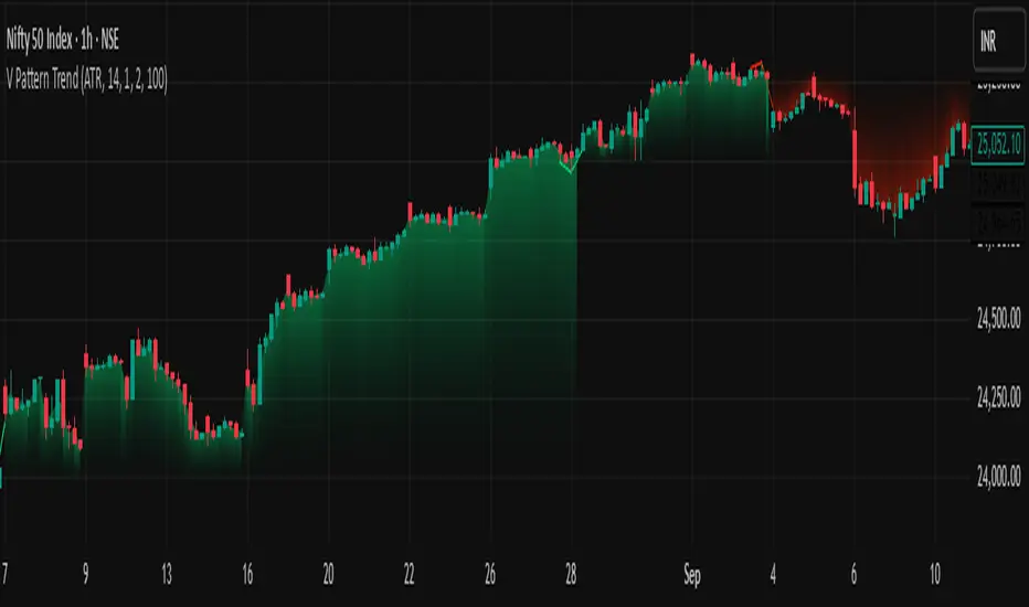
Alligator + Fractals + Divergent & Squat Bars + Signal AlertsThe indicator includes Williams Alligator, Williams Fractals, Divergent Bars, Market Facilitation Index, Highest and Lowest Bars, maximum and minimum peak of Awesome Oscillator, and signal alerts based on Bill Williams' Profitunity strategy.
MFI and Awesome Oscillator
According to the Market Facilitation Index Oscillator, the Squat bar is colored blue, all other bars are colored according to the Awesome Oscillator color, except for the Fake bars, colored with a lighter AO color. In the indicator settings, you can enable the display of "Green" bars (in the "Green Bars > Show" field). In the indicator style settings, you can disable changing the color of bars in accordance with the AO color (in the "AO bars" field), including changing the color for Fake bars (in the "Fake AO bars" field).
MFI is calculated using the formula: (high - low) / volume.
A Squat bar means that, compared to the previous bar, its MFI has decreased and at the same time its volume has increased, i.e. MFI < previous bar and volume > previous bar. A sign of a possible price reversal, so this is a particularly important signal.
A Fake bar is the opposite of a Squat bar and means that, compared to the previous bar, its MFI has increased and at the same time its volume has decreased, i.e. MFI > previous bar and volume < previous bar.
A "Green" bar means that, compared to the previous bar, its MFI has increased and at the same time its volume has increased, i.e. MFI > previous bar and volume > previous bar. A sign of trend continuation. But a more significant trend confirmation or warning of a possible reversal is the Awesome Oscillator, which measures market momentum by calculating the difference between the 5 Period and 34 Period Simple Moving Averages (SMA 5 - SMA 34) based on the midpoints of the bars (hl2). Therefore, by default, the "Green" bars and their opposite "Fade" bars are colored according to the color of the Awesome Oscillator.
According to Bill Williams' Profitunity strategy, using the Awesome Oscillator, the third Elliott wave is determined by the maximum peak of AO in the range from 100 to 140 bars. The presence of divergence between the maximum AO peak and the subsequent lower AO peak in this interval also warns of a possible correction, especially if the AO crosses the zero line between these AO peaks. Therefore, the chart additionally displays the prices of the highest and lowest bars, as well as the maximum or minimum peak of AO in the interval of 140 bars from the last bar. In the indicator settings, you can hide labels, lines, change the number of bars and any parameters for the AO indicator - method (SMA, Smoothed SMA, EMA and others), length, source (open, high, low, close, hl2 and others).
Bullish Divergent bar
🟢 A buy signal (Long) is a Bullish Divergent bar with a green circle displayed above it if such a bar simultaneously meets all of the following conditions:
The high of the bar is below all lines of the Alligator indicator.
The closing price of the bar is above its middle, i.e. close > (high + low) / 2.
The low of the bar is below the low of 2 previous bars or below the low of one previous bar, and the low of the second previous bar is a lower fractal (▼). By default, Divergent bars are not displayed, the low of which is lower than the low of only one previous bar and the low of the 2nd previous bar is not a lower fractal (▼), but you can enable the display of any Divergent bars in the indicator settings (by setting the value "no" in the " field Divergent Bars > Filtration").
The following conditions strengthen the Bullish Divergent bar signal:
The opening price of the bar, as well as the closing price, is higher than its middle, i.e. Open > (high + low) / 2.
The high of the bar is below all lines of the open Alligator indicator, i.e. the green line (Lips) is below the red line (Teeth) and the red line is below the blue line (Jaw). In this case, the color of the circle above the Bullish Divergent bar is dark green.
Squat Divergent bar.
The bar following the Bullish Divergent bar corresponds to the green color of the Awesome Oscillator.
Divergence on Awesome Oscillator.
Formation of the lower fractal (▼), in which the low of the Divergent bar is the peak of the fractal.
Bearish Divergent bar
🔴 A signal to sell (Short) is a Bearish Divergent bar under which a red circle is displayed if such a bar simultaneously meets all the following conditions:
The low of the bar is above all lines of the Alligator indicator.
The closing price of the bar is below its middle, i.e. close < (high + low) / 2.
The high of the bar is higher than the high of 2 previous bars or higher than the high of one previous bar, and the high of the second previous bar is an upper fractal (▲). By default, Divergent bars are not displayed, the high of which is higher than the high of only one previous bar and the high of the 2nd previous bar is not an upper fractal (▲), but you can enable the display of any Divergent bars in the indicator settings (by setting the value "no" in the " field Divergent Bars > Filtration").
The following conditions strengthen the Bearish Divergent bar signal:
The opening price of the bar, as well as the closing price, is below its middle, i.e. open < (high + low) / 2.
The low of the bar is above all lines of the open Alligator indicator, i.e. the green line (Lips) is above the red line (Teeth) and the red line is above the blue line (Jaw). In this case, the color of the circle under the Bearish Divergent bar is dark red.
Squat Divergent bar.
The bar following the Bearish Divergent bar corresponds to the red color of the Awesome Oscillator.
Divergence on Awesome Oscillator.
Formation of the upper fractal (▲), in which the high of the Divergent bar is the peak of the fractal.
Alligator lines crossing
Bars crossing the green line (Lips) of the open Alligator indicator is the first warning of a possible correction (price rollback) if one of the following conditions is met:
If the bar closed below the Lips line, which is above the Teeth line, and the Teeth line is above the Jaw line, while the closing price of the previous bar is above the Lips line.
If the bar closed above the Lips line, which is below the Teeth line, and the Teeth line is below the Jaw line, while the closing price of the previous bar is below the Lips line.
The intersection of all open Alligator lines by bars is a sign of a deep correction and a warning of a possible trend change.
Frequent intersection of Alligator lines with each other is a sign of a sideways trend (flat).
Signal Alerts
To receive notifications about signals when creating an alert, you must select the condition "Any alert() function is call", in which case notifications will arrive in the following format:
D — timeframe, for example: D, 4H, 15m.
🟢 BDB⎾ - a signal for a Bullish Divergent bar to buy (Long), triggers once after the bar closes and includes additional signals:
/// — if Alligator is open.
⏉ — if the opening price of the bar, as well as the closing price, is above its middle.
+ Squat 🔷 - Squat bar or + Green ↑ - "Green" bar or + Fake ↓ - Fake bar.
+ AO 🟩 - if after the Divergent bar closes, the oscillator color change for the next bar corresponds the green color of the Awesome Oscillator. ┴/┬ — AO above/below the zero line. ∇ — if there is divergence on AO in the interval of 140 bars from the last bar.
🔴 BDB⎿ - a signal for a Bearish Divergent bar to sell (Short), triggers once after the bar closes and includes additional signals:
/// — if Alligator is open.
⏊ — if the opening price of the bar, as well as the closing price, is below its middle.
+ Squat 🔷 - Squat bar or + Green ↑ - "Green" bar or + Fake ↓ - Fake bar.
+ AO 🟥 - if after the Divergent bar closes, the oscillator color change for the next bar corresponds to the red color of the Awesome Oscillator. ┴/┬ — AO above/below the zero line. ∇ — if there is divergence on AO in the interval of 140 bars from the last bar.
Alert for bars crossing the green line (Lips) of the open Alligator indicator (can be disabled in the indicator settings in the "Alligator > Enable crossing lips alerts" field):
🔴 Crossing Lips ↓ - if the bar closed below the Lips line, which is above than the other lines, while the closing price of the previous bar is above the Lips line.
🟢 Crossing Lips ↑ - if the bar closed above the Lips line, which is below the other lines, while the closing price of the previous bar is below the Lips line.
The fractal signal is triggered after the second bar closes, completing the formation of the fractal, if alerts about fractals are enabled in the indicator settings (the "Fractals > Enable alerts" field):
🟢 Fractal ▲ - upper (Bearish) fractal.
🔴 Fractal ▼ — lower (Bullish) fractal.
⚪️ Fractal ▲/▼ - both upper and lower fractal.
↳ (H=high - L=low) = difference.
If you redirect notifications to a webhook URL, for example, to a Telegram bot, then you need to set the notification template for the webhook in the indicator settings in the "Webhook > Message" field (contains a tooltip with an example), in which you just need to specify the text {{message}}, which will be automatically replaced with the alert text with a ticker and a link to TradingView.
‼️ A signal is not a call to action, but only a reason to analyze the chart to make a decision based on the rules of your strategy.
***
Индикатор включает в себя Williams Alligator, Williams Fractals, Дивергентные бары, Market Facilitation Index, самый высокий и самый низкий бары, максимальный и минимальный пик Awesome Oscillator, а также оповещения о сигналах на основе стратегии Profitunity Билла Вильямса.
MFI и Awesome Oscillator
В соответствии с осциллятором Market Facilitation Index Приседающий бар окрашен в синий цвет, все остальные бары окрашены в соответствии с цветом Awesome Oscillator, кроме Фальшивых баров, которые окрашены более светлым цветом AO. В настройках индикатора вы можете включить отображение "Зеленых" баров (в поле "Green Bars > Show"). В настройках стиля индикатора вы можете выключить изменение цвета баров в соответствии с цветом AO (в поле "AO bars"), в том числе изменить цвет для Фальшивых баров (в поле "Fake AO bars").
MFI рассчитывается по формуле: (high - low) / volume.
Приседающий бар означает, что по сравнению с предыдущим баром его MFI снизился и в тоже время вырос его объем, т.е. MFI < предыдущего бара и объем > предыдущего бара. Признак возможного разворота цены, поэтому это особенно важный сигнал.
Фальшивый бар является противоположностью Приседающему бару и означает, что по сравнению с предыдущим баром его MFI увеличился и в тоже время снизился его объем, т.е. MFI > предыдущего бара и объем < предыдущего бара.
"Зеленый" бар означает, что по сравнению с предыдущим баром его MFI увеличился и в тоже время вырос его объем, т.е. MFI > предыдущего бара и объем > предыдущего бара. Признак продолжения тренда. Но более значимым подтверждением тренда или предупреждением о возможном развороте является Awesome Oscillator, который измеряет движущую силу рынка путем вычисления разницы между 5 Периодной и 34 Периодной Простыми Скользящими Средними (SMA 5 - SMA 34) по средним точкам баров (hl2). Поэтому по умолчанию "Зеленые" бары и противоположные им "Увядающие" бары окрашены в соответствии с цветом Awesome Oscillator.
По стратегии Profitunity Билла Вильямса с помощью осциллятора Awesome Oscillator определяется третья волна Эллиота по максимальному пику AO в интервале от 100 до 140 баров. Наличие дивергенции между максимальным пиком AO и следующим за ним более низким пиком AO в этом интервале также предупреждает о возможной коррекции, особенно если AO переходит через нулевую линию между этими пиками AO. Поэтому на графике дополнительно отображаются цены самого высокого и самого низкого баров, а также максимальный или минимальный пик АО в интервале 140 баров от последнего бара. В настройках индикатора вы можете скрыть метки, линии, изменить количество баров и любые параметры для индикатора AO – метод (SMA, Smoothed SMA, EMA и другие), длину, источник (open, high, low, close, hl2 и другие).
Бычий Дивергентный бар
🟢 Сигналом на покупку (Long) является Бычий Дивергентный бар над которым отображается зеленый круг, если такой бар соответствует одновременно всем следующим условиям:
Максимум бара ниже всех линий индикатора Alligator.
Цена закрытия бара выше его середины, т.е. close > (high + low) / 2.
Минимум бара ниже минимума 2-х предыдущих баров или ниже минимума одного предыдущего бара, а минимум второго предыдущего бара является нижним фракталом (▼). По умолчанию не отображаются Дивергентные бары, минимум которых ниже минимума только одного предыдущего бара и минимум 2-го предыдущего бара не является нижним фракталом (▼), но вы можете включить отображение любых Дивергентных баров в настройках индикатора (установив значение "no" в поле "Divergent Bars > Filtration").
Усилением сигнала Бычьего Дивергентного бара являются следующие условия:
Цена открытия бара, как и цена закрытия, выше его середины, т.е. Open > (high + low) / 2.
Максимум бара ниже всех линий открытого индикатора Alligator, т.е. зеленая линия (Lips) ниже красной линии (Teeth) и красная линия ниже синей линии (Jaw). В этом случае цвет круга над Бычьим Дивергентным баром окрашен в темно-зеленый цвет.
Приседающий Дивергентный бар.
Бар, следующий за Бычьим Дивергентным баром, соответствует зеленому цвету Awesome Oscillator.
Дивергенция на Awesome Oscillator.
Образование нижнего фрактала (▼), у которого минимум Дивергентного бара является пиком фрактала.
Медвежий Дивергентный бар
🔴 Сигналом на продажу (Short) является Медвежий Дивергентный бар под которым отображается красный круг, если такой бар соответствует одновременно всем следующим условиям:
Минимум бара выше всех линий индикатора Alligator.
Цена закрытия бара ниже его середины, т.е. close < (high + low) / 2.
Максимум бара выше маскимума 2-х предыдущих баров или выше максимума одного предыдущего бара, а максимум второго предыдущего бара является верхним фракталом (▲). По умолчанию не отображаются Дивергентные бары, максимум которых выше максимума только одного предыдущего бара и максимум 2-го предыдущего бара не является верхним фракталом (▲), но вы можете включить отображение любых Дивергентных баров в настройках индикатора (установив значение "no" в поле "Divergent Bars > Filtration").
Усилением сигнала Медвежьего Дивергентного бара являются следующие условия:
Цена открытия бара, как и цена закрытия, ниже его середины, т.е. open < (high + low) / 2.
Минимум бара выше всех линий открытого индикатора Alligator, т.е. зеленая линия (Lips) выше красной линии (Teeth) и красная линия выше синей линии (Jaw). В этом случае цвет круга под Медвежьим Дивергентным Баром окрашен в темно-красный цвет.
Приседающий Дивергентный бар.
Бар, следующий за Медвежьим Дивергентным баром, соответствует красному цвету Awesome Oscillator.
Дивергенция на Awesome Oscillator.
Образование верхнего фрактала (▲), у которого максимум Дивергентного бара является пиком фрактала.
Пересечение линий Alligator
Пересечение барами зеленой линии (Lips) открытого индикатора Alligator является первым предупреждением о возможной коррекции (откате цены) при выполнении одного из следующих условий:
Если бар закрылся ниже линии Lips, которая выше линии Teeth, а линия Teeth выше линии Jaw, при этом цена закрытия предыдущего бара находится выше линии Lips.
Если бар закрылся выше линии Lips, которая ниже линии Teeth, а линия Teeth ниже линии Jaw, при этом цена закрытия предыдущего бара находится ниже линии Lips.
Пересечение барами всех линий открытого Alligator является признаком глубокой коррекции и предупреждением о возможной смене тренда.
Частое пересечение линий Alligator между собой является признаком бокового тренда (флэт).
Оповещения о сигналах
Для получения уведомлений о сигналах при создании оповещения необходимо выбрать условие "При любом вызове функции alert()", в таком случае уведомления будут приходить в следующем формате:
D — таймфрейм, например: D, 4H, 15m.
🟢 BDB⎾ — сигнал Бычьего Дивергентного бара на покупку (Long), срабатывает один раз после закрытия бара и включает дополнительные сигналы:
/// — если Alligator открыт.
⏉ — если цена открытия бара, как и цена закрытия, выше его середины.
+ Squat 🔷 — Приседающий бар или + Green ↑ — "Зеленый" бар или + Fake ↓ — Фальшивый бар.
+ AO 🟩 — если после закрытия Дивергентного бара, изменение цвета осциллятора для следующего бара соответствует зеленому цвету Awesome Oscillator. ┴/┬ — AO выше/ниже нулевой линии. ∇ — если есть дивергенция на AO в интервале 140 баров от последнего бара.
🔴 BDB⎿ — сигнал Медвежьего Дивергентного бара на продажу (Short), срабатывает один раз после закрытия бара и включает дополнительные сигналы:
/// — если Alligator открыт.
⏊ — если цена открытия бара, как и цена закрытия, ниже его середины.
+ Squat 🔷 — Приседающий бар или + Green ↑ — "Зеленый" бар или + Fake ↓ — Фальшивый бар.
+ AO 🟥 — если после закрытия Дивергентного бара, изменение цвета осциллятора для следующего бара соответствует красному цвету Awesome Oscillator. ┴/┬ — AO выше/ниже нулевой линии. ∇ — если есть дивергенция на AO в интервале 140 баров от последнего бара.
Сигнал пересечения барами зеленой линии (Lips) открытого индикатора Alligator (можно отключить в настройках индикатора в поле "Alligator > Enable crossing lips alerts"):
🔴 Crossing Lips ↓ — если бар закрылся ниже линии Lips, которая выше остальных линий, при этом цена закрытия предыдущего бара находится выше линии Lips.
🟢 Crossing Lips ↑ — если бар закрылся выше линии Lips, которая ниже остальных линий, при этом цена закрытия предыдущего бара находится ниже линии Lips.
Сигнал фрактала срабатывает после закрытия второго бара, завершающего формирование фрактала, если оповещения о фракталах включены в настройках индикатора (поле "Fractals > Enable alerts"):
🟢 Fractal ▲ — верхний (Медвежий) фрактал.
🔴 Fractal ▼ — нижний (Бычий) фрактал.
⚪️ Fractal ▲/▼ — одновременно верхний и нижний фрактал.
↳ (H=high - L=low) = разница.
Если вы перенаправляете оповещения на URL вебхука, например, в бота Telegram, то вам необходимо установить шаблон оповещения для вебхука в настройках индикатора в поле "Webhook > Message" (содержит подсказку с примером), в котором в качестве текста сообщения достаточно указать текст {{message}}, который будет автоматически заменен на текст оповещения с тикером и ссылкой на TradingView.
‼️ Сигнал — это не призыв к действию, а лишь повод проанализировать график для принятия решения на основе правил вашей стратегии.

YD_Divergence_RSI+CMFThe ‘YD_Divergence_RSI+CMF’ indicator can find divergence using RSI (Relative Strength Index) and CMF (Chaikin Money Flow) indicators.
📌 Key functions
1. Search pivot high and pivot low points in a certain length of price.
2. Connect pivot high to pivot high , pivot low to pivot low , forming two standards for divergence in result.
The marker then plots only the higher high, lower low lines.
(higher low and lower high in prices are referred to hidden divergence, which are not considered in this indicator)
3. Compare the two standards with RSI and CMF indicators, send an alert if there is a divergence. As a result, the indicator will find four combination of divergence.
A. Higher high price / Lower RSI (Bearish RSI Divergence)
B. Lower low price / Higher RSI (Bullish RSI Divergence)
C. Higher high price / Lower CMF (Bearish CMF Divergence)
D. Lower low price / Higher CMF (Bullish CMF Divergence)
📌 Details
Developing the indicators, we put a lot of effort in making a customizable and user-friendly interface.
#1. Pivot Setting
Users can set the length to find the pivot high / pivot low in ‘Pivot Settings – Pivot Length.’
Increased pivot Length takes more candles to interpret the chart but reduce false signals since the it uses only the most certain pivot high / pivot low values. Obviously, decreased pivot length will act the opposite.
Users can choose whether to use ‘High/Low’ or ‘Close’ in ‘Pivot Reference’ to set the swing point of prices.
Users can also choose whether to display the pivot high / pivot low marker on the chart.
#2 RSI & CMF Settings
Users can adjust the length of RSI & CMF separately. (The default values are set to 14 and 20 each.)
#3 Label Setting
Users can adjust the text displayed on the chart label. (The default values is set to ‘Bullish / Bearish’, ‘RSI/CMF’, ‘Divergence’.)
Users can reduce the length of text label or simply turn the label off. Just click the ‘Bull/Bear’ or ‘None’ button. ‘Divergence’ works the same.
Users can decide whether to display the ‘Divergence Line and Label’, set custom settings for the label and line. (color, thickness, style, etc)
📌 Alert
Alert are provided as a combination of the chart's symbol and the set label text. For example,
‘BINANCE:BTCUSDT.P, Bullish RSI Divergence’
====================================================
"YD_Divergence_RSI+CMF" 지표 는 RSI와 CMF 지표를 이용해서 Divergence 를 찾아낼 수 있습니다.
📌 주요 기능
1. 정해진 가격 움직임 안에서 pivot high와 pivot low 포인트 를 찾아냅니다.
2. Pivot high로만 이어진 라인과, Pivot low로만 이어진 두 라인을 작도한 뒤 divergence의 기준으로 삼습니다.
이 지표에서는 normal divergence만 사용하기 때문에 차트에 higher high와 lower low만 표기 합니다.
(higher low와 lower high는 hidden divergence로 정의되며, 이 지표에서는 다루지 않습니다.
3. 두 기준선과 RSI, CMF 지표를 각각 비교하고, 결과적으로 4개의 조합을 구할 수 있습니다.
A. Higher high price / Lower RSI (Bearish RSI Divergence)
B. Lower low price / Higher RSI (Bullish RSI Divergence)
C. Higher high price / Lower CMF (Bearish CMF Divergence)
D. Lower low price / Higher CMF (Bullish CMF Divergence)
📌 세부 사항
지표를 개발하며 사용자들이 원하는 방향으로 지표를 설정할 수 있게 작업에 많은 공을 들였습니다. 굉장히 다양한 옵션을 선택할 수 있으며, 원하는 방식으로 지표를 사용할 수 있습니다.
#1 Pivot Setting
Pivot setting에서는 Pivot Length를 변경할 수 있습니다.
Pivot Length를 늘릴 경우, 보다 확실한 Swing High와 Swing Low만을 사용하게 되므로, False signal이 줄어들 수 있습니다. 하지만 Swing High/ Low를 판정하는 데에 더 긴 시간이 걸리게 되므로, Signal이 다소 늦게 발생하는 단점이 생기게 됩니다.
Pivot Length를 줄일 경우, 반대로 Swing High/Low의 판정이 더 빨리 일어나기 때문에, Signal을 거래에 이용하기는 좋을 수 있습니다. 다만, Swing High와 Low가 훨씬 더 잦은 빈도로 발생하기 때문에 False Signal을 줄 가능성이 높아집니다.
Pivot Reference에서는 가격의 Swing Point를 설정함에 있어, High/Low(고가/저가)를 이용할 지 Close (종가)를 이용할 지 선택할 수 있습니다.
Pivot High/Low Marker를 선택할 경우 Pivot High/ Low에 Marker가 찍히게 됩니다.
#2 RSI와 CMF Setting
RSI와 CMF Setting에서는 RSI와 CMF의 길이를 각각 설정할 수 있습니다. 기본값은 14와 20으로 설정되어 있습니다.
#3 Label Setting
Label Setting에서는 Label에 표시되는 글자를 선택할 수 있습니다.
기본값은 "Bullish / Bearish", "RSI/CMF", "Divergence"로 선택되어 있으며, 너무 길다고 느껴질 경우 "Bull/Bear" 혹은 "None"을 클릭하여 길이를 줄일 수 있습니다. 마찬가지로 Divergence의 경우도 생략이 가능합니다.
하단에서는 Divergence Line과 Label을 켜고 끌 수 있으며, 선의 색깔, 굵기, 종류, 그리고 Label의 색깔, 크기, 종류를 선택할 수 있습니다. Label의 Text 색 역시 변경이 가능합니다.
📌 얼러트
얼러트는 자신이 설정한 차트의 심볼과 Label의 문구의 조합으로 제공되며 예를 들면 다음과 같습니다.
"BINANCE:BTCUSDT.P, Bullish RSI Divergence"

Larry Williams Strategies IndicatorThis indicator is a trend following indicator. It plots some of the trend following strategies described by Larry Williams in his book 'Long Term Secrets to Short Term Trading'. Below are types of trend following strategies you can trade using this indicator. These are notes taken directly from Larry Williams' book.
Short Term Low Strategy
Short Term Low - Any daily low with higher lows on each side of it.
Intermediate Term Low – Any short term low with higher short term lows on each side of it.
Long Term Low – Any intermediate term low with higher intermediate term lows on each side of it.
Conceptual pattern for best buying opportunity is when forming an intermediate term low higher than the last intermediate term low.
This setup can be used on all time frames. However since Larry Williams usually trades the daily chart, the daily chart is probably the best timeframe to trade using this strategy.
Entry point – High of the day that has a higher high on the right side of it.
(My interpretation: price crossing above the high of the previous day is the buy signal)
Target – Markets have a strong tendency to rally above the last intermediate term high by the same amount it moved from the last intermediate term high to the lowest point prior to advancing to new highs.
Trailing Stop – Set stop to most recent short term low, move up as new short term lows are formed. Can also use formation of next intermediate term high as an exit point.
A 'run' to the upside is over when price fails to move higher the next day and falls below the prior day's low.
Short Term High Strategy
Short Term High - Any daily high with lower highs on each side of it.
Intermediate Term High – Any short term high with lower short term highs on each side of it.
Long Term High – Any intermediate term high with lower intermediate term highs on each side of it.
Conceptual pattern for best selling opportunity is when forming an intermediate term high lower than the last intermediate term high.
This setup can be used on all time frames. However since Larry Williams usually trades the daily chart, the daily chart is probably the best timeframe to trade using this strategy.
Entry point – Low of the day that has a lower low on the right side of it.
(My interpretation: price crossing below the low of the previous day is the sell short signal)
Target – Markets have a strong tendency to fall below the last intermediate term low by the same amount it moved from the last intermediate term low to the highest point prior to declining to new lows.
Trailing Stop – Set stop to most recent short term high, move down as new short term highs are formed. Can also use formation of next intermediate term low as an exit point.
A 'run' to the downside is over when price fails to move lower the next day and rises above the prior day's high.
Trend Reversals
A trend change from down to up occurs when a short term high is exceeded on the upside, a trend change from up to down is identified by price going below the most recent low.
Can take these signals to make trades, but it is best to filter them with a confirmation or edge such as Trading Day of the Week, Trading Day of the Month, trendlines, etc. to cut down on false signals.
Three Bar High/Low System
Calculate a three bar moving average of the highs and a three bar moving average of the lows.
Strategy is to buy at the at the price of the three bar moving average of the lows - if the trend is positive according to the swing point trend identification technique - and take profits at the three bar moving average of the highs.
Selling is just the opposite. Sell short at the three bar moving average of the highs and take profits at the three bar moving average of the lows, using the trend identification technique above for confirmation.
This strategy can work on any timeframe, but was described as a daytrading system by Larry Williams.

VV Moving Average Convergence Divergence # VMACDv3 - Volume-Weighted MACD with A/D Divergence Detection
## Overview
**VMACDv3** (Volume-Weighted Moving Average Convergence Divergence Version 3) is a momentum indicator that applies volume-weighting to traditional MACD calculations on price, while using the Accumulation/Distribution (A/D) line for divergence detection. This hybrid approach combines volume-weighted price momentum with volume distribution analysis for comprehensive market insight.
## Key Features
- **Volume-Weighted Price MACD**: Traditional MACD calculation on price but weighted by volume for earlier signals
- **A/D Divergence Detection**: Identifies when A/D trend diverges from MACD momentum
- **Volume Strength Filtering**: Distinguishes high-volume confirmations from low-volume noise
- **Color-Coded Histogram**: 4-color system showing momentum direction and volume strength
- **Real-Time Alerts**: Background colors and alert conditions for bullish/bearish divergences
## Difference from ACCDv3
| Aspect | VMACDv3 | ACCDv3 |
|--------|---------|---------|
| **MACD Input** | **Price (Close)** | **A/D Line** |
| **Volume Weighting** | Applied to price | Applied to A/D line |
| **Primary Signal** | Volume-weighted price momentum | Volume distribution momentum |
| **Use Case** | Price momentum with volume confirmation | Volume flow and accumulation/distribution |
| **Sensitivity** | More responsive to price changes | More responsive to volume patterns |
| **Best For** | Trend following, breakouts | Volume analysis, smart money tracking |
**Key Insight**: VMACDv3 shows *where price is going* with volume weight, while ACCDv3 shows *where volume is accumulating/distributing*.
## Components
### 1. Volume-Weighted MACD on Price
Unlike standard MACD that uses simple price EMAs, VMACDv3 weights each price by its corresponding volume:
```
Fast Line = EMA(Price × Volume, 12) / EMA(Volume, 12)
Slow Line = EMA(Price × Volume, 26) / EMA(Volume, 26)
MACD = Fast Line - Slow Line
```
**Benefits of Volume Weighting**:
- High-volume price movements have greater impact
- Filters out low-volume noise and false moves
- Provides earlier trend change signals
- Better reflects institutional activity
### 2. Accumulation/Distribution (A/D) Line
Used for divergence detection, measuring buying/selling pressure:
```
A/D = Σ ((2 × Close - Low - High) / (High - Low)) × Volume
```
- **Rising A/D**: Accumulation (buying pressure)
- **Falling A/D**: Distribution (selling pressure)
- **Doji Handling**: When High = Low, contribution is zero
### 3. Signal Lines
- **MACD Line** (Blue, #2962FF): The fast-slow difference showing momentum
- **Signal Line** (Orange, #FF6D00): EMA or SMA smoothing of MACD
- **Zero Line**: Reference for bullish (above) vs bearish (below) bias
### 4. Histogram Color System
The histogram uses 4 distinct colors based on **direction** and **volume strength**:
| Condition | Color | Meaning |
|-----------|-------|---------|
| Rising + High Volume | **Dark Green** (#1B5E20) | Strong bullish momentum with volume confirmation |
| Rising + Low Volume | **Light Teal** (#26A69A) | Bullish momentum but weak volume (less reliable) |
| Falling + High Volume | **Dark Red** (#B71C1C) | Strong bearish momentum with volume confirmation |
| Falling + Low Volume | **Light Pink** (#FFCDD2) | Bearish momentum but weak volume (less reliable) |
Additional shading:
- **Light Cyan** (#B2DFDB): Positive but not rising (momentum stalling)
- **Bright Red** (#FF5252): Negative and accelerating down
### 5. Divergence Detection
VMACDv3 compares A/D trend against volume-weighted price MACD:
#### Bullish Divergence (Green Background)
- **Condition**: A/D is trending up BUT MACD is negative and trending down
- **Interpretation**: Volume is accumulating while price momentum appears weak
- **Signal**: Smart money accumulation, potential bullish reversal
- **Action**: Look for long entries, especially at support levels
#### Bearish Divergence (Red Background)
- **Condition**: A/D is trending down BUT MACD is positive and trending up
- **Interpretation**: Volume is distributing while price momentum appears strong
- **Signal**: Smart money distribution, potential bearish reversal
- **Action**: Consider exits, avoid new longs, watch for breakdown
## Parameters
| Parameter | Default | Range | Description |
|-----------|---------|-------|-------------|
| **Source** | Close | OHLC/HLC3/etc | Price source for MACD calculation |
| **Fast Length** | 12 | 1-50 | Period for fast EMA (shorter = more sensitive) |
| **Slow Length** | 26 | 1-100 | Period for slow EMA (longer = smoother) |
| **Signal Smoothing** | 9 | 1-50 | Period for signal line (MACD smoothing) |
| **Signal Line MA Type** | EMA | SMA/EMA | Moving average type for signal calculation |
| **Volume MA Length** | 20 | 5-100 | Period for volume average (strength filter) |
## Usage Guide
### Reading the Indicator
1. **MACD Lines (Blue & Orange)**
- **Blue Line (MACD)**: Volume-weighted price momentum
- **Orange Line (Signal)**: Smoothed trend of MACD
- **Crossovers**: Blue crosses above orange = bullish, below = bearish
- **Distance**: Wider gap = stronger momentum
- **Zero Line Position**: Above = bullish bias, below = bearish bias
2. **Histogram Colors**
- **Dark Green (#1B5E20)**: Strong bullish move with high volume - **most reliable buy signal**
- **Light Teal (#26A69A)**: Bullish but low volume - wait for confirmation
- **Dark Red (#B71C1C)**: Strong bearish move with high volume - **most reliable sell signal**
- **Light Pink (#FFCDD2)**: Bearish but low volume - may be temporary dip
3. **Background Divergence Alerts**
- **Green Background**: A/D accumulating while price weak - potential bottom
- **Red Background**: A/D distributing while price strong - potential top
- Most powerful at key support/resistance levels
### Trading Strategies
#### Strategy 1: Volume-Confirmed Trend Following
1. Wait for MACD to cross above zero line
2. Look for **dark green** histogram bars (high volume confirmation)
3. Enter long on second consecutive dark green bar
4. Hold while histogram remains green
5. Exit when histogram turns light green or red appears
6. Set stop below recent swing low
**Example**:
```
Price: 26,400 → 26,450 (rising)
MACD: -50 → +20 (crosses zero)
Histogram: Light teal → Dark green → Dark green
Volume: 50k → 75k → 90k (increasing)
```
#### Strategy 2: Divergence Reversal Trading
1. Identify divergence background (green = bullish, red = bearish)
2. Confirm with price structure (support/resistance, chart patterns)
3. Wait for MACD to cross signal line in divergence direction
4. Enter on first **dark colored** histogram bar after divergence
5. Set stop beyond divergence area
6. Target previous swing high/low
**Example - Bullish Divergence**:
```
Price: Making lower lows (26,350 → 26,300 → 26,250)
A/D: Rising (accumulation)
MACD: Below zero but starting to curve up
Background: Green shading appears
Entry: MACD crosses signal line + dark green bar
Stop: Below 26,230
Target: 26,450 (previous high)
```
#### Strategy 3: Momentum Scalping
1. Trade only in direction of MACD zero line (above = long, below = short)
2. Enter on dark colored bars only
3. Exit on first light colored bar or opposite color
4. Quick in and out (1-5 minute holds)
5. Tight stops (0.2-0.5% depending on instrument)
#### Strategy 4: Histogram Pattern Trading
**V-Bottom Reversal (Bullish)**:
- Red histogram bars start rising (becoming less negative)
- Forms "V" shape at the bottom
- Transitions to light red → light teal → **dark green**
- Entry: First dark green bar
- Signal: Momentum reversal with volume
**Λ-Top Reversal (Bearish)**:
- Green histogram bars start falling (becoming less positive)
- Forms inverted "V" at the top
- Transitions to light green → light pink → **dark red**
- Entry: First dark red bar
- Signal: Momentum exhaustion with volume
### Multi-Timeframe Analysis
**Recommended Approach**:
1. **Higher Timeframe (15m/1h)**: Identify overall trend direction
2. **Trading Timeframe (5m)**: Time entries using VMACDv3 signals
3. **Lower Timeframe (1m)**: Fine-tune entry prices
**Example Setup**:
```
15-minute: MACD above zero (bullish bias)
5-minute: Dark green histogram appears after pullback
1-minute: Enter on break of recent high with volume
```
### Volume Strength Interpretation
The volume filter compares current volume to 20-period average:
- **Volume > Average**: Dark colors (green/red) - high confidence signals
- **Volume < Average**: Light colors (teal/pink) - lower confidence signals
**Trading Rules**:
- ✓ **Aggressive**: Take all dark colored signals
- ✓ **Conservative**: Only take dark colors that follow 2+ light colors of same type
- ✗ **Avoid**: Trading light colored signals during high volatility
- ✗ **Avoid**: Ignoring volume context during news events
## Technical Details
### Volume-Weighted Calculation
```pine
// Volume-weighted fast EMA
fast_ma = ta.ema(src * volume, fast_length) / ta.ema(volume, fast_length)
// Volume-weighted slow EMA
slow_ma = ta.ema(src * volume, slow_length) / ta.ema(volume, slow_length)
// MACD is the difference
macd = fast_ma - slow_ma
// Signal line smoothing
signal = ta.ema(macd, signal_length) // or ta.sma() if SMA selected
// Histogram
hist = macd - signal
```
### Divergence Detection Logic
```pine
// A/D trending up if above its 5-period SMA
ad_trend = ad > ta.sma(ad, 5)
// MACD trending up if above zero
macd_trend = macd > 0
// Divergence when trends oppose each other
divergence = ad_trend != macd_trend
// Specific conditions for alerts
bullish_divergence = ad_trend and not macd_trend and macd < 0
bearish_divergence = not ad_trend and macd_trend and macd > 0
```
### Histogram Coloring Logic
```pine
hist_color = (hist >= 0
? (hist < hist
? (vol_strength ? #1B5E20 : #26A69A) // Rising: dark/light green
: #B2DFDB) // Positive but falling: cyan
: (hist < hist
? (vol_strength ? #B71C1C : #FFCDD2) // Rising (less negative): dark/light red
: #FF5252)) // Falling more: bright red
```
## Alerts
Built-in alert conditions for divergence detection:
### Bullish Divergence Alert
- **Trigger**: A/D trending up, MACD negative and trending down
- **Message**: "Bullish Divergence: A/D trending up but MACD trending down"
- **Use Case**: Potential reversal or continuation after pullback
- **Action**: Look for long entry setups
### Bearish Divergence Alert
- **Trigger**: A/D trending down, MACD positive and trending up
- **Message**: "Bearish Divergence: A/D trending down but MACD trending up"
- **Use Case**: Potential top or trend reversal
- **Action**: Consider exits or short entries
### Setting Up Alerts
1. Click "Create Alert" in TradingView
2. Condition: Select "VMACDv3"
3. Choose alert type: "Bullish Divergence" or "Bearish Divergence"
4. Configure: Email, SMS, webhook, or popup
5. Set frequency: "Once Per Bar Close" recommended
## Comparison Tables
### VMACDv3 vs Standard MACD
| Feature | Standard MACD | VMACDv3 |
|---------|---------------|---------|
| **Price Weighting** | Equal weight all bars | Volume-weighted |
| **Sensitivity** | Fixed | Adaptive to volume |
| **False Signals** | More during low volume | Fewer (volume filter) |
| **Divergence** | Price vs MACD | A/D vs MACD |
| **Volume Analysis** | None | Built-in |
| **Color System** | 2 colors | 4+ colors |
| **Best For** | Simple trend following | Volume-confirmed trading |
### VMACDv3 vs ACCDv3
| Aspect | VMACDv3 | ACCDv3 |
|--------|---------|--------|
| **Focus** | Price momentum | Volume distribution |
| **Reactivity** | Faster to price moves | Faster to volume shifts |
| **Best Markets** | Trending, breakouts | Accumulation/distribution phases |
| **Signal Type** | Where price + volume going | Where smart money positioning |
| **Divergence Meaning** | Volume vs price disagreement | A/D vs momentum disagreement |
| **Use Together?** | ✓ Yes, complementary | ✓ Yes, different perspectives |
## Example Trading Scenarios
### Scenario 1: Strong Bullish Breakout
```
Time: 9:30 AM (market open)
Price: Breaks above 26,400 resistance
MACD: Crosses above zero line
Histogram: Dark green bars (#1B5E20)
Volume: 2x average (150k vs 75k avg)
A/D: Rising (no divergence)
Action: Enter long at 26,405
Stop: 26,380 (below breakout)
Target 1: 26,450 (risk:reward 1:2)
Target 2: 26,500 (risk:reward 1:4)
Result: High probability setup with volume confirmation
```
### Scenario 2: False Breakout (Avoided)
```
Time: 2:30 PM (slow period)
Price: Breaks above 26,400 resistance
MACD: Slightly positive
Histogram: Light teal bars (#26A69A)
Volume: 0.5x average (40k vs 75k avg)
A/D: Flat/declining
Action: Avoid trade
Reason: Low volume, no conviction, potential false breakout
Outcome: Price reverses back below 26,400 within 10 minutes
Saved: Avoided losing trade due to volume filter
```
### Scenario 3: Bullish Divergence Bottom
```
Time: 11:00 AM
Price: Making lower lows (26,350 → 26,300 → 26,280)
MACD: Below zero but curving upward
Histogram: Red bars getting shorter (V-bottom forming)
Background: Green shading (divergence alert)
A/D: Rising despite price falling
Volume: Increasing on down bars
Setup:
1. Divergence appears at 26,280 (green background)
2. Wait for MACD to cross signal line
3. First dark green bar appears at 26,290
4. Enter long: 26,295 (next bar open)
5. Stop: 26,265 (below divergence low)
6. Target: 26,350 (previous swing high)
Result: +55 points (30 point risk, 1.8:1 reward)
Key: Divergence + volume confirmation = high probability reversal
```
### Scenario 4: Bearish Divergence Top
```
Time: 1:45 PM
Price: Making higher highs (26,500 → 26,520 → 26,540)
MACD: Positive but flattening
Histogram: Green bars getting shorter (Λ-top forming)
Background: Red shading (bearish divergence)
A/D: Declining despite rising price
Volume: Decreasing on up bars
Setup:
1. Bearish divergence at 26,540 (red background)
2. MACD crosses below signal line
3. First dark red bar appears at 26,535
4. Enter short: 26,530
5. Stop: 26,555 (above divergence high)
6. Target: 26,475 (support level)
Result: +55 points (25 point risk, 2.2:1 reward)
Key: Distribution while price rising = smart money exiting
```
### Scenario 5: V-Bottom Reversal
```
Downtrend in progress
MACD: Deep below zero (-150)
Histogram: Series of dark red bars
Pattern Development:
Bar 1: Dark red, hist = -80, falling
Bar 2: Dark red, hist = -95, falling
Bar 3: Dark red, hist = -100, falling (extreme)
Bar 4: Light pink, hist = -98, rising!
Bar 5: Light pink, hist = -90, rising
Bar 6: Light teal, hist = -75, rising (crosses to positive momentum)
Bar 7: Dark green, hist = -55, rising + volume
Action: Enter long on Bar 7
Reason: V-bottom confirmed with volume
Stop: Below Bar 3 low
Target: Zero line on histogram (mean reversion)
```
## Best Practices
### Entry Rules
✓ **Wait for dark colors**: High-volume confirmation is key
✓ **Confirm divergences**: Use with price support/resistance
✓ **Trade with zero line**: Long above, short below for best odds
✓ **Multiple timeframes**: Align 1m, 5m, 15m signals
✓ **Watch for patterns**: V-bottoms and Λ-tops are reliable
### Exit Rules
✓ **Partial profits**: Take 50% at first target
✓ **Trail stops**: Use histogram color changes
✓ **Respect signals**: Exit on opposite dark color
✓ **Time stops**: Close positions before major news
✓ **End of day**: Square up before close
### Avoid
✗ **Don't chase light colors**: Low volume = low confidence
✗ **Don't ignore divergence**: Early warning system
✗ **Don't overtrade**: Wait for clear setups
✗ **Don't fight the trend**: Zero line dictates bias
✗ **Don't skip stops**: Always use risk management
## Risk Management
### Position Sizing
- **Dark green/red signals**: 1-2% account risk
- **Light signals**: 0.5% account risk or skip
- **Divergence plays**: 1% account risk (higher uncertainty)
- **Multiple confirmations**: Up to 2% account risk
### Stop Loss Placement
- **Trend trades**: Below/above recent swing (20-30 points typical)
- **Breakout trades**: Below/above breakout level (15-25 points)
- **Divergence trades**: Beyond divergence extreme (25-40 points)
- **Scalp trades**: Tight stops at 10-15 points
### Profit Targets
- **Minimum**: 1.5:1 reward to risk ratio
- **Scalps**: 15-25 points (quick in/out)
- **Swing**: 50-100 points (hold through pullbacks)
- **Runners**: Trail with histogram color changes
## Timeframe Recommendations
| Timeframe | Trading Style | Typical Hold | Advantages | Challenges |
|-----------|---------------|--------------|------------|------------|
| **1-minute** | Scalping | 1-5 minutes | Fast profits, many setups | Noisy, high false signals |
| **5-minute** | Intraday | 15-60 minutes | Balance of speed/clarity | Still requires quick decisions |
| **15-minute** | Swing | 1-4 hours | Clearer trends, less noise | Fewer opportunities |
| **1-hour** | Position | 4-24 hours | Strong signals, less monitoring | Wider stops required |
**Recommendation**: Start with 5-minute for best balance of signal quality and opportunity frequency.
## Combining with Other Indicators
### VMACDv3 + ACCDv3
- **Use**: Confirm volume flow with price momentum
- **Signal**: Both showing dark green = highest conviction long
- **Divergence**: VMACDv3 bullish + ACCDv3 bearish = examine price action
### VMACDv3 + RSI
- **Use**: Overbought/oversold with momentum confirmation
- **Signal**: RSI < 30 + dark green VMACD = strong reversal
- **Caution**: RSI > 70 + light green VMACD = potential false breakout
### VMACDv3 + Elder Impulse
- **Use**: Bar coloring + histogram confirmation
- **Signal**: Green Elder bars + dark green VMACD = aligned momentum
- **Exit**: Blue Elder bars + light colors = momentum stalling
## Limitations
- **Requires volume data**: Will not work on instruments without volume feed
- **Lagging indicator**: MACD inherently follows price (2-3 bar delay)
- **Consolidation noise**: Generates false signals in tight ranges
- **Gap handling**: Large gaps can distort volume-weighted values
- **Not standalone**: Should combine with price action and support/resistance
## Troubleshooting
**Problem**: Too many light colored signals
**Solution**: Increase Volume MA Length to 30-40 for stricter filtering
**Problem**: Missing entries due to waiting for dark colors
**Solution**: Lower Volume MA Length to 10-15 for more signals (accept lower quality)
**Problem**: Divergences not appearing
**Solution**: Verify volume data available; check if A/D line is calculating
**Problem**: Histogram colors not changing
**Solution**: Ensure real-time data feed; refresh indicator
## Version History
- **v3**: Removed traditional MACD, using volume-weighted MACD on price with A/D divergence
- **v2**: Added A/D divergence detection, volume strength filtering, enhanced histogram colors
- **v1**: Basic volume-weighted MACD on price
## Related Indicators
**Companion Tools**:
- **ACCDv3**: Volume-weighted MACD on A/D line (distribution focus)
- **RSIv2**: RSI with A/D divergence detection
- **DMI**: Directional Movement Index with A/D divergence
- **Elder Impulse**: Bar coloring system using volume-weighted MACD
**Use Together**: VMACDv3 (momentum) + ACCDv3 (distribution) + Elder Impulse (bar colors) = complete volume-based trading system
---
*This indicator is for educational purposes. Past performance does not guarantee future results. Always practice proper risk management and never risk more than you can afford to lose.*

The Strat - Levels [rdjxyz]◆ OVERVIEW
The Strat - Levels dynamically displays key levels used in The Strat trading methodology, developed by Rob Smith. The level colors are dynamically determined by their Strat classification (1, 2 up, failed 2 up, 2 down, failed 2 down, 3)—making it easy to recognize higher timeframe Strat candle classifications from any lower timeframe.
◆ DETAILS
If you're unfamiliar with The Strat, there are 3 universal scenarios regarding candle behavior:
SCENARIO ONE
The 1 Bar - Inside Bar: A candle that doesn't take out the highs or the lows of the previous candle; aka consolidation.
SCENARIO TWO
The 2 Bar - Directional Bar: A candle that takes out one side of the previous candle; aka trending (or at least attempting to trend).
These can be broken down even further as follows:
2 Up: A candle that takes out the high of the previous candle and closes bullish
Failed 2 Up: A candle that takes out the high of the previous candle and closes bearish
2 Down: A candle that takes out the low of the previous candle and closes bearish
Failed 2 Down: A candle that takes out the low of the previous candle and closes bullish
SCENARIO THREE
The 3 Bar - Outside Bar: A candle that takes out both sides of the previous candle; aka broadening formation.
◇ HOW THE DYNAMIC LEVEL COLORING WORKS
PREVIOUS LEVELS
Previous Day High/Low
Previous Week High/Low
Previous Month High/Low
Previous Quarter High/Low
Previous Year High/Low
Each period's levels are compared to their previous period's levels and colored according to the 3 universal scenarios, which are fixed based on historical data. (No repainting)
CURRENT LEVELS
Current Day Open
Current Week Open
Current Month Open
Current Quarter Open
Current Year Open
Each current period's levels (high, low, and current price) are compared to the previous period's levels and current period's open on every tick—changing colors in real-time as their Strat classification changes. (Will repaint as price action evolves)
E.g. When a new day opens inside of the previous day's range (high/low) the Day Open line will be gray (default for inside bars). When the current day trades above the previous day's range, the Day Open line will become aqua (default for 2 up). If price trades back below the current day's open, the Day Open line will become fuchsia (default for failed 2 up). And if price trades below the previous day's range, the Day Open line will become dark purple (default for 3s).
◆ SETTINGS
Current Day Open
Previous Day High/Low
Current Week Open
Previous Week High/Low
Current Month Open
Previous Month High/Low
Current Quarter Open
Previous Quarter High/Low
Current Year Open
Previous Year High/Low
Strat Colors
Each Current Level Open has 4 inputs:
Show/Hide Checkbox
Line Style
Line Width
Label Offset (Integer)
Each Previous Level High/Low has 5 inputs:
Show/Hide High Checkbox
Show/Hide Low Checkbox
Line Style
Line Width
Label Offset (Integer)
And each Strat scenario can be custom colored:
1-Bar Color - Default Gray
2-Up Color - Default Aqua
Failed 2-Up Color - Default Fuchsia
2-Down Color - Default White
Failed 2-Down Color - Default Teal
3-Bar Color - Default Dark Purple
◆ USAGE
There are 3 ways to look at these levels:
Potential continuation (e.g. Previous Day's 2-Up High being broken by Current Day's Price)
Potential reversal (e.g. Previous Day's 2-Down High being broken by Current Day's Price)
Potential exhaustion risk (e.g. Previous Month's Low is broken by Current Day's Price but trades back up into the Previous Month's range)
It's best to use this indicator with a separate indicator that color codes your chart's candles according to their Strat Scenario (1, 2, 3) and use top-down analysis to gauge whether to view levels as a sign of continuation, reversal, or exhaustion risk.
◆ WRAP UP
As demonstrated, The Strat - Levels offers Strat Scenario color-coded key levels, making it easy to identify the previous period's Strat Scenario (1, 2-Up, Failed 2-Up, 2-Down, Failed 2-Down, or 3) without needing to manually plot levels or refer to higher timeframes.
◆ DISCLAIMER
This indicator is a tool for visual analysis and is intended to assist traders who follow The Strat methodology. As with any trading methodology, there's no guarantee of profits; trading involves a high degree of risk and you could lose all of your invested capital. Use of this indicator is not indicative of future results and does not constitute and should not be construed as investment advice. All trading decisions and investments made by you are at your own discretion and risk. Under no circumstances shall the author be liable for any direct, indirect, or incidental damages. You should only risk capital you can afford to lose.
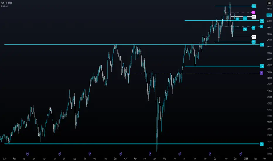
Kripto Fema ind/ This Pine Script™ code is subject to the terms of the Mozilla Public License 2.0 at mozilla.org
// © Femayakup
//@version=5
indicator(title = "Kripto Fema ind", shorttitle="Kripto Fema ind", overlay=true, format=format.price, precision=2,max_lines_count = 500, max_labels_count = 500, max_bars_back=500)
showEma200 = input(true, title="EMA 200")
showPmax = input(true, title="Pmax")
showLinreg = input(true, title="Linreg")
showMavilim = input(true, title="Mavilim")
showNadaray = input(true, title="Nadaraya Watson")
ma(source, length, type) =>
switch type
"SMA" => ta.sma(source, length)
"EMA" => ta.ema(source, length)
"SMMA (RMA)" => ta.rma(source, length)
"WMA" => ta.wma(source, length)
"VWMA" => ta.vwma(source, length)
//Ema200
timeFrame = input.timeframe(defval = '240',title= 'EMA200 TimeFrame',group = 'EMA200 Settings')
len200 = input.int(200, minval=1, title="Length",group = 'EMA200 Settings')
src200 = input(close, title="Source",group = 'EMA200 Settings')
offset200 = input.int(title="Offset", defval=0, minval=-500, maxval=500,group = 'EMA200 Settings')
out200 = ta.ema(src200, len200)
higherTimeFrame = request.security(syminfo.tickerid,timeFrame,out200 ,barmerge.gaps_on,barmerge.lookahead_on)
ema200Plot = showEma200 ? higherTimeFrame : na
plot(ema200Plot, title="EMA200", offset=offset200)
//Linreq
group1 = "Linreg Settings"
lengthInput = input.int(100, title="Length", minval = 1, maxval = 5000,group = group1)
sourceInput = input.source(close, title="Source")
useUpperDevInput = input.bool(true, title="Upper Deviation", inline = "Upper Deviation", group = group1)
upperMultInput = input.float(2.0, title="", inline = "Upper Deviation", group = group1)
useLowerDevInput = input.bool(true, title="Lower Deviation", inline = "Lower Deviation", group = group1)
lowerMultInput = input.float(2.0, title="", inline = "Lower Deviation", group = group1)
group2 = "Linreg Display Settings"
showPearsonInput = input.bool(true, "Show Pearson's R", group = group2)
extendLeftInput = input.bool(false, "Extend Lines Left", group = group2)
extendRightInput = input.bool(true, "Extend Lines Right", group = group2)
extendStyle = switch
extendLeftInput and extendRightInput => extend.both
extendLeftInput => extend.left
extendRightInput => extend.right
=> extend.none
group3 = "Linreg Color Settings"
colorUpper = input.color(color.new(color.blue, 85), "Linreg Renk", inline = group3, group = group3)
colorLower = input.color(color.new(color.red, 85), "", inline = group3, group = group3)
calcSlope(source, length) =>
max_bars_back(source, 5000)
if not barstate.islast or length <= 1
else
sumX = 0.0
sumY = 0.0
sumXSqr = 0.0
sumXY = 0.0
for i = 0 to length - 1 by 1
val = source
per = i + 1.0
sumX += per
sumY += val
sumXSqr += per * per
sumXY += val * per
slope = (length * sumXY - sumX * sumY) / (length * sumXSqr - sumX * sumX)
average = sumY / length
intercept = average - slope * sumX / length + slope
= calcSlope(sourceInput, lengthInput)
startPrice = i + s * (lengthInput - 1)
endPrice = i
var line baseLine = na
if na(baseLine) and not na(startPrice) and showLinreg
baseLine := line.new(bar_index - lengthInput + 1, startPrice, bar_index, endPrice, width=1, extend=extendStyle, color=color.new(colorLower, 0))
else
line.set_xy1(baseLine, bar_index - lengthInput + 1, startPrice)
line.set_xy2(baseLine, bar_index, endPrice)
na
calcDev(source, length, slope, average, intercept) =>
upDev = 0.0
dnDev = 0.0
stdDevAcc = 0.0
dsxx = 0.0
dsyy = 0.0
dsxy = 0.0
periods = length - 1
daY = intercept + slope * periods / 2
val = intercept
for j = 0 to periods by 1
price = high - val
if price > upDev
upDev := price
price := val - low
if price > dnDev
dnDev := price
price := source
dxt = price - average
dyt = val - daY
price -= val
stdDevAcc += price * price
dsxx += dxt * dxt
dsyy += dyt * dyt
dsxy += dxt * dyt
val += slope
stdDev = math.sqrt(stdDevAcc / (periods == 0 ? 1 : periods))
pearsonR = dsxx == 0 or dsyy == 0 ? 0 : dsxy / math.sqrt(dsxx * dsyy)
= calcDev(sourceInput, lengthInput, s, a, i)
upperStartPrice = startPrice + (useUpperDevInput ? upperMultInput * stdDev : upDev)
upperEndPrice = endPrice + (useUpperDevInput ? upperMultInput * stdDev : upDev)
var line upper = na
lowerStartPrice = startPrice + (useLowerDevInput ? -lowerMultInput * stdDev : -dnDev)
lowerEndPrice = endPrice + (useLowerDevInput ? -lowerMultInput * stdDev : -dnDev)
var line lower = na
if na(upper) and not na(upperStartPrice) and showLinreg
upper := line.new(bar_index - lengthInput + 1, upperStartPrice, bar_index, upperEndPrice, width=1, extend=extendStyle, color=color.new(colorUpper, 0))
else
line.set_xy1(upper, bar_index - lengthInput + 1, upperStartPrice)
line.set_xy2(upper, bar_index, upperEndPrice)
na
if na(lower) and not na(lowerStartPrice) and showLinreg
lower := line.new(bar_index - lengthInput + 1, lowerStartPrice, bar_index, lowerEndPrice, width=1, extend=extendStyle, color=color.new(colorUpper, 0))
else
line.set_xy1(lower, bar_index - lengthInput + 1, lowerStartPrice)
line.set_xy2(lower, bar_index, lowerEndPrice)
na
showLinregPlotUpper = showLinreg ? upper : na
showLinregPlotLower = showLinreg ? lower : na
showLinregPlotBaseLine = showLinreg ? baseLine : na
linefill.new(showLinregPlotUpper, showLinregPlotBaseLine, color = colorUpper)
linefill.new(showLinregPlotBaseLine, showLinregPlotLower, color = colorLower)
// Pearson's R
var label r = na
label.delete(r )
if showPearsonInput and not na(pearsonR) and showLinreg
r := label.new(bar_index - lengthInput + 1, lowerStartPrice, str.tostring(pearsonR, "#.################"), color = color.new(color.white, 100), textcolor=color.new(colorUpper, 0), size=size.normal, style=label.style_label_up)
//Mavilim
group4 = "Mavilim Settings"
mavilimold = input(false, title="Show Previous Version of MavilimW?",group=group4)
fmal=input(3,"First Moving Average length",group = group4)
smal=input(5,"Second Moving Average length",group = group4)
tmal=fmal+smal
Fmal=smal+tmal
Ftmal=tmal+Fmal
Smal=Fmal+Ftmal
M1= ta.wma(close, fmal)
M2= ta.wma(M1, smal)
M3= ta.wma(M2, tmal)
M4= ta.wma(M3, Fmal)
M5= ta.wma(M4, Ftmal)
MAVW= ta.wma(M5, Smal)
col1= MAVW>MAVW
col3= MAVWpmaxsrc ? pmaxsrc-pmaxsrc : 0
vdd1=pmaxsrc
ma = 0.0
if mav == "SMA"
ma := ta.sma(pmaxsrc, length)
ma
if mav == "EMA"
ma := ta.ema(pmaxsrc, length)
ma
if mav == "WMA"
ma := ta.wma(pmaxsrc, length)
ma
if mav == "TMA"
ma := ta.sma(ta.sma(pmaxsrc, math.ceil(length / 2)), math.floor(length / 2) + 1)
ma
if mav == "VAR"
ma := VAR
ma
if mav == "WWMA"
ma := WWMA
ma
if mav == "ZLEMA"
ma := ZLEMA
ma
if mav == "TSF"
ma := TSF
ma
ma
MAvg=getMA(pmaxsrc, length)
longStop = Normalize ? MAvg - Multiplier*atr/close : MAvg - Multiplier*atr
longStopPrev = nz(longStop , longStop)
longStop := MAvg > longStopPrev ? math.max(longStop, longStopPrev) : longStop
shortStop = Normalize ? MAvg + Multiplier*atr/close : MAvg + Multiplier*atr
shortStopPrev = nz(shortStop , shortStop)
shortStop := MAvg < shortStopPrev ? math.min(shortStop, shortStopPrev) : shortStop
dir = 1
dir := nz(dir , dir)
dir := dir == -1 and MAvg > shortStopPrev ? 1 : dir == 1 and MAvg < longStopPrev ? -1 : dir
PMax = dir==1 ? longStop: shortStop
plot(showsupport ? MAvg : na, color=#fbff04, linewidth=2, title="EMA9")
pALL=plot(PMax, color=color.new(color.red, transp = 0), linewidth=2, title="PMax")
alertcondition(ta.cross(MAvg, PMax), title="Cross Alert", message="PMax - Moving Avg Crossing!")
alertcondition(ta.crossover(MAvg, PMax), title="Crossover Alarm", message="Moving Avg BUY SIGNAL!")
alertcondition(ta.crossunder(MAvg, PMax), title="Crossunder Alarm", message="Moving Avg SELL SIGNAL!")
alertcondition(ta.cross(pmaxsrc, PMax), title="Price Cross Alert", message="PMax - Price Crossing!")
alertcondition(ta.crossover(pmaxsrc, PMax), title="Price Crossover Alarm", message="PRICE OVER PMax - BUY SIGNAL!")
alertcondition(ta.crossunder(pmaxsrc, PMax), title="Price Crossunder Alarm", message="PRICE UNDER PMax - SELL SIGNAL!")
buySignalk = ta.crossover(MAvg, PMax)
plotshape(buySignalk and showsignalsk ? PMax*0.995 : na, title="Buy", text="Buy", location=location.absolute, style=shape.labelup, size=size.tiny, color=color.new(color.green, transp = 0), textcolor=color.white)
sellSignallk = ta.crossunder(MAvg, PMax)
plotshape(sellSignallk and showsignalsk ? PMax*1.005 : na, title="Sell", text="Sell", location=location.absolute, style=shape.labeldown, size=size.tiny, color=color.new(color.red, transp = 0), textcolor=color.white)
// buySignalc = ta.crossover(pmaxsrc, PMax)
// plotshape(buySignalc and showsignalsc ? PMax*0.995 : na, title="Buy", text="Buy", location=location.absolute, style=shape.labelup, size=size.tiny, color=#0F18BF, textcolor=color.white)
// sellSignallc = ta.crossunder(pmaxsrc, PMax)
// plotshape(sellSignallc and showsignalsc ? PMax*1.005 : na, title="Sell", text="Sell", location=location.absolute, style=shape.labeldown, size=size.tiny, color=#0F18BF, textcolor=color.white)
// mPlot = plot(ohlc4, title="", style=plot.style_circles, linewidth=0,display=display.none)
longFillColor = highlighting ? (MAvg>PMax ? color.new(color.green, transp = 90) : na) : na
shortFillColor = highlighting ? (MAvg math.exp(-(math.pow(x, 2)/(h * h * 2)))
//-----------------------------------------------------------------------------}
//Append lines
//-----------------------------------------------------------------------------{
n = bar_index
var ln = array.new_line(0)
if barstate.isfirst and repaint
for i = 0 to 499
array.push(ln,line.new(na,na,na,na))
//-----------------------------------------------------------------------------}
//End point method
//-----------------------------------------------------------------------------{
var coefs = array.new_float(0)
var den = 0.
if barstate.isfirst and not repaint
for i = 0 to 499
w = gauss(i, h)
coefs.push(w)
den := coefs.sum()
out = 0.
if not repaint
for i = 0 to 499
out += src * coefs.get(i)
out /= den
mae = ta.sma(math.abs(src - out), 499) * mult
upperN = out + mae
lowerN = out - mae
//-----------------------------------------------------------------------------}
//Compute and display NWE
//-----------------------------------------------------------------------------{
float y2 = na
float y1 = na
nwe = array.new(0)
if barstate.islast and repaint
sae = 0.
//Compute and set NWE point
for i = 0 to math.min(499,n - 1)
sum = 0.
sumw = 0.
//Compute weighted mean
for j = 0 to math.min(499,n - 1)
w = gauss(i - j, h)
sum += src * w
sumw += w
y2 := sum / sumw
sae += math.abs(src - y2)
nwe.push(y2)
sae := sae / math.min(499,n - 1) * mult
for i = 0 to math.min(499,n - 1)
if i%2 and showNadaray
line.new(n-i+1, y1 + sae, n-i, nwe.get(i) + sae, color = upCss)
line.new(n-i+1, y1 - sae, n-i, nwe.get(i) - sae, color = dnCss)
if src > nwe.get(i) + sae and src < nwe.get(i) + sae and showNadaray
label.new(n-i, src , '▼', color = color(na), style = label.style_label_down, textcolor = dnCss, textalign = text.align_center)
if src < nwe.get(i) - sae and src > nwe.get(i) - sae and showNadaray
label.new(n-i, src , '▲', color = color(na), style = label.style_label_up, textcolor = upCss, textalign = text.align_center)
y1 := nwe.get(i)
//-----------------------------------------------------------------------------}
//Dashboard
//-----------------------------------------------------------------------------{
var tb = table.new(position.top_right, 1, 1
, bgcolor = #1e222d
, border_color = #373a46
, border_width = 1
, frame_color = #373a46
, frame_width = 1)
if repaint
tb.cell(0, 0, 'Repainting Mode Enabled', text_color = color.white, text_size = size.small)
//-----------------------------------------------------------------------------}
//Plot
//-----------------------------------------------------------------------------}
// plot(repaint ? na : out + mae, 'Upper', upCss)
// plot(repaint ? na : out - mae, 'Lower', dnCss)
//Crossing Arrows
// plotshape(ta.crossunder(close, out - mae) ? low : na, "Crossunder", shape.labelup, location.absolute, color(na), 0 , text = '▲', textcolor = upCss, size = size.tiny)
// plotshape(ta.crossover(close, out + mae) ? high : na, "Crossover", shape.labeldown, location.absolute, color(na), 0 , text = '▼', textcolor = dnCss, size = size.tiny)
//-----------------------------------------------------------------------------}
//////////////////////////////////////////////////////////////////////////////////
enableD = input (true, "DIVERGANCE ON/OFF" , group="INDICATORS ON/OFF")
//DIVERGANCE
prd1 = input.int (defval=5 , title='PIVOT PERIOD' , minval=1, maxval=50 , group="DIVERGANCE")
source = input.string(defval='HIGH/LOW' , title='SOURCE FOR PIVOT POINTS' , options= , group="DIVERGANCE")
searchdiv = input.string(defval='REGULAR/HIDDEN', title='DIVERGANCE TYPE' , options= , group="DIVERGANCE")
showindis = input.string(defval='FULL' , title='SHOW INDICATORS NAME' , options= , group="DIVERGANCE")
showlimit = input.int(1 , title='MINIMUM NUMBER OF DIVERGANCES', minval=1, maxval=11 , group="DIVERGANCE")
maxpp = input.int (defval=20 , title='MAXIMUM PIVOT POINTS TO CHECK', minval=1, maxval=20 , group="DIVERGANCE")
maxbars = input.int (defval=200 , title='MAXIMUM BARS TO CHECK' , minval=30, maxval=200 , group="DIVERGANCE")
showlast = input (defval=false , title='SHOW ONLY LAST DIVERGANCE' , group="DIVERGANCE")
dontconfirm = input (defval=false , title="DON'T WAIT FOR CONFORMATION" , group="DIVERGANCE")
showlines = input (defval=false , title='SHOW DIVERGANCE LINES' , group="DIVERGANCE")
showpivot = input (defval=false , title='SHOW PIVOT POINTS' , group="DIVERGANCE")
calcmacd = input (defval=true , title='MACD' , group="DIVERGANCE")
calcmacda = input (defval=true , title='MACD HISTOGRAM' , group="DIVERGANCE")
calcrsi = input (defval=true , title='RSI' , group="DIVERGANCE")
calcstoc = input (defval=true , title='STOCHASTIC' , group="DIVERGANCE")
calccci = input (defval=true , title='CCI' , group="DIVERGANCE")
calcmom = input (defval=true , title='MOMENTUM' , group="DIVERGANCE")
calcobv = input (defval=true , title='OBV' , group="DIVERGANCE")
calcvwmacd = input (true , title='VWMACD' , group="DIVERGANCE")
calccmf = input (true , title='CHAIKIN MONEY FLOW' , group="DIVERGANCE")
calcmfi = input (true , title='MONEY FLOW INDEX' , group="DIVERGANCE")
calcext = input (false , title='CHECK EXTERNAL INDICATOR' , group="DIVERGANCE")
externalindi = input (defval=close , title='EXTERNAL INDICATOR' , group="DIVERGANCE")
pos_reg_div_col = input (defval=#ffffff , title='POSITIVE REGULAR DIVERGANCE' , group="DIVERGANCE")
neg_reg_div_col = input (defval=#00def6 , title='NEGATIVE REGULAR DIVERGANCE' , group="DIVERGANCE")
pos_hid_div_col = input (defval=#00ff0a , title='POSITIVE HIDDEN DIVERGANCE' , group="DIVERGANCE")
neg_hid_div_col = input (defval=#ff0015 , title='NEGATIVE HIDDEN DIVERGANCE' , group="DIVERGANCE")
reg_div_l_style_ = input.string(defval='SOLID' , title='REGULAR DIVERGANCE LINESTYLE' , options= , group="DIVERGANCE")
hid_div_l_style_ = input.string(defval='SOLID' , title='HIDDEN DIVERGANCE LINESTYLE' , options= , group="DIVERGANCE")
reg_div_l_width = input.int (defval=2 , title='REGULAR DIVERGANCE LINEWIDTH' , minval=1, maxval=5 , group="DIVERGANCE")
hid_div_l_width = input.int (defval=2 , title='HIDDEN DIVERGANCE LINEWIDTH' , minval=1, maxval=5 , group="DIVERGANCE")
showmas = input.bool (defval=false , title='SHOW MOVING AVERAGES (50 & 200)', inline='MA' , group="DIVERGANCE")
cma1col = input.color (defval=#ffffff , title='' , inline='MA' , group="DIVERGANCE")
cma2col = input.color (defval=#00def6 , title='' , inline='MA' , group="DIVERGANCE")
//PLOTS
plot(showmas ? ta.sma(close, 50) : na, color=showmas ? cma1col : na)
plot(showmas ? ta.sma(close, 200) : na, color=showmas ? cma2col : na)
var reg_div_l_style = reg_div_l_style_ == 'SOLID' ? line.style_solid : reg_div_l_style_ == 'DASHED' ? line.style_dashed : line.style_dotted
var hid_div_l_style = hid_div_l_style_ == 'SOLID' ? line.style_solid : hid_div_l_style_ == 'DASHED' ? line.style_dashed : line.style_dotted
rsi = ta.rsi(close, 14)
= ta.macd(close, 12, 26, 9)
moment = ta.mom(close, 10)
cci = ta.cci(close, 10)
Obv = ta.obv
stk = ta.sma(ta.stoch(close, high, low, 14), 3)
maFast = ta.vwma(close, 12)
maSlow = ta.vwma(close, 26)
vwmacd = maFast - maSlow
Cmfm = (close - low - (high - close)) / (high - low)
Cmfv = Cmfm * volume
cmf = ta.sma(Cmfv, 21) / ta.sma(volume, 21)
Mfi = ta.mfi(close, 14)
var indicators_name = array.new_string(11)
var div_colors = array.new_color(4)
if barstate.isfirst and enableD
array.set(indicators_name, 0, showindis == "DON'T SHOW" ? '' : '')
array.set(indicators_name, 1, showindis == "DON'T SHOW" ? '' : '')
array.set(indicators_name, 2, showindis == "DON'T SHOW" ? '' : '')
array.set(indicators_name, 3, showindis == "DON'T SHOW" ? '' : '')
array.set(indicators_name, 4, showindis == "DON'T SHOW" ? '' : '')
array.set(indicators_name, 5, showindis == "DON'T SHOW" ? '' : '')
array.set(indicators_name, 6, showindis == "DON'T SHOW" ? '' : '')
array.set(indicators_name, 7, showindis == "DON'T SHOW" ? '' : '')
array.set(indicators_name, 8, showindis == "DON'T SHOW" ? '' : '')
array.set(indicators_name, 9, showindis == "DON'T SHOW" ? '' : '')
array.set(indicators_name, 10, showindis == "DON'T SHOW" ? '' : '')
array.set(div_colors, 0, pos_reg_div_col)
array.set(div_colors, 1, neg_reg_div_col)
array.set(div_colors, 2, pos_hid_div_col)
array.set(div_colors, 3, neg_hid_div_col)
float ph1 = ta.pivothigh(source == 'CLOSE' ? close : high, prd1, prd1)
float pl1 = ta.pivotlow(source == 'CLOSE' ? close : low, prd1, prd1)
plotshape(ph1 and showpivot, text='H', style=shape.labeldown, color=color.new(color.white, 100), textcolor=#00def6, location=location.abovebar, offset=-prd1)
plotshape(pl1 and showpivot, text='L', style=shape.labelup, color=color.new(color.white, 100), textcolor=#ffffff, location=location.belowbar, offset=-prd1)
var int maxarraysize = 20
var ph_positions = array.new_int(maxarraysize, 0)
var pl_positions = array.new_int(maxarraysize, 0)
var ph_vals = array.new_float(maxarraysize, 0.)
var pl_vals = array.new_float(maxarraysize, 0.)
if ph1
array.unshift(ph_positions, bar_index)
array.unshift(ph_vals, ph1)
if array.size(ph_positions) > maxarraysize
array.pop(ph_positions)
array.pop(ph_vals)
if pl1
array.unshift(pl_positions, bar_index)
array.unshift(pl_vals, pl1)
if array.size(pl_positions) > maxarraysize
array.pop(pl_positions)
array.pop(pl_vals)
positive_regular_positive_hidden_divergence(src, cond) =>
divlen = 0
prsc = source == 'CLOSE' ? close : low
if dontconfirm or src > src or close > close
startpoint = dontconfirm ? 0 : 1
for x = 0 to maxpp - 1 by 1
len = bar_index - array.get(pl_positions, x) + prd1
if array.get(pl_positions, x) == 0 or len > maxbars
break
if len > 5 and (cond == 1 and src > src and prsc < nz(array.get(pl_vals, x)) or cond == 2 and src < src and prsc > nz(array.get(pl_vals, x)))
slope1 = (src - src ) / (len - startpoint)
virtual_line1 = src - slope1
slope2 = (close - close ) / (len - startpoint)
virtual_line2 = close - slope2
arrived = true
for y = 1 + startpoint to len - 1 by 1
if src < virtual_line1 or nz(close ) < virtual_line2
arrived := false
break
virtual_line1 -= slope1
virtual_line2 -= slope2
virtual_line2
if arrived
divlen := len
break
divlen
negative_regular_negative_hidden_divergence(src, cond) =>
divlen = 0
prsc = source == 'CLOSE' ? close : high
if dontconfirm or src < src or close < close
startpoint = dontconfirm ? 0 : 1
for x = 0 to maxpp - 1 by 1
len = bar_index - array.get(ph_positions, x) + prd1
if array.get(ph_positions, x) == 0 or len > maxbars
break
if len > 5 and (cond == 1 and src < src and prsc > nz(array.get(ph_vals, x)) or cond == 2 and src > src and prsc < nz(array.get(ph_vals, x)))
slope1 = (src - src ) / (len - startpoint)
virtual_line1 = src - slope1
slope2 = (close - nz(close )) / (len - startpoint)
virtual_line2 = close - slope2
arrived = true
for y = 1 + startpoint to len - 1 by 1
if src > virtual_line1 or nz(close ) > virtual_line2
arrived := false
break
virtual_line1 -= slope1
virtual_line2 -= slope2
virtual_line2
if arrived
divlen := len
break
divlen
//CALCULATIONS
calculate_divs(cond, indicator_1) =>
divs = array.new_int(4, 0)
array.set(divs, 0, cond and (searchdiv == 'REGULAR' or searchdiv == 'REGULAR/HIDDEN') ? positive_regular_positive_hidden_divergence(indicator_1, 1) : 0)
array.set(divs, 1, cond and (searchdiv == 'REGULAR' or searchdiv == 'REGULAR/HIDDEN') ? negative_regular_negative_hidden_divergence(indicator_1, 1) : 0)
array.set(divs, 2, cond and (searchdiv == 'HIDDEN' or searchdiv == 'REGULAR/HIDDEN') ? positive_regular_positive_hidden_divergence(indicator_1, 2) : 0)
array.set(divs, 3, cond and (searchdiv == 'HIDDEN' or searchdiv == 'REGULAR/HIDDEN') ? negative_regular_negative_hidden_divergence(indicator_1, 2) : 0)
divs
var all_divergences = array.new_int(44)
array_set_divs(div_pointer, index) =>
for x = 0 to 3 by 1
array.set(all_divergences, index * 4 + x, array.get(div_pointer, x))
array_set_divs(calculate_divs(calcmacd , macd) , 0)
array_set_divs(calculate_divs(calcmacda , deltamacd) , 1)
array_set_divs(calculate_divs(calcrsi , rsi) , 2)
array_set_divs(calculate_divs(calcstoc , stk) , 3)
array_set_divs(calculate_divs(calccci , cci) , 4)
array_set_divs(calculate_divs(calcmom , moment) , 5)
array_set_divs(calculate_divs(calcobv , Obv) , 6)
array_set_divs(calculate_divs(calcvwmacd, vwmacd) , 7)
array_set_divs(calculate_divs(calccmf , cmf) , 8)
array_set_divs(calculate_divs(calcmfi , Mfi) , 9)
array_set_divs(calculate_divs(calcext , externalindi), 10)
total_div = 0
for x = 0 to array.size(all_divergences) - 1 by 1
total_div += math.round(math.sign(array.get(all_divergences, x)))
total_div
if total_div < showlimit
array.fill(all_divergences, 0)
var pos_div_lines = array.new_line(0)
var neg_div_lines = array.new_line(0)
var pos_div_labels = array.new_label(0)
var neg_div_labels = array.new_label(0)
delete_old_pos_div_lines() =>
if array.size(pos_div_lines) > 0
for j = 0 to array.size(pos_div_lines) - 1 by 1
line.delete(array.get(pos_div_lines, j))
array.clear(pos_div_lines)
delete_old_neg_div_lines() =>
if array.size(neg_div_lines) > 0
for j = 0 to array.size(neg_div_lines) - 1 by 1
line.delete(array.get(neg_div_lines, j))
array.clear(neg_div_lines)
delete_old_pos_div_labels() =>
if array.size(pos_div_labels) > 0
for j = 0 to array.size(pos_div_labels) - 1 by 1
label.delete(array.get(pos_div_labels, j))
array.clear(pos_div_labels)
delete_old_neg_div_labels() =>
if array.size(neg_div_labels) > 0
for j = 0 to array.size(neg_div_labels) - 1 by 1
label.delete(array.get(neg_div_labels, j))
array.clear(neg_div_labels)
delete_last_pos_div_lines_label(n) =>
if n > 0 and array.size(pos_div_lines) >= n
asz = array.size(pos_div_lines)
for j = 1 to n by 1
line.delete(array.get(pos_div_lines, asz - j))
array.pop(pos_div_lines)
if array.size(pos_div_labels) > 0
label.delete(array.get(pos_div_labels, array.size(pos_div_labels) - 1))
array.pop(pos_div_labels)
delete_last_neg_div_lines_label(n) =>
if n > 0 and array.size(neg_div_lines) >= n
asz = array.size(neg_div_lines)
for j = 1 to n by 1
line.delete(array.get(neg_div_lines, asz - j))
array.pop(neg_div_lines)
if array.size(neg_div_labels) > 0
label.delete(array.get(neg_div_labels, array.size(neg_div_labels) - 1))
array.pop(neg_div_labels)
pos_reg_div_detected = false
neg_reg_div_detected = false
pos_hid_div_detected = false
neg_hid_div_detected = false
var last_pos_div_lines = 0
var last_neg_div_lines = 0
var remove_last_pos_divs = false
var remove_last_neg_divs = false
if pl1
remove_last_pos_divs := false
last_pos_div_lines := 0
last_pos_div_lines
if ph1
remove_last_neg_divs := false
last_neg_div_lines := 0
last_neg_div_lines
divergence_text_top = ''
divergence_text_bottom = ''
distances = array.new_int(0)
dnumdiv_top = 0
dnumdiv_bottom = 0
top_label_col = color.white
bottom_label_col = color.white
old_pos_divs_can_be_removed = true
old_neg_divs_can_be_removed = true
startpoint = dontconfirm ? 0 : 1
for x = 0 to 10 by 1
div_type = -1
for y = 0 to 3 by 1
if array.get(all_divergences, x * 4 + y) > 0
div_type := y
if y % 2 == 1
dnumdiv_top += 1
top_label_col := array.get(div_colors, y)
top_label_col
if y % 2 == 0
dnumdiv_bottom += 1
bottom_label_col := array.get(div_colors, y)
bottom_label_col
if not array.includes(distances, array.get(all_divergences, x * 4 + y))
array.push(distances, array.get(all_divergences, x * 4 + y))
new_line = showlines ? line.new(x1=bar_index - array.get(all_divergences, x * 4 + y), y1=source == 'CLOSE' ? close : y % 2 == 0 ? low : high , x2=bar_index - startpoint, y2=source == 'CLOSE' ? close : y % 2 == 0 ? low : high , color=array.get(div_colors, y), style=y < 2 ? reg_div_l_style : hid_div_l_style, width=y < 2 ? reg_div_l_width : hid_div_l_width) : na
if y % 2 == 0
if old_pos_divs_can_be_removed
old_pos_divs_can_be_removed := false
if not showlast and remove_last_pos_divs
delete_last_pos_div_lines_label(last_pos_div_lines)
last_pos_div_lines := 0
last_pos_div_lines
if showlast
delete_old_pos_div_lines()
array.push(pos_div_lines, new_line)
last_pos_div_lines += 1
remove_last_pos_divs := true
remove_last_pos_divs
if y % 2 == 1
if old_neg_divs_can_be_removed
old_neg_divs_can_be_removed := false
if not showlast and remove_last_neg_divs
delete_last_neg_div_lines_label(last_neg_div_lines)
last_neg_div_lines := 0
last_neg_div_lines
if showlast
delete_old_neg_div_lines()
array.push(neg_div_lines, new_line)
last_neg_div_lines += 1
remove_last_neg_divs := true
remove_last_neg_divs
if y == 0
pos_reg_div_detected := true
pos_reg_div_detected
if y == 1
neg_reg_div_detected := true
neg_reg_div_detected
if y == 2
pos_hid_div_detected := true
pos_hid_div_detected
if y == 3
neg_hid_div_detected := true
neg_hid_div_detected
if div_type >= 0
divergence_text_top += (div_type % 2 == 1 ? showindis != "DON'T SHOW" ? array.get(indicators_name, x) + '\n' : '' : '')
divergence_text_bottom += (div_type % 2 == 0 ? showindis != "DON'T SHOW" ? array.get(indicators_name, x) + '\n' : '' : '')
divergence_text_bottom
if showindis != "DON'T SHOW"
if dnumdiv_top > 0
divergence_text_top += str.tostring(dnumdiv_top)
divergence_text_top
if dnumdiv_bottom > 0
divergence_text_bottom += str.tostring(dnumdiv_bottom)
divergence_text_bottom
if divergence_text_top != ''
if showlast
delete_old_neg_div_labels()
array.push(neg_div_labels, label.new(x=bar_index, y=math.max(high, high ), color=top_label_col, style=label.style_diamond, size = size.auto))
if divergence_text_bottom != ''
if showlast
delete_old_pos_div_labels()
array.push(pos_div_labels, label.new(x=bar_index, y=math.min(low, low ), color=bottom_label_col, style=label.style_diamond, size = size.auto))
// POSITION AND SIZE
PosTable = input.string(defval="Bottom Right", title="Position", options= , group="Table Location & Size", inline="1")
SizTable = input.string(defval="Auto", title="Size", options= , group="Table Location & Size", inline="1")
Pos1Table = PosTable == "Top Right" ? position.top_right : PosTable == "Middle Right" ? position.middle_right : PosTable == "Bottom Right" ? position.bottom_right : PosTable == "Top Center" ? position.top_center : PosTable == "Middle Center" ? position.middle_center : PosTable == "Bottom Center" ? position.bottom_center : PosTable == "Top Left" ? position.top_left : PosTable == "Middle Left" ? position.middle_left : position.bottom_left
Siz1Table = SizTable == "Auto" ? size.auto : SizTable == "Huge" ? size.huge : SizTable == "Large" ? size.large : SizTable == "Normal" ? size.normal : SizTable == "Small" ? size.small : size.tiny
tbl = table.new(Pos1Table, 21, 16, border_width = 1, border_color = color.gray, frame_color = color.gray, frame_width = 1)
// Kullanıcı tarafından belirlenecek yeşil ve kırmızı zaman dilimi sayısı
greenThreshold = input.int(5, minval=1, maxval=10, title="Yeşil Zaman Dilimi Sayısı", group="Alarm Ayarları")
redThreshold = input.int(5, minval=1, maxval=10, title="Kırmızı Zaman Dilimi Sayısı", group="Alarm Ayarları")
// TIMEFRAMES OPTIONS
box01 = input.bool(true, "TF ", inline = "01", group="Select Timeframe")
tf01 = input.timeframe("1", "", inline = "01", group="Select Timeframe")
box02 = input.bool(false, "TF ", inline = "02", group="Select Timeframe")
tf02 = input.timeframe("3", "", inline = "02", group="Select Timeframe")
box03 = input.bool(true, "TF ", inline = "03", group="Select Timeframe")
tf03 = input.timeframe("5", "", inline = "03", group="Select Timeframe")
box04 = input.bool(true, "TF ", inline = "04", group="Select Timeframe")
tf04 = input.timeframe("15", "", inline = "04", group="Select Timeframe")
box05 = input.bool(false, "TF ", inline = "05", group="Select Timeframe")
tf05 = input.timeframe("30", "", inline = "05", group="Select Timeframe")
box06 = input.bool(true, "TF ", inline = "01", group="Select Timeframe")
tf06 = input.timeframe("60", "", inline = "01", group="Select Timeframe")
box07 = input.bool(false, "TF ", inline = "02", group="Select Timeframe")
tf07 = input.timeframe("120", "", inline = "02", group="Select Timeframe")
box08 = input.bool(false, "TF ", inline = "03", group="Select Timeframe")
tf08 = input.timeframe("180", "", inline = "03", group="Select Timeframe")
box09 = input.bool(true, "TF ", inline = "04", group="Select Timeframe")
tf09 = input.timeframe("240", "", inline = "04", group="Select Timeframe")
box10 = input.bool(false, "TF ", inline = "05", group="Select Timeframe")
tf10 = input.timeframe("D", "", inline = "05", group="Select Timeframe")
// indicator('Tillson FEMA', overlay=true)
length1 = input(1, 'FEMA Length')
a1 = input(0.7, 'Volume Factor')
e1 = ta.ema((high + low + 2 * close) / 4, length1)
e2 = ta.ema(e1, length1)
e3 = ta.ema(e2, length1)
e4 = ta.ema(e3, length1)
e5 = ta.ema(e4, length1)
e6 = ta.ema(e5, length1)
c1 = -a1 * a1 * a1
c2 = 3 * a1 * a1 + 3 * a1 * a1 * a1
c3 = -6 * a1 * a1 - 3 * a1 - 3 * a1 * a1 * a1
c4 = 1 + 3 * a1 + a1 * a1 * a1 + 3 * a1 * a1
FEMA = c1 * e6 + c2 * e5 + c3 * e4 + c4 * e3
tablocol1 = FEMA > FEMA
tablocol3 = FEMA < FEMA
color_1 = col1 ? color.rgb(149, 219, 35): col3 ? color.rgb(238, 11, 11) : color.yellow
plot(FEMA, color=color_1, linewidth=3, title='FEMA')
tilson1 = FEMA
tilson1a =FEMA
// DEFINITION OF VALUES
symbol = ticker.modify(syminfo.tickerid, syminfo.session)
tfArr = array.new(na)
tilson1Arr = array.new(na)
tilson1aArr = array.new(na)
// DEFINITIONS OF RSI & CCI FUNCTIONS APPENDED IN THE TIMEFRAME OPTIONS
cciNcciFun(tf, flg) =>
= request.security(symbol, tf, )
if flg and (barstate.isrealtime ? true : timeframe.in_seconds(timeframe.period) <= timeframe.in_seconds(tf))
array.push(tfArr, na(tf) ? timeframe.period : tf)
array.push(tilson1Arr, tilson_)
array.push(tilson1aArr, tilson1a_)
cciNcciFun(tf01, box01), cciNcciFun(tf02, box02), cciNcciFun(tf03, box03), cciNcciFun(tf04, box04),
cciNcciFun(tf05, box05), cciNcciFun(tf06, box06), cciNcciFun(tf07, box07), cciNcciFun(tf08, box08),
cciNcciFun(tf09, box09), cciNcciFun(tf10, box10)
// TABLE AND CELLS CONFIG
// Post Timeframe in format
tfTxt(x)=>
out = x
if not str.contains(x, "S") and not str.contains(x, "M") and
not str.contains(x, "W") and not str.contains(x, "D")
if str.tonumber(x)%60 == 0
out := str.tostring(str.tonumber(x)/60)+"H"
else
out := x + "m"
out
if barstate.islast
table.clear(tbl, 0, 0, 20, 15)
// TITLES
table.cell(tbl, 0, 0, "⏱", text_color=color.white, text_size=Siz1Table, bgcolor=#000000)
table.cell(tbl, 1, 0, "FEMA("+str.tostring(length1)+")", text_color=#FFFFFF, text_size=Siz1Table, bgcolor=#000000)
j = 1
greenCounter = 0 // Yeşil zaman dilimlerini saymak için bir sayaç
redCounter = 0
if array.size(tilson1Arr) > 0
for i = 0 to array.size(tilson1Arr) - 1
if not na(array.get(tilson1Arr, i))
//config values in the cells
TF_VALUE = array.get(tfArr,i)
tilson1VALUE = array.get(tilson1Arr, i)
tilson1aVALUE = array.get(tilson1aArr, i)
SIGNAL1 = tilson1VALUE >= tilson1aVALUE ? "▲" : tilson1VALUE <= tilson1aVALUE ? "▼" : na
// Yeşil oklar ve arka planı ayarla
greenArrowColor1 = SIGNAL1 == "▲" ? color.rgb(0, 255, 0) : color.rgb(255, 0, 0)
greenBgColor1 = SIGNAL1 == "▲" ? color.rgb(25, 70, 22) : color.rgb(93, 22, 22)
allGreen = tilson1VALUE >= tilson1aVALUE
allRed = tilson1VALUE <= tilson1aVALUE
// Determine background color for time text
timeBgColor = allGreen ? #194616 : (allRed ? #5D1616 : #000000)
txtColor = allGreen ? #00FF00 : (allRed ? #FF4500 : color.white)
if allGreen
greenCounter := greenCounter + 1
redCounter := 0
else if allRed
redCounter := redCounter + 1
greenCounter := 0
else
redCounter := 0
greenCounter := 0
// Dinamik pair değerini oluşturma
pair = "USDT_" + syminfo.basecurrency + "USDT"
// Bot ID için kullanıcı girişi
bot_id = input.int(12387976, title="Bot ID", minval=0,group ='3Comas Message', inline = '1') // Varsayılan değeri 12387976 olan bir tamsayı girişi alır
// E-posta tokenı için kullanıcı girişi
email_token = input("cd4111d4-549a-4759-a082-e8f45c91fa47", title="Email Token",group ='3Comas Message', inline = '1')
// USER INPUT FOR DELAY
delay_seconds = input.int(0, title="Delay Seconds", minval=0, maxval=86400,group ='3Comas Message', inline = '1')
// Dinamik mesajın oluşturulması
message = '{ "message_type": "bot", "bot_id": ' + str.tostring(bot_id) + ', "email_token": "' + email_token + '", "delay_seconds": ' + str.tostring(delay_seconds) + ', "pair": "' + pair + '"}'
// Kullanıcının belirlediği yeşil veya kırmızı zaman dilimi sayısına ulaşıldığında alarmı tetikle
if greenCounter >= greenThreshold
alert(message, alert.freq_once_per_bar_close)
// if redCounter >= redThreshold
// alert(message, alert.freq_once_per_bar_close)
// Kullanıcının belirlediği yeşil veya kırmızı zaman dilimi sayısına ulaşıldığında alarmı tetikle
// if greenCounter >= greenThreshold
// alert("Yeşil zaman dilimi sayısı " + str.tostring(greenThreshold) + " adede ulaştı", alert.freq_once_per_bar_close)
// if redCounter >= redThreshold
// alert("Kırmızı zaman dilimi sayısı " + str.tostring(redThreshold) + " adede ulaştı", alert.freq_once_per_bar_close)
table.cell(tbl, 0, j, tfTxt(TF_VALUE), text_color=txtColor, text_halign=text.align_left, text_size=Siz1Table, bgcolor=timeBgColor)
table.cell(tbl, 1, j, str.tostring(tilson1VALUE, "#.#######")+SIGNAL1, text_color=greenArrowColor1, text_halign=text.align_right, text_size=Siz1Table, bgcolor=greenBgColor1)
j += 1
prd = input.int(defval=10, title='Pivot Period', minval=4, maxval=30, group='Setup')
ppsrc = input.string(defval='High/Low', title='Source', options= , group='Setup')
maxnumpp = input.int(defval=20, title=' Maximum Number of Pivot', minval=5, maxval=100, group='Setup')
ChannelW = input.int(defval=10, title='Maximum Channel Width %', minval=1, group='Setup')
maxnumsr = input.int(defval=5, title=' Maximum Number of S/R', minval=1, maxval=10, group='Setup')
min_strength = input.int(defval=2, title=' Minimum Strength', minval=1, maxval=10, group='Setup')
labelloc = input.int(defval=20, title='Label Location', group='Colors', tooltip='Positive numbers reference future bars, negative numbers reference histical bars')
linestyle = input.string(defval='Dashed', title='Line Style', options= , group='Colors')
linewidth = input.int(defval=2, title='Line Width', minval=1, maxval=4, group='Colors')
resistancecolor = input.color(defval=color.red, title='Resistance Color', group='Colors')
supportcolor = input.color(defval=color.lime, title='Support Color', group='Colors')
showpp = input(false, title='Show Point Points')
float src1 = ppsrc == 'High/Low' ? high : math.max(close, open)
float src2 = ppsrc == 'High/Low' ? low : math.min(close, open)
float ph = ta.pivothigh(src1, prd, prd)
float pl = ta.pivotlow(src2, prd, prd)
plotshape(ph and showpp, text='H', style=shape.labeldown, color=na, textcolor=color.new(color.red, 0), location=location.abovebar, offset=-prd)
plotshape(pl and showpp, text='L', style=shape.labelup, color=na, textcolor=color.new(color.lime, 0), location=location.belowbar, offset=-prd)
Lstyle = linestyle == 'Dashed' ? line.style_dashed : linestyle == 'Solid' ? line.style_solid : line.style_dotted
//calculate maximum S/R channel zone width
prdhighest = ta.highest(300)
prdlowest = ta.lowest(300)
cwidth = (prdhighest - prdlowest) * ChannelW / 100
var pivotvals = array.new_float(0)
if ph or pl
array.unshift(pivotvals, ph ? ph : pl)
if array.size(pivotvals) > maxnumpp // limit the array size
array.pop(pivotvals)
get_sr_vals(ind) =>
float lo = array.get(pivotvals, ind)
float hi = lo
int numpp = 0
for y = 0 to array.size(pivotvals) - 1 by 1
float cpp = array.get(pivotvals, y)
float wdth = cpp <= lo ? hi - cpp : cpp - lo
if wdth <= cwidth // fits the max channel width?
if cpp <= hi
lo := math.min(lo, cpp)
else
hi := math.max(hi, cpp)
numpp += 1
numpp
var sr_up_level = array.new_float(0)
var sr_dn_level = array.new_float(0)
sr_strength = array.new_float(0)
find_loc(strength) =>
ret = array.size(sr_strength)
for i = ret > 0 ? array.size(sr_strength) - 1 : na to 0 by 1
if strength <= array.get(sr_strength, i)
break
ret := i
ret
ret
check_sr(hi, lo, strength) =>
ret = true
for i = 0 to array.size(sr_up_level) > 0 ? array.size(sr_up_level) - 1 : na by 1
//included?
if array.get(sr_up_level, i) >= lo and array.get(sr_up_level, i) <= hi or array.get(sr_dn_level, i) >= lo and array.get(sr_dn_level, i) <= hi
if strength >= array.get(sr_strength, i)
array.remove(sr_strength, i)
array.remove(sr_up_level, i)
array.remove(sr_dn_level, i)
ret
else
ret := false
ret
break
ret
var sr_lines = array.new_line(11, na)
var sr_labels = array.new_label(11, na)
for x = 1 to 10 by 1
rate = 100 * (label.get_y(array.get(sr_labels, x)) - close) / close
label.set_text(array.get(sr_labels, x), text=str.tostring(label.get_y(array.get(sr_labels, x))) + '(' + str.tostring(rate, '#.##') + '%)')
label.set_x(array.get(sr_labels, x), x=bar_index + labelloc)
label.set_color(array.get(sr_labels, x), color=label.get_y(array.get(sr_labels, x)) >= close ? color.red : color.lime)
label.set_textcolor(array.get(sr_labels, x), textcolor=label.get_y(array.get(sr_labels, x)) >= close ? color.white : color.black)
label.set_style(array.get(sr_labels, x), style=label.get_y(array.get(sr_labels, x)) >= close ? label.style_label_down : label.style_label_up)
line.set_color(array.get(sr_lines, x), color=line.get_y1(array.get(sr_lines, x)) >= close ? resistancecolor : supportcolor)
if ph or pl
//because of new calculation, remove old S/R levels
array.clear(sr_up_level)
array.clear(sr_dn_level)
array.clear(sr_strength)
//find S/R zones
for x = 0 to array.size(pivotvals) - 1 by 1
= get_sr_vals(x)
if check_sr(hi, lo, strength)
loc = find_loc(strength)
// if strength is in first maxnumsr sr then insert it to the arrays
if loc < maxnumsr and strength >= min_strength
array.insert(sr_strength, loc, strength)
array.insert(sr_up_level, loc, hi)
array.insert(sr_dn_level, loc, lo)
// keep size of the arrays = 5
if array.size(sr_strength) > maxnumsr
array.pop(sr_strength)
array.pop(sr_up_level)
array.pop(sr_dn_level)
for x = 1 to 10 by 1
line.delete(array.get(sr_lines, x))
label.delete(array.get(sr_labels, x))
for x = 0 to array.size(sr_up_level) > 0 ? array.size(sr_up_level) - 1 : na by 1
float mid = math.round_to_mintick((array.get(sr_up_level, x) + array.get(sr_dn_level, x)) / 2)
rate = 100 * (mid - close) / close
array.set(sr_labels, x + 1, label.new(x=bar_index + labelloc, y=mid, text=str.tostring(mid) + '(' + str.tostring(rate, '#.##') + '%)', color=mid >= close ? color.red : color.lime, textcolor=mid >= close ? color.white : color.black, style=mid >= close ? label.style_label_down : label.style_label_up))
array.set(sr_lines, x + 1, line.new(x1=bar_index, y1=mid, x2=bar_index - 1, y2=mid, extend=extend.both, color=mid >= close ? resistancecolor : supportcolor, style=Lstyle, width=linewidth))
f_crossed_over() =>
ret = false
for x = 0 to array.size(sr_up_level) > 0 ? array.size(sr_up_level) - 1 : na by 1
float mid = math.round_to_mintick((array.get(sr_up_level, x) + array.get(sr_dn_level, x)) / 2)
if close <= mid and close > mid
ret := true
ret
ret
f_crossed_under() =>
ret = false
for x = 0 to array.size(sr_up_level) > 0 ? array.size(sr_up_level) - 1 : na by 1
float mid = math.round_to_mintick((array.get(sr_up_level, x) + array.get(sr_dn_level, x)) / 2)
if close >= mid and close < mid
ret := true
ret
ret
alertcondition(f_crossed_over(), title='Resistance Broken', message='Resistance Broken')
alertcondition(f_crossed_under(), title='Support Broken', message='Support Broken')

RSI Divergence (Regular + Hidden, @darshakssc)This indicator detects regular and hidden divergence between price and RSI, using confirmed swing highs and swing lows (pivots) on both series. It is designed as a visual analysis tool, not as a signal generator or trading system.
The goal is to highlight moments where price action and RSI momentum move in different directions, which some traders study as potential early warnings of trend exhaustion or trend continuation. All divergence signals are only drawn after a pivot is fully confirmed, helping to avoid repainting.
The script supports four divergence types:
Regular Bullish Divergence
Regular Bearish Divergence
Hidden Bullish Divergence
Hidden Bearish Divergence
Each type is drawn with a different color and labeled clearly on the chart.
Core Concepts Used
1. RSI (Relative Strength Index)
The script uses standard RSI, calculated on a configurable input source (default: close) and length (default: 14).
RSI is treated purely as a momentum oscillator – the script does not enforce oversold/overbought interpretations.
2. Pivots / Swings
The indicator defines swing highs and swing lows using ta.pivothigh() and ta.pivotlow():
A swing high forms when a bar’s high is higher than a specified number of bars to the left and to the right.
A swing low forms when a bar’s low is lower than a specified number of bars to the left and to the right.
The same pivot logic is applied to both price and RSI.
Because pivots require “right side” bars to form, the indicator:
Waits for the full pivot to be confirmed (no forward-looking referencing beyond the rightBars parameter).
Only then considers that pivot for divergence detection.
This helps prevent repainting of divergence signals.
How Divergence Is Detected
The script always uses the two most recent confirmed pivots for both price and RSI. It tracks:
Last two swing lows in price and RSI
Last two swing highs in price and RSI
Their pivot bar indexes and values
A basic minimum distance filter between the pivots (in bars) is also applied to reduce noise.
1. Regular Bullish Divergence
Condition:
Price makes a lower low (LL) between the last two lows
RSI makes a higher low (HL) over the same two pivot lows
The RSI difference between the two lows is greater than or equal to the user-defined minimum (Min RSI Difference)
The two low pivots are separated by at least Min Bars Between Swings
Interpretation:
Some traders view this as bearish momentum weakening while price prints a new low. The script only marks this structure; it does not assume any outcome.
On the chart:
Drawn between the previous and current price swing lows
Labeled: “Regular Bullish”
Color: Green (by default in the script)
2. Regular Bearish Divergence
Condition:
Price makes a higher high (HH) between the last two highs
RSI makes a lower high (LH) over the same two pivot highs
RSI difference exceeds Min RSI Difference
Pivots are separated by at least Min Bars Between Swings
Interpretation:
Some traders see this as bullish momentum weakening while price prints a new high. Again, the indicator simply highlights this divergence.
On the chart:
Drawn between the previous and current price swing highs
Labeled: “Regular Bearish”
Color: Red
3. Hidden Bullish Divergence
Condition:
Price makes a higher low (HL) between the last two lows
RSI makes a lower low (LL) over the same two lows
RSI difference exceeds Min RSI Difference
Pivots meet the minimum distance requirement
Interpretation:
Some traders interpret hidden bullish divergence as a potential trend continuation signal within an existing uptrend. The indicator does not classify trends; it just tags the pattern when price and RSI pivots meet the conditions.
On the chart:
Drawn between the previous and current price swing lows
Labeled: “Hidden Bullish”
Color: Teal
4. Hidden Bearish Divergence
Condition:
Price makes a lower high (LH) between the last two highs
RSI makes a higher high (HH) over those highs
RSI difference exceeds Min RSI Difference
Pivots meet the minimum distance filter
Interpretation:
Some traders associate hidden bearish divergence with potential downtrend continuation, but again, this script only visualizes the structure.
On the chart:
Drawn between the previous and current price swing highs
Labeled: “Hidden Bearish”
Color: Orange
Inputs and Settings
1. RSI Settings
RSI Source – Price source for RSI (default: close).
RSI Length – Period for RSI calculation (default: 14).
These control the responsiveness of the RSI. Shorter lengths may show more frequent divergence; longer lengths smooth the signal.
2. Swing / Pivot Settings
Left Swing Bars (leftBars)
Right Swing Bars (rightBars)
These define how strict the pivot detection is:
Higher values → fewer, more significant swings
Lower values → more swings, more signals
Because the script uses ta.pivothigh / ta.pivotlow, a pivot is only confirmed once rightBars candles have closed after the candidate bar. This is an intentional design to reduce repainting and make pivots stable.
3. Divergence Filters
Min Bars Between Swings (Min Bars Between Swings)
Requires a minimum bar distance between the two pivots used to form divergence.
Helps avoid clutter from pivots that are too close to each other.
Min RSI Difference (Min RSI Difference)
Requires a minimum absolute difference between RSI values at the two pivots.
Filters out very minor changes in RSI that may not be meaningful.
4. Visibility Toggles
Show Regular Divergence
Show Hidden Divergence
You can choose to display:
Both regular and hidden divergence, or
Only regular divergence, or
Only hidden divergence
This is useful if you prefer to focus on one type of structure.
5. Alerts
Enable Alerts
When enabled, the script exposes four alert conditions:
Regular Bullish Divergence Confirmed
Regular Bearish Divergence Confirmed
Hidden Bullish Divergence Confirmed
Hidden Bearish Divergence Confirmed
Each alert fires after the corresponding divergence has been fully confirmed based on the pivot and bar confirmation logic. The script does not issue rapid or intrabar signals; it uses confirmed historical conditions.
You can set these in the TradingView Alerts dialog by choosing this indicator and selecting the desired condition.
Visual Elements
On the main price chart, the indicator:
Draws a line between the two price pivots involved in the divergence.
Adds a small label at the latest pivot, describing the divergence type.
Colors are used to differentiate divergence categories (Green/Red/Teal/Orange).
This makes it easy to visually scan the chart for zones where price and RSI have diverged.
What to Look For (Analytical Use)
This indicator is intended as a visual helper, especially when:
You want to quickly see where price made new highs or lows while RSI did not confirm them in the same way.
You are studying momentum exhaustion, shifts, or continuation using RSI divergence as one of many tools.
You want to compare divergence occurrences across different timeframes or instruments.
Important:
The indicator does not tell you when to enter or exit trades.
It does not rank or validate the “quality” of a divergence.
Divergence can persist or fail; it is not a guarantee of reversal or continuation.
Many traders combine divergence analysis with:
Higher timeframe context
Trend filters (moving averages, structure)
Support/resistance zones or liquidity areas
Volume, structure breaks, or other confirmations
Disclaimer
This script is provided for educational and analytical purposes only.
It does not constitute financial advice, trading advice, or investment recommendations.
No part of this indicator is intended to suggest, encourage, or guarantee any specific trading outcome.
Users are solely responsible for their own decisions and risk management.

DCA Percent SignalOverview
The DCA Percent Signal Indicator generates buy and sell signals based on percentage drops from all-time highs and percentage gains from lowest lows since ATH. This indicator is designed for pyramiding strategies where each signal represents a configurable percentage of equity allocation.
Definitions
DCA (Dollar-Cost Averaging): An investment strategy where you invest a fixed amount at regular intervals, regardless of price fluctuations. This indicator generates signals for a DCA-style pyramiding approach.
Gann Bar Types: Classification system for price bars based on their relationship to the previous bar:
Up Bar: High > previous high AND low ≥ previous low
Down Bar: High ≤ previous high AND low < previous low
Inside Bar: High ≤ previous high AND low ≥ previous low
Outside Bar: High > previous high AND low < previous low
ATH (All-Time High): The highest price level reached during the entire chart period
ATL (All-Time Low): The lowest price level reached since the most recent ATH
Pyramiding: A trading strategy that adds to positions on favorable price movements
Look-Ahead Bias: Using future information that wouldn't be available in real-time trading
Default Properties
Signal Thresholds:
Buy Threshold: 10% (triggers every 10% drop from ATH)
Sell Threshold: 30% (triggers every 30% gain from lowest low since ATH)
Price Sources:
ATH Tracking: High (ATH detection)
ATL Tracking: Low (low detection)
Buy Signal Source: Low (buy signals)
Sell Signal Source: High (sell signals)
Filter Options:
Apply Gann Filter: False (disabled by default)
Buy Sets ATL: False (disabled by default)
Display Options:
Show Buy/Sell Signals: True
Show Reference Lines: True
Show Info Table: False
Show Bar Type: False
How It Works
Buy Signals: Trigger every 10% drop from the all-time highest price reached
Sell Signals: Trigger every 30% increase from the lowest low since the most recent all-time high
Smart Tracking: Uses configurable price sources for signal generation
Key Features
Configurable Thresholds: Adjustable buy/sell percentage thresholds (default: 10%/30%)
Separate Price Sources: Independent sources for ATH tracking, ATL tracking, and signal triggers
Configurable Signals: Uses low for buy signals and high for sell signals by default
Optional Gann Filter: Apply Gann bar analysis for additional signal filtering
Optional Buy Sets ATL: Option to set ATL reference point when buy signals occur
Visual Debug: Detailed labels showing signal parameters and values
Usage Instructions
Apply to Chart: Use on any timeframe (recommended: 1D or higher for better signal quality)
Risk Management: Adjust thresholds based on your risk tolerance and market volatility
Signal Analysis: Monitor debug labels for detailed signal information and validation
Signal Logic
Buy signals are blocked when ATH increases to prevent buying at peaks
Sell signals are blocked when ATL decreases to prevent selling at lows
This ensures signals only trigger on subsequent bars, not the same bar that establishes new reference points
Buy Signals:
Calculate drop percentage from ATH to buy signal source
Trigger when drop reaches threshold increments (10%, 20%, 30%, etc.)
Always blocked on ATH bars to prevent buying at peaks
Optional: Also blocked on up/outside bars when Gann filter enabled
Sell Signals:
Calculate gain percentage from lowest low to sell signal source
Trigger when gain reaches threshold increments (30%, 60%, 90%, etc.)
Always blocked when ATL decreases to prevent selling at lows
Optional: Also blocked on down bars when Gann filter enabled
Limitations
Designed for trending markets; may generate many signals in sideways/ranging markets
Requires sufficient price movement to be effective
Not suitable for scalping or very short timeframes
Implementation Notes
Signals use optimistic price sources (low for buys, high for sells), these can be configured to be more conservative
Gann filter provides additional signal filtering based on bar types
Debug information available in data window for real-time analysis
Detailed labels on each signal show ATH, lowest low, buy level, sell level, and drop/gain percentages

Dynamic Equity Allocation Model"Cash is Trash"? Not Always. Here's Why Science Beats Guesswork.
Every retail trader knows the frustration: you draw support and resistance lines, you spot patterns, you follow market gurus on social media—and still, when the next bear market hits, your portfolio bleeds red. Meanwhile, institutional investors seem to navigate market turbulence with ease, preserving capital when markets crash and participating when they rally. What's their secret?
The answer isn't insider information or access to exotic derivatives. It's systematic, scientifically validated decision-making. While most retail traders rely on subjective chart analysis and emotional reactions, professional portfolio managers use quantitative models that remove emotion from the equation and process multiple streams of market information simultaneously.
This document presents exactly such a system—not a proprietary black box available only to hedge funds, but a fully transparent, academically grounded framework that any serious investor can understand and apply. The Dynamic Equity Allocation Model (DEAM) synthesizes decades of financial research from Nobel laureates and leading academics into a practical tool for tactical asset allocation.
Stop drawing colorful lines on your chart and start thinking like a quant. This isn't about predicting where the market goes next week—it's about systematically adjusting your risk exposure based on what the data actually tells you. When valuations scream danger, when volatility spikes, when credit markets freeze, when multiple warning signals align—that's when cash isn't trash. That's when cash saves your portfolio.
The irony of "cash is trash" rhetoric is that it ignores timing. Yes, being 100% cash for decades would be disastrous. But being 100% equities through every crisis is equally foolish. The sophisticated approach is dynamic: aggressive when conditions favor risk-taking, defensive when they don't. This model shows you how to make that decision systematically, not emotionally.
Whether you're managing your own retirement portfolio or seeking to understand how institutional allocation strategies work, this comprehensive analysis provides the theoretical foundation, mathematical implementation, and practical guidance to elevate your investment approach from amateur to professional.
The choice is yours: keep hoping your chart patterns work out, or start using the same quantitative methods that professionals rely on. The tools are here. The research is cited. The methodology is explained. All you need to do is read, understand, and apply.
The Dynamic Equity Allocation Model (DEAM) is a quantitative framework for systematic allocation between equities and cash, grounded in modern portfolio theory and empirical market research. The model integrates five scientifically validated dimensions of market analysis—market regime, risk metrics, valuation, sentiment, and macroeconomic conditions—to generate dynamic allocation recommendations ranging from 0% to 100% equity exposure. This work documents the theoretical foundations, mathematical implementation, and practical application of this multi-factor approach.
1. Introduction and Theoretical Background
1.1 The Limitations of Static Portfolio Allocation
Traditional portfolio theory, as formulated by Markowitz (1952) in his seminal work "Portfolio Selection," assumes an optimal static allocation where investors distribute their wealth across asset classes according to their risk aversion. This approach rests on the assumption that returns and risks remain constant over time. However, empirical research demonstrates that this assumption does not hold in reality. Fama and French (1989) showed that expected returns vary over time and correlate with macroeconomic variables such as the spread between long-term and short-term interest rates. Campbell and Shiller (1988) demonstrated that the price-earnings ratio possesses predictive power for future stock returns, providing a foundation for dynamic allocation strategies.
The academic literature on tactical asset allocation has evolved considerably over recent decades. Ilmanen (2011) argues in "Expected Returns" that investors can improve their risk-adjusted returns by considering valuation levels, business cycles, and market sentiment. The Dynamic Equity Allocation Model presented here builds on this research tradition and operationalizes these insights into a practically applicable allocation framework.
1.2 Multi-Factor Approaches in Asset Allocation
Modern financial research has shown that different factors capture distinct aspects of market dynamics and together provide a more robust picture of market conditions than individual indicators. Ross (1976) developed the Arbitrage Pricing Theory, a model that employs multiple factors to explain security returns. Following this multi-factor philosophy, DEAM integrates five complementary analytical dimensions, each tapping different information sources and collectively enabling comprehensive market understanding.
2. Data Foundation and Data Quality
2.1 Data Sources Used
The model draws its data exclusively from publicly available market data via the TradingView platform. This transparency and accessibility is a significant advantage over proprietary models that rely on non-public data. The data foundation encompasses several categories of market information, each capturing specific aspects of market dynamics.
First, price data for the S&P 500 Index is obtained through the SPDR S&P 500 ETF (ticker: SPY). The use of a highly liquid ETF instead of the index itself has practical reasons, as ETF data is available in real-time and reflects actual tradability. In addition to closing prices, high, low, and volume data are captured, which are required for calculating advanced volatility measures.
Fundamental corporate metrics are retrieved via TradingView's Financial Data API. These include earnings per share, price-to-earnings ratio, return on equity, debt-to-equity ratio, dividend yield, and share buyback yield. Cochrane (2011) emphasizes in "Presidential Address: Discount Rates" the central importance of valuation metrics for forecasting future returns, making these fundamental data a cornerstone of the model.
Volatility indicators are represented by the CBOE Volatility Index (VIX) and related metrics. The VIX, often referred to as the market's "fear gauge," measures the implied volatility of S&P 500 index options and serves as a proxy for market participants' risk perception. Whaley (2000) describes in "The Investor Fear Gauge" the construction and interpretation of the VIX and its use as a sentiment indicator.
Macroeconomic data includes yield curve information through US Treasury bonds of various maturities and credit risk premiums through the spread between high-yield bonds and risk-free government bonds. These variables capture the macroeconomic conditions and financing conditions relevant for equity valuation. Estrella and Hardouvelis (1991) showed that the shape of the yield curve has predictive power for future economic activity, justifying the inclusion of these data.
2.2 Handling Missing Data
A practical problem when working with financial data is dealing with missing or unavailable values. The model implements a fallback system where a plausible historical average value is stored for each fundamental metric. When current data is unavailable for a specific point in time, this fallback value is used. This approach ensures that the model remains functional even during temporary data outages and avoids systematic biases from missing data. The use of average values as fallback is conservative, as it generates neither overly optimistic nor pessimistic signals.
3. Component 1: Market Regime Detection
3.1 The Concept of Market Regimes
The idea that financial markets exist in different "regimes" or states that differ in their statistical properties has a long tradition in financial science. Hamilton (1989) developed regime-switching models that allow distinguishing between different market states with different return and volatility characteristics. The practical application of this theory consists of identifying the current market state and adjusting portfolio allocation accordingly.
DEAM classifies market regimes using a scoring system that considers three main dimensions: trend strength, volatility level, and drawdown depth. This multidimensional view is more robust than focusing on individual indicators, as it captures various facets of market dynamics. Classification occurs into six distinct regimes: Strong Bull, Bull Market, Neutral, Correction, Bear Market, and Crisis.
3.2 Trend Analysis Through Moving Averages
Moving averages are among the oldest and most widely used technical indicators and have also received attention in academic literature. Brock, Lakonishok, and LeBaron (1992) examined in "Simple Technical Trading Rules and the Stochastic Properties of Stock Returns" the profitability of trading rules based on moving averages and found evidence for their predictive power, although later studies questioned the robustness of these results when considering transaction costs.
The model calculates three moving averages with different time windows: a 20-day average (approximately one trading month), a 50-day average (approximately one quarter), and a 200-day average (approximately one trading year). The relationship of the current price to these averages and the relationship of the averages to each other provide information about trend strength and direction. When the price trades above all three averages and the short-term average is above the long-term, this indicates an established uptrend. The model assigns points based on these constellations, with longer-term trends weighted more heavily as they are considered more persistent.
3.3 Volatility Regimes
Volatility, understood as the standard deviation of returns, is a central concept of financial theory and serves as the primary risk measure. However, research has shown that volatility is not constant but changes over time and occurs in clusters—a phenomenon first documented by Mandelbrot (1963) and later formalized through ARCH and GARCH models (Engle, 1982; Bollerslev, 1986).
DEAM calculates volatility not only through the classic method of return standard deviation but also uses more advanced estimators such as the Parkinson estimator and the Garman-Klass estimator. These methods utilize intraday information (high and low prices) and are more efficient than simple close-to-close volatility estimators. The Parkinson estimator (Parkinson, 1980) uses the range between high and low of a trading day and is based on the recognition that this information reveals more about true volatility than just the closing price difference. The Garman-Klass estimator (Garman and Klass, 1980) extends this approach by additionally considering opening and closing prices.
The calculated volatility is annualized by multiplying it by the square root of 252 (the average number of trading days per year), enabling standardized comparability. The model compares current volatility with the VIX, the implied volatility from option prices. A low VIX (below 15) signals market comfort and increases the regime score, while a high VIX (above 35) indicates market stress and reduces the score. This interpretation follows the empirical observation that elevated volatility is typically associated with falling markets (Schwert, 1989).
3.4 Drawdown Analysis
A drawdown refers to the percentage decline from the highest point (peak) to the lowest point (trough) during a specific period. This metric is psychologically significant for investors as it represents the maximum loss experienced. Calmar (1991) developed the Calmar Ratio, which relates return to maximum drawdown, underscoring the practical relevance of this metric.
The model calculates current drawdown as the percentage distance from the highest price of the last 252 trading days (one year). A drawdown below 3% is considered negligible and maximally increases the regime score. As drawdown increases, the score decreases progressively, with drawdowns above 20% classified as severe and indicating a crisis or bear market regime. These thresholds are empirically motivated by historical market cycles, in which corrections typically encompassed 5-10% drawdowns, bear markets 20-30%, and crises over 30%.
3.5 Regime Classification
Final regime classification occurs through aggregation of scores from trend (40% weight), volatility (30%), and drawdown (30%). The higher weighting of trend reflects the empirical observation that trend-following strategies have historically delivered robust results (Moskowitz, Ooi, and Pedersen, 2012). A total score above 80 signals a strong bull market with established uptrend, low volatility, and minimal losses. At a score below 10, a crisis situation exists requiring defensive positioning. The six regime categories enable a differentiated allocation strategy that not only distinguishes binarily between bullish and bearish but allows gradual gradations.
4. Component 2: Risk-Based Allocation
4.1 Volatility Targeting as Risk Management Approach
The concept of volatility targeting is based on the idea that investors should maximize not returns but risk-adjusted returns. Sharpe (1966, 1994) defined with the Sharpe Ratio the fundamental concept of return per unit of risk, measured as volatility. Volatility targeting goes a step further and adjusts portfolio allocation to achieve constant target volatility. This means that in times of low market volatility, equity allocation is increased, and in times of high volatility, it is reduced.
Moreira and Muir (2017) showed in "Volatility-Managed Portfolios" that strategies that adjust their exposure based on volatility forecasts achieve higher Sharpe Ratios than passive buy-and-hold strategies. DEAM implements this principle by defining a target portfolio volatility (default 12% annualized) and adjusting equity allocation to achieve it. The mathematical foundation is simple: if market volatility is 20% and target volatility is 12%, equity allocation should be 60% (12/20 = 0.6), with the remaining 40% held in cash with zero volatility.
4.2 Market Volatility Calculation
Estimating current market volatility is central to the risk-based allocation approach. The model uses several volatility estimators in parallel and selects the higher value between traditional close-to-close volatility and the Parkinson estimator. This conservative choice ensures the model does not underestimate true volatility, which could lead to excessive risk exposure.
Traditional volatility calculation uses logarithmic returns, as these have mathematically advantageous properties (additive linkage over multiple periods). The logarithmic return is calculated as ln(P_t / P_{t-1}), where P_t is the price at time t. The standard deviation of these returns over a rolling 20-trading-day window is then multiplied by √252 to obtain annualized volatility. This annualization is based on the assumption of independently identically distributed returns, which is an idealization but widely accepted in practice.
The Parkinson estimator uses additional information from the trading range (High minus Low) of each day. The formula is: σ_P = (1/√(4ln2)) × √(1/n × Σln²(H_i/L_i)) × √252, where H_i and L_i are high and low prices. Under ideal conditions, this estimator is approximately five times more efficient than the close-to-close estimator (Parkinson, 1980), as it uses more information per observation.
4.3 Drawdown-Based Position Size Adjustment
In addition to volatility targeting, the model implements drawdown-based risk control. The logic is that deep market declines often signal further losses and therefore justify exposure reduction. This behavior corresponds with the concept of path-dependent risk tolerance: investors who have already suffered losses are typically less willing to take additional risk (Kahneman and Tversky, 1979).
The model defines a maximum portfolio drawdown as a target parameter (default 15%). Since portfolio volatility and portfolio drawdown are proportional to equity allocation (assuming cash has neither volatility nor drawdown), allocation-based control is possible. For example, if the market exhibits a 25% drawdown and target portfolio drawdown is 15%, equity allocation should be at most 60% (15/25).
4.4 Dynamic Risk Adjustment
An advanced feature of DEAM is dynamic adjustment of risk-based allocation through a feedback mechanism. The model continuously estimates what actual portfolio volatility and portfolio drawdown would result at the current allocation. If risk utilization (ratio of actual to target risk) exceeds 1.0, allocation is reduced by an adjustment factor that grows exponentially with overutilization. This implements a form of dynamic feedback that avoids overexposure.
Mathematically, a risk adjustment factor r_adjust is calculated: if risk utilization u > 1, then r_adjust = exp(-0.5 × (u - 1)). This exponential function ensures that moderate overutilization is gently corrected, while strong overutilization triggers drastic reductions. The factor 0.5 in the exponent was empirically calibrated to achieve a balanced ratio between sensitivity and stability.
5. Component 3: Valuation Analysis
5.1 Theoretical Foundations of Fundamental Valuation
DEAM's valuation component is based on the fundamental premise that the intrinsic value of a security is determined by its future cash flows and that deviations between market price and intrinsic value are eventually corrected. Graham and Dodd (1934) established in "Security Analysis" the basic principles of fundamental analysis that remain relevant today. Translated into modern portfolio context, this means that markets with high valuation metrics (high price-earnings ratios) should have lower expected returns than cheaply valued markets.
Campbell and Shiller (1988) developed the Cyclically Adjusted P/E Ratio (CAPE), which smooths earnings over a full business cycle. Their empirical analysis showed that this ratio has significant predictive power for 10-year returns. Asness, Moskowitz, and Pedersen (2013) demonstrated in "Value and Momentum Everywhere" that value effects exist not only in individual stocks but also in asset classes and markets.
5.2 Equity Risk Premium as Central Valuation Metric
The Equity Risk Premium (ERP) is defined as the expected excess return of stocks over risk-free government bonds. It is the theoretical heart of valuation analysis, as it represents the compensation investors demand for bearing equity risk. Damodaran (2012) discusses in "Equity Risk Premiums: Determinants, Estimation and Implications" various methods for ERP estimation.
DEAM calculates ERP not through a single method but combines four complementary approaches with different weights. This multi-method strategy increases estimation robustness and avoids dependence on single, potentially erroneous inputs.
The first method (35% weight) uses earnings yield, calculated as 1/P/E or directly from operating earnings data, and subtracts the 10-year Treasury yield. This method follows Fed Model logic (Yardeni, 2003), although this model has theoretical weaknesses as it does not consistently treat inflation (Asness, 2003).
The second method (30% weight) extends earnings yield by share buyback yield. Share buybacks are a form of capital return to shareholders and increase value per share. Boudoukh et al. (2007) showed in "The Total Shareholder Yield" that the sum of dividend yield and buyback yield is a better predictor of future returns than dividend yield alone.
The third method (20% weight) implements the Gordon Growth Model (Gordon, 1962), which models stock value as the sum of discounted future dividends. Under constant growth g assumption: Expected Return = Dividend Yield + g. The model estimates sustainable growth as g = ROE × (1 - Payout Ratio), where ROE is return on equity and payout ratio is the ratio of dividends to earnings. This formula follows from equity theory: unretained earnings are reinvested at ROE and generate additional earnings growth.
The fourth method (15% weight) combines total shareholder yield (Dividend + Buybacks) with implied growth derived from revenue growth. This method considers that companies with strong revenue growth should generate higher future earnings, even if current valuations do not yet fully reflect this.
The final ERP is the weighted average of these four methods. A high ERP (above 4%) signals attractive valuations and increases the valuation score to 95 out of 100 possible points. A negative ERP, where stocks have lower expected returns than bonds, results in a minimal score of 10.
5.3 Quality Adjustments to Valuation
Valuation metrics alone can be misleading if not interpreted in the context of company quality. A company with a low P/E may be cheap or fundamentally problematic. The model therefore implements quality adjustments based on growth, profitability, and capital structure.
Revenue growth above 10% annually adds 10 points to the valuation score, moderate growth above 5% adds 5 points. This adjustment reflects that growth has independent value (Modigliani and Miller, 1961, extended by later growth theory). Net margin above 15% signals pricing power and operational efficiency and increases the score by 5 points, while low margins below 8% indicate competitive pressure and subtract 5 points.
Return on equity (ROE) above 20% characterizes outstanding capital efficiency and increases the score by 5 points. Piotroski (2000) showed in "Value Investing: The Use of Historical Financial Statement Information" that fundamental quality signals such as high ROE can improve the performance of value strategies.
Capital structure is evaluated through the debt-to-equity ratio. A conservative ratio below 1.0 multiplies the valuation score by 1.2, while high leverage above 2.0 applies a multiplier of 0.8. This adjustment reflects that high debt constrains financial flexibility and can become problematic in crisis times (Korteweg, 2010).
6. Component 4: Sentiment Analysis
6.1 The Role of Sentiment in Financial Markets
Investor sentiment, defined as the collective psychological attitude of market participants, influences asset prices independently of fundamental data. Baker and Wurgler (2006, 2007) developed a sentiment index and showed that periods of high sentiment are followed by overvaluations that later correct. This insight justifies integrating a sentiment component into allocation decisions.
Sentiment is difficult to measure directly but can be proxied through market indicators. The VIX is the most widely used sentiment indicator, as it aggregates implied volatility from option prices. High VIX values reflect elevated uncertainty and risk aversion, while low values signal market comfort. Whaley (2009) refers to the VIX as the "Investor Fear Gauge" and documents its role as a contrarian indicator: extremely high values typically occur at market bottoms, while low values occur at tops.
6.2 VIX-Based Sentiment Assessment
DEAM uses statistical normalization of the VIX by calculating the Z-score: z = (VIX_current - VIX_average) / VIX_standard_deviation. The Z-score indicates how many standard deviations the current VIX is from the historical average. This approach is more robust than absolute thresholds, as it adapts to the average volatility level, which can vary over longer periods.
A Z-score below -1.5 (VIX is 1.5 standard deviations below average) signals exceptionally low risk perception and adds 40 points to the sentiment score. This may seem counterintuitive—shouldn't low fear be bullish? However, the logic follows the contrarian principle: when no one is afraid, everyone is already invested, and there is limited further upside potential (Zweig, 1973). Conversely, a Z-score above 1.5 (extreme fear) adds -40 points, reflecting market panic but simultaneously suggesting potential buying opportunities.
6.3 VIX Term Structure as Sentiment Signal
The VIX term structure provides additional sentiment information. Normally, the VIX trades in contango, meaning longer-term VIX futures have higher prices than short-term. This reflects that short-term volatility is currently known, while long-term volatility is more uncertain and carries a risk premium. The model compares the VIX with VIX9D (9-day volatility) and identifies backwardation (VIX > 1.05 × VIX9D) and steep backwardation (VIX > 1.15 × VIX9D).
Backwardation occurs when short-term implied volatility is higher than longer-term, which typically happens during market stress. Investors anticipate immediate turbulence but expect calming. Psychologically, this reflects acute fear. The model subtracts 15 points for backwardation and 30 for steep backwardation, as these constellations signal elevated risk. Simon and Wiggins (2001) analyzed the VIX futures curve and showed that backwardation is associated with market declines.
6.4 Safe-Haven Flows
During crisis times, investors flee from risky assets into safe havens: gold, US dollar, and Japanese yen. This "flight to quality" is a sentiment signal. The model calculates the performance of these assets relative to stocks over the last 20 trading days. When gold or the dollar strongly rise while stocks fall, this indicates elevated risk aversion.
The safe-haven component is calculated as the difference between safe-haven performance and stock performance. Positive values (safe havens outperform) subtract up to 20 points from the sentiment score, negative values (stocks outperform) add up to 10 points. The asymmetric treatment (larger deduction for risk-off than bonus for risk-on) reflects that risk-off movements are typically sharper and more informative than risk-on phases.
Baur and Lucey (2010) examined safe-haven properties of gold and showed that gold indeed exhibits negative correlation with stocks during extreme market movements, confirming its role as crisis protection.
7. Component 5: Macroeconomic Analysis
7.1 The Yield Curve as Economic Indicator
The yield curve, represented as yields of government bonds of various maturities, contains aggregated expectations about future interest rates, inflation, and economic growth. The slope of the yield curve has remarkable predictive power for recessions. Estrella and Mishkin (1998) showed that an inverted yield curve (short-term rates higher than long-term) predicts recessions with high reliability. This is because inverted curves reflect restrictive monetary policy: the central bank raises short-term rates to combat inflation, dampening economic activity.
DEAM calculates two spread measures: the 2-year-minus-10-year spread and the 3-month-minus-10-year spread. A steep, positive curve (spreads above 1.5% and 2% respectively) signals healthy growth expectations and generates the maximum yield curve score of 40 points. A flat curve (spreads near zero) reduces the score to 20 points. An inverted curve (negative spreads) is particularly alarming and results in only 10 points.
The choice of two different spreads increases analysis robustness. The 2-10 spread is most established in academic literature, while the 3M-10Y spread is often considered more sensitive, as the 3-month rate directly reflects current monetary policy (Ang, Piazzesi, and Wei, 2006).
7.2 Credit Conditions and Spreads
Credit spreads—the yield difference between risky corporate bonds and safe government bonds—reflect risk perception in the credit market. Gilchrist and Zakrajšek (2012) constructed an "Excess Bond Premium" that measures the component of credit spreads not explained by fundamentals and showed this is a predictor of future economic activity and stock returns.
The model approximates credit spread by comparing the yield of high-yield bond ETFs (HYG) with investment-grade bond ETFs (LQD). A narrow spread below 200 basis points signals healthy credit conditions and risk appetite, contributing 30 points to the macro score. Very wide spreads above 1000 basis points (as during the 2008 financial crisis) signal credit crunch and generate zero points.
Additionally, the model evaluates whether "flight to quality" is occurring, identified through strong performance of Treasury bonds (TLT) with simultaneous weakness in high-yield bonds. This constellation indicates elevated risk aversion and reduces the credit conditions score.
7.3 Financial Stability at Corporate Level
While the yield curve and credit spreads reflect macroeconomic conditions, financial stability evaluates the health of companies themselves. The model uses the aggregated debt-to-equity ratio and return on equity of the S&P 500 as proxies for corporate health.
A low leverage level below 0.5 combined with high ROE above 15% signals robust corporate balance sheets and generates 20 points. This combination is particularly valuable as it represents both defensive strength (low debt means crisis resistance) and offensive strength (high ROE means earnings power). High leverage above 1.5 generates only 5 points, as it implies vulnerability to interest rate increases and recessions.
Korteweg (2010) showed in "The Net Benefits to Leverage" that optimal debt maximizes firm value, but excessive debt increases distress costs. At the aggregated market level, high debt indicates fragilities that can become problematic during stress phases.
8. Component 6: Crisis Detection
8.1 The Need for Systematic Crisis Detection
Financial crises are rare but extremely impactful events that suspend normal statistical relationships. During normal market volatility, diversified portfolios and traditional risk management approaches function, but during systemic crises, seemingly independent assets suddenly correlate strongly, and losses exceed historical expectations (Longin and Solnik, 2001). This justifies a separate crisis detection mechanism that operates independently of regular allocation components.
Reinhart and Rogoff (2009) documented in "This Time Is Different: Eight Centuries of Financial Folly" recurring patterns in financial crises: extreme volatility, massive drawdowns, credit market dysfunction, and asset price collapse. DEAM operationalizes these patterns into quantifiable crisis indicators.
8.2 Multi-Signal Crisis Identification
The model uses a counter-based approach where various stress signals are identified and aggregated. This methodology is more robust than relying on a single indicator, as true crises typically occur simultaneously across multiple dimensions. A single signal may be a false alarm, but the simultaneous presence of multiple signals increases confidence.
The first indicator is a VIX above the crisis threshold (default 40), adding one point. A VIX above 60 (as in 2008 and March 2020) adds two additional points, as such extreme values are historically very rare. This tiered approach captures the intensity of volatility.
The second indicator is market drawdown. A drawdown above 15% adds one point, as corrections of this magnitude can be potential harbingers of larger crises. A drawdown above 25% adds another point, as historical bear markets typically encompass 25-40% drawdowns.
The third indicator is credit market spreads above 500 basis points, adding one point. Such wide spreads occur only during significant credit market disruptions, as in 2008 during the Lehman crisis.
The fourth indicator identifies simultaneous losses in stocks and bonds. Normally, Treasury bonds act as a hedge against equity risk (negative correlation), but when both fall simultaneously, this indicates systemic liquidity problems or inflation/stagflation fears. The model checks whether both SPY and TLT have fallen more than 10% and 5% respectively over 5 trading days, adding two points.
The fifth indicator is a volume spike combined with negative returns. Extreme trading volumes (above twice the 20-day average) with falling prices signal panic selling. This adds one point.
A crisis situation is diagnosed when at least 3 indicators trigger, a severe crisis at 5 or more indicators. These thresholds were calibrated through historical backtesting to identify true crises (2008, 2020) without generating excessive false alarms.
8.3 Crisis-Based Allocation Override
When a crisis is detected, the system overrides the normal allocation recommendation and caps equity allocation at maximum 25%. In a severe crisis, the cap is set at 10%. This drastic defensive posture follows the empirical observation that crises typically require time to develop and that early reduction can avoid substantial losses (Faber, 2007).
This override logic implements a "safety first" principle: in situations of existential danger to the portfolio, capital preservation becomes the top priority. Roy (1952) formalized this approach in "Safety First and the Holding of Assets," arguing that investors should primarily minimize ruin probability.
9. Integration and Final Allocation Calculation
9.1 Component Weighting
The final allocation recommendation emerges through weighted aggregation of the five components. The standard weighting is: Market Regime 35%, Risk Management 25%, Valuation 20%, Sentiment 15%, Macro 5%. These weights reflect both theoretical considerations and empirical backtesting results.
The highest weighting of market regime is based on evidence that trend-following and momentum strategies have delivered robust results across various asset classes and time periods (Moskowitz, Ooi, and Pedersen, 2012). Current market momentum is highly informative for the near future, although it provides no information about long-term expectations.
The substantial weighting of risk management (25%) follows from the central importance of risk control. Wealth preservation is the foundation of long-term wealth creation, and systematic risk management is demonstrably value-creating (Moreira and Muir, 2017).
The valuation component receives 20% weight, based on the long-term mean reversion of valuation metrics. While valuation has limited short-term predictive power (bull and bear markets can begin at any valuation), the long-term relationship between valuation and returns is robustly documented (Campbell and Shiller, 1988).
Sentiment (15%) and Macro (5%) receive lower weights, as these factors are subtler and harder to measure. Sentiment is valuable as a contrarian indicator at extremes but less informative in normal ranges. Macro variables such as the yield curve have strong predictive power for recessions, but the transmission from recessions to stock market performance is complex and temporally variable.
9.2 Model Type Adjustments
DEAM allows users to choose between four model types: Conservative, Balanced, Aggressive, and Adaptive. This choice modifies the final allocation through additive adjustments.
Conservative mode subtracts 10 percentage points from allocation, resulting in consistently more cautious positioning. This is suitable for risk-averse investors or those with limited investment horizons. Aggressive mode adds 10 percentage points, suitable for risk-tolerant investors with long horizons.
Adaptive mode implements procyclical adjustment based on short-term momentum: if the market has risen more than 5% in the last 20 days, 5 percentage points are added; if it has declined more than 5%, 5 points are subtracted. This logic follows the observation that short-term momentum persists (Jegadeesh and Titman, 1993), but the moderate size of adjustment avoids excessive timing bets.
Balanced mode makes no adjustment and uses raw model output. This neutral setting is suitable for investors who wish to trust model recommendations unchanged.
9.3 Smoothing and Stability
The allocation resulting from aggregation undergoes final smoothing through a simple moving average over 3 periods. This smoothing is crucial for model practicality, as it reduces frequent trading and thus transaction costs. Without smoothing, the model could fluctuate between adjacent allocations with every small input change.
The choice of 3 periods as smoothing window is a compromise between responsiveness and stability. Longer smoothing would excessively delay signals and impede response to true regime changes. Shorter or no smoothing would allow too much noise. Empirical tests showed that 3-period smoothing offers an optimal ratio between these goals.
10. Visualization and Interpretation
10.1 Main Output: Equity Allocation
DEAM's primary output is a time series from 0 to 100 representing the recommended percentage allocation to equities. This representation is intuitive: 100% means full investment in stocks (specifically: an S&P 500 ETF), 0% means complete cash position, and intermediate values correspond to mixed portfolios. A value of 60% means, for example: invest 60% of wealth in SPY, hold 40% in money market instruments or cash.
The time series is color-coded to enable quick visual interpretation. Green shades represent high allocations (above 80%, bullish), red shades low allocations (below 20%, bearish), and neutral colors middle allocations. The chart background is dynamically colored based on the signal, enhancing readability in different market phases.
10.2 Dashboard Metrics
A tabular dashboard presents key metrics compactly. This includes current allocation, cash allocation (complement), an aggregated signal (BULLISH/NEUTRAL/BEARISH), current market regime, VIX level, market drawdown, and crisis status.
Additionally, fundamental metrics are displayed: P/E Ratio, Equity Risk Premium, Return on Equity, Debt-to-Equity Ratio, and Total Shareholder Yield. This transparency allows users to understand model decisions and form their own assessments.
Component scores (Regime, Risk, Valuation, Sentiment, Macro) are also displayed, each normalized on a 0-100 scale. This shows which factors primarily drive the current recommendation. If, for example, the Risk score is very low (20) while other scores are moderate (50-60), this indicates that risk management considerations are pulling allocation down.
10.3 Component Breakdown (Optional)
Advanced users can display individual components as separate lines in the chart. This enables analysis of component dynamics: do all components move synchronously, or are there divergences? Divergences can be particularly informative. If, for example, the market regime is bullish (high score) but the valuation component is very negative, this signals an overbought market not fundamentally supported—a classic "bubble warning."
This feature is disabled by default to keep the chart clean but can be activated for deeper analysis.
10.4 Confidence Bands
The model optionally displays uncertainty bands around the main allocation line. These are calculated as ±1 standard deviation of allocation over a rolling 20-period window. Wide bands indicate high volatility of model recommendations, suggesting uncertain market conditions. Narrow bands indicate stable recommendations.
This visualization implements a concept of epistemic uncertainty—uncertainty about the model estimate itself, not just market volatility. In phases where various indicators send conflicting signals, the allocation recommendation becomes more volatile, manifesting in wider bands. Users can understand this as a warning to act more cautiously or consult alternative information sources.
11. Alert System
11.1 Allocation Alerts
DEAM implements an alert system that notifies users of significant events. Allocation alerts trigger when smoothed allocation crosses certain thresholds. An alert is generated when allocation reaches 80% (from below), signaling strong bullish conditions. Another alert triggers when allocation falls to 20%, indicating defensive positioning.
These thresholds are not arbitrary but correspond with boundaries between model regimes. An allocation of 80% roughly corresponds to a clear bull market regime, while 20% corresponds to a bear market regime. Alerts at these points are therefore informative about fundamental regime shifts.
11.2 Crisis Alerts
Separate alerts trigger upon detection of crisis and severe crisis. These alerts have highest priority as they signal large risks. A crisis alert should prompt investors to review their portfolio and potentially take defensive measures beyond the automatic model recommendation (e.g., hedging through put options, rebalancing to more defensive sectors).
11.3 Regime Change Alerts
An alert triggers upon change of market regime (e.g., from Neutral to Correction, or from Bull Market to Strong Bull). Regime changes are highly informative events that typically entail substantial allocation changes. These alerts enable investors to proactively respond to changes in market dynamics.
11.4 Risk Breach Alerts
A specialized alert triggers when actual portfolio risk utilization exceeds target parameters by 20%. This is a warning signal that the risk management system is reaching its limits, possibly because market volatility is rising faster than allocation can be reduced. In such situations, investors should consider manual interventions.
12. Practical Application and Limitations
12.1 Portfolio Implementation
DEAM generates a recommendation for allocation between equities (S&P 500) and cash. Implementation by an investor can take various forms. The most direct method is using an S&P 500 ETF (e.g., SPY, VOO) for equity allocation and a money market fund or savings account for cash allocation.
A rebalancing strategy is required to synchronize actual allocation with model recommendation. Two approaches are possible: (1) rule-based rebalancing at every 10% deviation between actual and target, or (2) time-based monthly rebalancing. Both have trade-offs between responsiveness and transaction costs. Empirical evidence (Jaconetti, Kinniry, and Zilbering, 2010) suggests rebalancing frequency has moderate impact on performance, and investors should optimize based on their transaction costs.
12.2 Adaptation to Individual Preferences
The model offers numerous adjustment parameters. Component weights can be modified if investors place more or less belief in certain factors. A fundamentally-oriented investor might increase valuation weight, while a technical trader might increase regime weight.
Risk target parameters (target volatility, max drawdown) should be adapted to individual risk tolerance. Younger investors with long investment horizons can choose higher target volatility (15-18%), while retirees may prefer lower volatility (8-10%). This adjustment systematically shifts average equity allocation.
Crisis thresholds can be adjusted based on preference for sensitivity versus specificity of crisis detection. Lower thresholds (e.g., VIX > 35 instead of 40) increase sensitivity (more crises are detected) but reduce specificity (more false alarms). Higher thresholds have the reverse effect.
12.3 Limitations and Disclaimers
DEAM is based on historical relationships between indicators and market performance. There is no guarantee these relationships will persist in the future. Structural changes in markets (e.g., through regulation, technology, or central bank policy) can break established patterns. This is the fundamental problem of induction in financial science (Taleb, 2007).
The model is optimized for US equities (S&P 500). Application to other markets (international stocks, bonds, commodities) would require recalibration. The indicators and thresholds are specific to the statistical properties of the US equity market.
The model cannot eliminate losses. Even with perfect crisis prediction, an investor following the model would lose money in bear markets—just less than a buy-and-hold investor. The goal is risk-adjusted performance improvement, not risk elimination.
Transaction costs are not modeled. In practice, spreads, commissions, and taxes reduce net returns. Frequent trading can cause substantial costs. Model smoothing helps minimize this, but users should consider their specific cost situation.
The model reacts to information; it does not anticipate it. During sudden shocks (e.g., 9/11, COVID-19 lockdowns), the model can only react after price movements, not before. This limitation is inherent to all reactive systems.
12.4 Relationship to Other Strategies
DEAM is a tactical asset allocation approach and should be viewed as a complement, not replacement, for strategic asset allocation. Brinson, Hood, and Beebower (1986) showed in their influential study "Determinants of Portfolio Performance" that strategic asset allocation (long-term policy allocation) explains the majority of portfolio performance, but this leaves room for tactical adjustments based on market timing.
The model can be combined with value and momentum strategies at the individual stock level. While DEAM controls overall market exposure, within-equity decisions can be optimized through stock-picking models. This separation between strategic (market exposure) and tactical (stock selection) levels follows classical portfolio theory.
The model does not replace diversification across asset classes. A complete portfolio should also include bonds, international stocks, real estate, and alternative investments. DEAM addresses only the US equity allocation decision within a broader portfolio.
13. Scientific Foundation and Evaluation
13.1 Theoretical Consistency
DEAM's components are based on established financial theory and empirical evidence. The market regime component follows from regime-switching models (Hamilton, 1989) and trend-following literature. The risk management component implements volatility targeting (Moreira and Muir, 2017) and modern portfolio theory (Markowitz, 1952). The valuation component is based on discounted cash flow theory and empirical value research (Campbell and Shiller, 1988; Fama and French, 1992). The sentiment component integrates behavioral finance (Baker and Wurgler, 2006). The macro component uses established business cycle indicators (Estrella and Mishkin, 1998).
This theoretical grounding distinguishes DEAM from purely data-mining-based approaches that identify patterns without causal theory. Theory-guided models have greater probability of functioning out-of-sample, as they are based on fundamental mechanisms, not random correlations (Lo and MacKinlay, 1990).
13.2 Empirical Validation
While this document does not present detailed backtest analysis, it should be noted that rigorous validation of a tactical asset allocation model should include several elements:
In-sample testing establishes whether the model functions at all in the data on which it was calibrated. Out-of-sample testing is crucial: the model should be tested in time periods not used for development. Walk-forward analysis, where the model is successively trained on rolling windows and tested in the next window, approximates real implementation.
Performance metrics should be risk-adjusted. Pure return consideration is misleading, as higher returns often only compensate for higher risk. Sharpe Ratio, Sortino Ratio, Calmar Ratio, and Maximum Drawdown are relevant metrics. Comparison with benchmarks (Buy-and-Hold S&P 500, 60/40 Stock/Bond portfolio) contextualizes performance.
Robustness checks test sensitivity to parameter variation. If the model only functions at specific parameter settings, this indicates overfitting. Robust models show consistent performance over a range of plausible parameters.
13.3 Comparison with Existing Literature
DEAM fits into the broader literature on tactical asset allocation. Faber (2007) presented a simple momentum-based timing system that goes long when the market is above its 10-month average, otherwise cash. This simple system avoided large drawdowns in bear markets. DEAM can be understood as a sophistication of this approach that integrates multiple information sources.
Ilmanen (2011) discusses various timing factors in "Expected Returns" and argues for multi-factor approaches. DEAM operationalizes this philosophy. Asness, Moskowitz, and Pedersen (2013) showed that value and momentum effects work across asset classes, justifying cross-asset application of regime and valuation signals.
Ang (2014) emphasizes in "Asset Management: A Systematic Approach to Factor Investing" the importance of systematic, rule-based approaches over discretionary decisions. DEAM is fully systematic and eliminates emotional biases that plague individual investors (overconfidence, hindsight bias, loss aversion).
References
Ang, A. (2014) *Asset Management: A Systematic Approach to Factor Investing*. Oxford: Oxford University Press.
Ang, A., Piazzesi, M. and Wei, M. (2006) 'What does the yield curve tell us about GDP growth?', *Journal of Econometrics*, 131(1-2), pp. 359-403.
Asness, C.S. (2003) 'Fight the Fed Model', *The Journal of Portfolio Management*, 30(1), pp. 11-24.
Asness, C.S., Moskowitz, T.J. and Pedersen, L.H. (2013) 'Value and Momentum Everywhere', *The Journal of Finance*, 68(3), pp. 929-985.
Baker, M. and Wurgler, J. (2006) 'Investor Sentiment and the Cross-Section of Stock Returns', *The Journal of Finance*, 61(4), pp. 1645-1680.
Baker, M. and Wurgler, J. (2007) 'Investor Sentiment in the Stock Market', *Journal of Economic Perspectives*, 21(2), pp. 129-152.
Baur, D.G. and Lucey, B.M. (2010) 'Is Gold a Hedge or a Safe Haven? An Analysis of Stocks, Bonds and Gold', *Financial Review*, 45(2), pp. 217-229.
Bollerslev, T. (1986) 'Generalized Autoregressive Conditional Heteroskedasticity', *Journal of Econometrics*, 31(3), pp. 307-327.
Boudoukh, J., Michaely, R., Richardson, M. and Roberts, M.R. (2007) 'On the Importance of Measuring Payout Yield: Implications for Empirical Asset Pricing', *The Journal of Finance*, 62(2), pp. 877-915.
Brinson, G.P., Hood, L.R. and Beebower, G.L. (1986) 'Determinants of Portfolio Performance', *Financial Analysts Journal*, 42(4), pp. 39-44.
Brock, W., Lakonishok, J. and LeBaron, B. (1992) 'Simple Technical Trading Rules and the Stochastic Properties of Stock Returns', *The Journal of Finance*, 47(5), pp. 1731-1764.
Calmar, T.W. (1991) 'The Calmar Ratio', *Futures*, October issue.
Campbell, J.Y. and Shiller, R.J. (1988) 'The Dividend-Price Ratio and Expectations of Future Dividends and Discount Factors', *Review of Financial Studies*, 1(3), pp. 195-228.
Cochrane, J.H. (2011) 'Presidential Address: Discount Rates', *The Journal of Finance*, 66(4), pp. 1047-1108.
Damodaran, A. (2012) *Equity Risk Premiums: Determinants, Estimation and Implications*. Working Paper, Stern School of Business.
Engle, R.F. (1982) 'Autoregressive Conditional Heteroskedasticity with Estimates of the Variance of United Kingdom Inflation', *Econometrica*, 50(4), pp. 987-1007.
Estrella, A. and Hardouvelis, G.A. (1991) 'The Term Structure as a Predictor of Real Economic Activity', *The Journal of Finance*, 46(2), pp. 555-576.
Estrella, A. and Mishkin, F.S. (1998) 'Predicting U.S. Recessions: Financial Variables as Leading Indicators', *Review of Economics and Statistics*, 80(1), pp. 45-61.
Faber, M.T. (2007) 'A Quantitative Approach to Tactical Asset Allocation', *The Journal of Wealth Management*, 9(4), pp. 69-79.
Fama, E.F. and French, K.R. (1989) 'Business Conditions and Expected Returns on Stocks and Bonds', *Journal of Financial Economics*, 25(1), pp. 23-49.
Fama, E.F. and French, K.R. (1992) 'The Cross-Section of Expected Stock Returns', *The Journal of Finance*, 47(2), pp. 427-465.
Garman, M.B. and Klass, M.J. (1980) 'On the Estimation of Security Price Volatilities from Historical Data', *Journal of Business*, 53(1), pp. 67-78.
Gilchrist, S. and Zakrajšek, E. (2012) 'Credit Spreads and Business Cycle Fluctuations', *American Economic Review*, 102(4), pp. 1692-1720.
Gordon, M.J. (1962) *The Investment, Financing, and Valuation of the Corporation*. Homewood: Irwin.
Graham, B. and Dodd, D.L. (1934) *Security Analysis*. New York: McGraw-Hill.
Hamilton, J.D. (1989) 'A New Approach to the Economic Analysis of Nonstationary Time Series and the Business Cycle', *Econometrica*, 57(2), pp. 357-384.
Ilmanen, A. (2011) *Expected Returns: An Investor's Guide to Harvesting Market Rewards*. Chichester: Wiley.
Jaconetti, C.M., Kinniry, F.M. and Zilbering, Y. (2010) 'Best Practices for Portfolio Rebalancing', *Vanguard Research Paper*.
Jegadeesh, N. and Titman, S. (1993) 'Returns to Buying Winners and Selling Losers: Implications for Stock Market Efficiency', *The Journal of Finance*, 48(1), pp. 65-91.
Kahneman, D. and Tversky, A. (1979) 'Prospect Theory: An Analysis of Decision under Risk', *Econometrica*, 47(2), pp. 263-292.
Korteweg, A. (2010) 'The Net Benefits to Leverage', *The Journal of Finance*, 65(6), pp. 2137-2170.
Lo, A.W. and MacKinlay, A.C. (1990) 'Data-Snooping Biases in Tests of Financial Asset Pricing Models', *Review of Financial Studies*, 3(3), pp. 431-467.
Longin, F. and Solnik, B. (2001) 'Extreme Correlation of International Equity Markets', *The Journal of Finance*, 56(2), pp. 649-676.
Mandelbrot, B. (1963) 'The Variation of Certain Speculative Prices', *The Journal of Business*, 36(4), pp. 394-419.
Markowitz, H. (1952) 'Portfolio Selection', *The Journal of Finance*, 7(1), pp. 77-91.
Modigliani, F. and Miller, M.H. (1961) 'Dividend Policy, Growth, and the Valuation of Shares', *The Journal of Business*, 34(4), pp. 411-433.
Moreira, A. and Muir, T. (2017) 'Volatility-Managed Portfolios', *The Journal of Finance*, 72(4), pp. 1611-1644.
Moskowitz, T.J., Ooi, Y.H. and Pedersen, L.H. (2012) 'Time Series Momentum', *Journal of Financial Economics*, 104(2), pp. 228-250.
Parkinson, M. (1980) 'The Extreme Value Method for Estimating the Variance of the Rate of Return', *Journal of Business*, 53(1), pp. 61-65.
Piotroski, J.D. (2000) 'Value Investing: The Use of Historical Financial Statement Information to Separate Winners from Losers', *Journal of Accounting Research*, 38, pp. 1-41.
Reinhart, C.M. and Rogoff, K.S. (2009) *This Time Is Different: Eight Centuries of Financial Folly*. Princeton: Princeton University Press.
Ross, S.A. (1976) 'The Arbitrage Theory of Capital Asset Pricing', *Journal of Economic Theory*, 13(3), pp. 341-360.
Roy, A.D. (1952) 'Safety First and the Holding of Assets', *Econometrica*, 20(3), pp. 431-449.
Schwert, G.W. (1989) 'Why Does Stock Market Volatility Change Over Time?', *The Journal of Finance*, 44(5), pp. 1115-1153.
Sharpe, W.F. (1966) 'Mutual Fund Performance', *The Journal of Business*, 39(1), pp. 119-138.
Sharpe, W.F. (1994) 'The Sharpe Ratio', *The Journal of Portfolio Management*, 21(1), pp. 49-58.
Simon, D.P. and Wiggins, R.A. (2001) 'S&P Futures Returns and Contrary Sentiment Indicators', *Journal of Futures Markets*, 21(5), pp. 447-462.
Taleb, N.N. (2007) *The Black Swan: The Impact of the Highly Improbable*. New York: Random House.
Whaley, R.E. (2000) 'The Investor Fear Gauge', *The Journal of Portfolio Management*, 26(3), pp. 12-17.
Whaley, R.E. (2009) 'Understanding the VIX', *The Journal of Portfolio Management*, 35(3), pp. 98-105.
Yardeni, E. (2003) 'Stock Valuation Models', *Topical Study*, 51, Yardeni Research.
Zweig, M.E. (1973) 'An Investor Expectations Stock Price Predictive Model Using Closed-End Fund Premiums', *The Journal of Finance*, 28(1), pp. 67-78.

PriceActionLibrary "PriceAction"
Hi all!
This library will help you to plot the market structure and liquidity. By now, the only part in the price action section is liquidity, but I plan to add more later on. The market structure will be split into two parts, 'Internal' and 'Swing' with separate pivot lengths. For these two trends it will show you:
• Break of structure (BOS)
• Change of character (CHoCH/CHoCH+) (mandatory)
• Equal high/low (EQH/EQL)
It's inspired by "Smart Money Concepts (SMC) " by LuxAlgo.
This library is now the same code as the code in my library 'MarketStructure', but it has evolved into a more price action oriented library than just a market structure library. This is more accurate and I will continue working on this library to keep it growing.
This code does not provide any examples, but you can look at my indicators 'Market structure' () and 'Order blocks' (), where I use the 'MarketStructure' library (which is the same code).
Market structure
Both of these market structures can be enabled/disabled by setting them to 'na'. The pivots lengths can be configured separately. The pivots found will be the 'base' of and will show you when price breaks it. When that happens a break of structure or a change of character will be created. The latest 5 pivots found within the current trends will be kept to take action on. They are cleared on a change of character, so nothing (break of structures or change of characters) can happen on pivots before a trend change. The internal market structure is shown with dashed lines and swing market structure is shown with solid lines.
Labels for a change of character can have either the text 'CHoCH' or 'CHoCH+'. A Change of Character plus is formed when price fails to form a higher high or a lower low before reversing. Note that a pivot that is created after the change of character might have a higher high or a lower low, thus not making the break a 'CHoCH+'. This is not changed after the pivot is found but is kept as is.
A break of structure is removed if an earlier pivot within the same trend is broken, i.e. another break of structure (with a longer distance) is created. Like in the images below, the first pivot (in the first image) is removed when an earlier pivot's higher price within the same trend is broken (the second image):
[image [https://www.tradingview.com/x/PRP6YtPA/
Equal high/lows have a configurable color setting and can be configured to be extended to the right. Equal high/lows are only possible if it's not been broken by price. A factor (percentage of width) of the Average True Length (of length 14) that the pivot must be within to to be considered an Equal high/low. Equal highs/lows can be of 2 pivots or more.
You are able to show the pivots that are used. "HH" (higher high), "HL" (higher low), "LH" (lower high), "LL" (lower low) and "H"/"L" (for pivots (high/low) when the trend has changed) are the labels used. There are also labels for break of structures ('BOS') and change of characters ('CHoCH' or 'CHoCH+'). The size of these texts is set in the 'FontSize' setting.
When programming I focused on simplicity and ease of read. I did not focus on performance, I will do so if it's a problem (haven't noticed it is one yet).
You can set alerts for when a change of character, break of structure or an equal high/low (new or an addition to a previously found) happens. The alerts that are fired are on 'once_per_bar_close' to avoid repainting. This has the drawback to alert you when the bar closes.
Price action
The indicator will create lines and zones for spotted liquidity. It will draw a line (with dotted style) at the price level that was liquidated, but it will also draw a zone from that level to the bar that broke the pivot high or low price. If that zone is large the liquidation is big and might be significant. This can be disabled in the settings. You can also change the confirmation candles (that does not close above or below the pivot level) needed after a liquidation and how many pivots back to look at.
The lines and boxes drawn will look like this if the color is orange:
Hope this is of help!
Will draw out the market structure for the disired pivot length.
Liqudity(liquidity)
Will draw liquidity.
Parameters:
liquidity (Liquidity) : The 'PriceAction.Liquidity' object.
Pivot(structure)
Sets the pivots in the structure.
Parameters:
structure (Structure)
PivotLabels(structure)
Draws labels for the pivots found.
Parameters:
structure (Structure)
EqualHighOrLow(structure)
Draws the boxes for equal highs/lows. Also creates labels for the pivots included.
Parameters:
structure (Structure)
BreakOfStructure(structure)
Will create lines when a break of strycture occures.
Parameters:
structure (Structure)
Returns: A boolean that represents if a break of structure was found or not.
ChangeOfCharacter(structure)
Will create lines when a change of character occures. This line will have a label with "CHoCH" or "CHoCH+".
Parameters:
structure (Structure)
Returns: A boolean that represents if a change of character was found or not.
VisualizeCurrent(structure)
Will create a box with a background for between the latest high and low pivots. This can be used as the current trading range (if the pivots broke strucure somehow).
Parameters:
structure (Structure)
StructureBreak
Holds drawings for a structure break.
Fields:
Line (series line) : The line object.
Label (series label) : The label object.
Pivot
Holds all the values for a found pivot.
Fields:
Price (series float) : The price of the pivot.
BarIndex (series int) : The bar_index where the pivot occured.
Type (series int) : The type of the pivot (-1 = low, 1 = high).
Time (series int) : The time where the pivot occured.
BreakOfStructureBroken (series bool) : Sets to true if a break of structure has happened.
LiquidityBroken (series bool) : Sets to true if a liquidity of the price level has happened.
ChangeOfCharacterBroken (series bool) : Sets to true if a change of character has happened.
Structure
Holds all the values for the market structure.
Fields:
LeftLength (series int) : Define the left length of the pivots used.
RightLength (series int) : Define the right length of the pivots used.
Type (series Type) : Set the type of the market structure. Two types can be used, 'internal' and 'swing' (0 = internal, 1 = swing).
Trend (series int) : This will be set internally and can be -1 = downtrend, 1 = uptrend.
EqualPivotsFactor (series float) : Set how the limits are for an equal pivot. This is a factor of the Average True Length (ATR) of length 14. If a low pivot is considered to be equal if it doesn't break the low pivot (is at a lower value) and is inside the previous low pivot + this limit.
ExtendEqualPivotsZones (series bool) : Set to true if you want the equal pivots zones to be extended.
ExtendEqualPivotsStyle (series string) : Set the style of equal pivot zones.
ExtendEqualPivotsColor (series color) : Set the color of equal pivot zones.
EqualHighs (array) : Holds the boxes for zones that contains equal highs.
EqualLows (array) : Holds the boxes for zones that contains equal lows.
BreakOfStructures (array) : Holds all the break of structures within the trend (before a change of character).
Pivots (array) : All the pivots in the current trend, added with the latest first, this is cleared when the trend changes.
FontSize (series int) : Holds the size of the font displayed.
AlertChangeOfCharacter (series bool) : Holds true or false if a change of character should be alerted or not.
AlertBreakOfStructure (series bool) : Holds true or false if a break of structure should be alerted or not.
AlerEqualPivots (series bool) : Holds true or false if equal highs/lows should be alerted or not.
Liquidity
Holds all the values for liquidity.
Fields:
LiquidityPivotsHigh (array) : All high pivots for liquidity.
LiquidityPivotsLow (array) : All low pivots for liquidity.
LiquidityConfirmationBars (series int) : The number of bars to confirm that a liquidity is valid.
LiquidityPivotsLookback (series int) : A number of pivots to look back for.
FontSize (series int) : Holds the size of the font displayed.
PriceAction
Holds all the values for the general price action and the market structures.
Fields:
Liquidity (Liquidity)
Swing (Structure) : Placeholder for all objects used for the swing market structure.
Internal (Structure) : Placeholder for all objects used for the internal market structure.

Fibonacci Retracement levels Automatically D/W/MIndicator Description: Fibonacci Retracement levels Automatically
Fibonacci retracement levels based on the day, week, month High Low range and Fibonacci retracement levels draws automatically .This Pine Script indicator is designed to plot Fibonacci retracement levels based on the high and low prices of a user-selected timeframe (Daily, Weekly, or Monthly). It identifies bullish or bearish candles in the chosen timeframe, draws key price levels, and overlays Fibonacci retracement lines and semi-transparent colored boxes to highlight potential support and resistance zones. The indicator dynamically updates with each new period and extends lines, labels, and boxes to the current bar for real-time visualization. Key Features
1. Timeframe Selection: Users can choose the timeframe for analysis: Daily, Weekly, or Monthly via an input dropdown. The indicator retrieves the open, high, low, and close prices for the selected timeframe using `request.security`.
2. High and Low Tracking : Tracks the highest high and lowest low within the selected timeframe. Stores these values and their corresponding bar indices in arrays (`whigh`, `wlow`, `whighIdx`,`wlowIdx`). Limits the array size to the most recent period to optimize performance.
3. Bullish and Bearish Candle Detection : Identifies whether the previous period’s candle is bullish (`close > open`) or bearish (`close < open`). Uses this to determine the direction for Fibonacci retracement calculations. Bullish candle: Fibonacci levels are drawn from low to high
Bearish candle: Fibonacci levels are drawn from high to low
4. Fibonacci Retracement Levels : Plots Fibonacci levels at 0.236, 0.382, 0.5, 0.618, and 0.786 between the high and low of the period. For bullish candles, levels are calculated from the low (support) to the high (resistance). For bearish candles, levels are calculated from the high (resistance) to the low (support). Each Fibonacci level is drawn as a horizontal line with a unique color:
- 0.236: Blue
- 0.382: Purple
- 0.5: Yellow
- 0.618: Teal
- 0.786: Fuchsia
5. Visual Elements: - High/Low Lines and Labels: Draws a red line and label for the previous period’s high. Draws a green line and label for the previous period’s low. Fibonacci Lines and Labels: Each Fibonacci level has a horizontal line and a label displaying the ratio.
Colored Boxes: Semi-transparent boxes are drawn between consecutive Fibonacci levels (including high and low) to highlight zones.
6. Dynamic Updates:
- At the start of a new period (e.g., new week for Weekly timeframe), the indicator:
- Clears previous Fibonacci lines, labels, and boxes.
- Recalculates the high and low for the new period.
- Redraws lines, labels, and boxes based on the new data.
- Extends all lines, labels, and boxes to the current bar index for real-time tracking.
7. Performance Optimization:
- Deletes old lines, labels, and boxes to prevent clutter.
- Limits the storage of highs and lows to the most recent period.
How It Works
1. Initialization: Defines variables for tracking bullish/bearish candles, lines, labels, and arrays for Fibonacci levels and boxes. Sets up color arrays for Fibonacci lines and boxes with distinct, semi-transparent colors.
2. Data Collection: Fetches the previous period’s OHLC (open, high, low, close) using `request.security`. Detects new periods (e.g., new week or month) using `ta.change(time(tf))`.
3. Fibonacci Calculation: On a new period, stores the high and low prices and their bar indices.
- Identifies the maximum high and minimum low from the stored data. - Calculates Fibonacci levels based on the range (`maxHigh - minLow`) and the direction (bullish or bearish).
4. Drawing:
- Draws high/low lines and labels at the identified price levels. Plots Fibonacci retracement lines and labels for each ratio. Creates semi-transparent boxes between Fibonacci levels to visually distinguish zones.
5. Updates:
- Extends all lines, labels, and boxes to the current bar index when a new period is detected. Clears old Fibonacci elements to avoid overlap and ensure clarity.
Usage
- Purpose: This indicator is useful for traders who use Fibonacci retracement levels to identify potential support and resistance zones in financial markets.
- Application:
- Select the desired timeframe (Daily, Weekly, Monthly) via the input settings.
- The indicator automatically plots the previous period’s high/low and Fibonacci levels on the chart.
- Use the labeled Fibonacci levels and colored boxes to identify key price zones for trading decisions.
- Customization:
- Modify the `timeframe` input to switch between Daily, Weekly, or Monthly analysis.
- Adjust the `fibLineColors` and `fibFillColors` arrays to change the visual appearance of lines and boxes.
- The indicator is designed for use on TradingView with Pine Script.
- The maximum array size for highs/lows is limited to 1 period in this version (can be adjusted by modifying the `array.shift` logic).
- The indicator dynamically updates with each new period, ensuring real-time relevance.
This indicator make educational purpose use only

Enigma Sniper 369The "Enigma Sniper 369" is a custom-built Pine Script indicator designed for TradingView, tailored specifically for forex traders seeking high-probability entries during high-volatility market sessions.
Unlike generic trend-following or scalping tools, this indicator uniquely combines session-based "kill zones" (London and US sessions), momentum-based candle analysis, and an optional EMA trend filter to pinpoint liquidity grabs and reversal opportunities.
Its originality lies in its focus on liquidity hunting—identifying levels where stop losses are likely clustered (around swing highs/lows and wick midpoints)—and providing visual entry zones that are dynamically removed once price breaches them, reducing clutter and focusing on actionable signals.
The name "369" reflects the structured approach of three key components (session timing, candle logic, and trend filter) working in harmony to snipe precise entries.
What It Does
"Enigma Sniper 369" identifies potential buy and sell opportunities by drawing two types of horizontal lines on the chart during user-defined London and US
session kill zones:
Solid Lines: Mark the swing low (for buys) or swing high (for sells) of a trigger candle, indicating a potential entry point where stop losses might be clustered.
Dotted Lines: Mark the 50% level of the candle’s wick (lower wick for buys, upper wick for sells), serving as a secondary confirmation zone for entries or tighter stop-loss placement.
These lines are plotted only when specific candle conditions are met within the kill zones, and they are automatically deleted once the price crosses them, signaling that the liquidity at that level has likely been grabbed. The indicator also includes an optional EMA filter to ensure trades align with the broader trend, reducing false signals in choppy markets.
How It Works
The indicator’s logic is built on a multi-layered approach:
Kill Zone Timing: Trades are only considered during user-defined London and US session hours (e.g., London from 02:00 to 12:00 UTC, as seen in the screenshots). These sessions are known for high volatility and liquidity, making them ideal for capturing institutional moves.
Candle-Based Momentum Logic:
Buy Signal: A candle must close above its midpoint (indicating bullish momentum) and have a lower low than the previous candle (suggesting a potential liquidity grab below the previous swing low). This is expressed as close > (high + low) / 2 and low < low .
Sell Signal: A candle must close below its midpoint (bearish momentum) and have a higher high than the previous candle (indicating a potential liquidity grab above the previous swing high), expressed as close < (high + low) / 2 and high > high .
These conditions ensure the indicator targets candles that break recent structure to hunt stop losses while showing directional momentum.
Optional EMA Filter: A 50-period EMA (customizable) can be enabled to filter signals based on trend direction.
Buy signals are only generated if the EMA is trending upward (ema_value > ema_value ), and sell signals require a downward EMA trend (ema_value < ema_value ). This reduces noise by aligning entries with the broader market trend.
Liquidity Levels and Deletion Logic:
For a buy signal, a solid green line is drawn at the candle’s low, and a dotted green line at the 50% level of the lower wick (from the candle body’s bottom to the low).
For a sell signal, a solid red line is drawn at the candle’s high, and a dotted red line at the 50% level of the upper wick (from the body’s top to the high).
These lines extend to the right until the price crosses them, at which point they are deleted, indicating the liquidity at that level has been taken (e.g., stop losses triggered).
Alerts: The indicator includes alert conditions for buy and sell signals, notifying traders when a new setup is identified.
Underlying Concepts
The indicator is grounded in the concept of liquidity hunting, a strategy often employed by institutional traders. Markets frequently move to levels where stop losses are clustered—typically just beyond swing highs or lows—before reversing in the opposite direction. The "Enigma Sniper 369" targets these moves by identifying candles that break structure (e.g., a lower low or higher high) during high-volatility sessions, suggesting a potential sweep of stop losses. The 50% wick level acts as a secondary confirmation, as this midpoint often represents a zone where tighter stop losses are placed by retail traders. The optional EMA filter adds a trend-following element, ensuring entries are taken in the direction of the broader market momentum, which is particularly useful on lower timeframes like the 15-minute chart shown in the screenshots.
How to Use It
Here’s a step-by-step guide based on the provided usage example on the GBP/USD 15-minute chart:
Setup the Indicator: Add "Enigma Sniper 369" to your TradingView chart. Adjust the London and US session hours to match your timezone (e.g., London from 02:00 to 12:00 UTC, US from 13:00 to 22:00 UTC). Customize the EMA period (default 50) and line styles/colors if desired.
Identify Kill Zones: The indicator highlights the London session in light green and the US session in light purple, as seen in the screenshots. Focus on these periods for signals, as they are the most volatile and likely to produce liquidity grabs.
Wait for a Signal: Look for solid and dotted lines to appear during the kill zones:
Buy Setup: A solid green line at the swing low and a dotted green line at the 50% lower wick level indicate a potential buy. This suggests the market may have grabbed liquidity below the swing low and is now poised to move higher.
Sell Setup: A solid red line at the swing high and a dotted red line at the 50% upper wick level indicate a potential sell, suggesting liquidity was taken above the swing high.
Place Your Trade:
For a buy, set a buy limit order at the dotted green line (50% wick level), as this is a more conservative entry point. Place your stop loss just below the solid green line (swing low) to cover the full swing. For example, in the screenshots, the market retraces to the dotted line at 1.32980 after a liquidity grab below the swing low, triggering a buy limit order.
For a sell, set a sell limit order at the dotted red line, with a stop loss just above the solid red line.
Monitor Price Action: Once the price crosses a line, it is deleted, indicating the liquidity at that level has been taken. In the screenshots, after the buy limit is triggered, the market moves higher, confirming the setup. The caption notes, “The market returns and tags us in long with a buy limit,” highlighting this retracement strategy.
Additional Context: Use the indicator to identify liquidity levels that may be targeted later. For example, the screenshot notes, “If a new session is about to open I will wait for the grab liquidity to go long,” showing how the indicator can be used to anticipate future moves at session opens (e.g., London open at 1.32980).
Risk Management: Always set a stop loss below the swing low (for buys) or above the swing high (for sells) to protect against adverse moves. The 50% wick level helps tighten entries, improving the risk-reward ratio.
Practical Example
On the GBP/USD 15-minute chart, during the London session (02:00 UTC), the indicator identifies a buy setup with a solid green line at 1.32901 (swing low) and a dotted green line at 1.32980 (50% wick level). The market initially dips below the swing low, grabbing liquidity, then retraces to the dotted line, triggering a buy limit order. The price subsequently rises to 1.33404, yielding a profitable trade. The user notes, “The logic is in the last candle it provides new level to go long,” emphasizing the indicator’s ability to identify fresh levels after a liquidity sweep.
Customization Tips
Adjust the EMA period to suit your timeframe (e.g., a shorter period like 20 for faster signals on lower timeframes).
Modify the session hours to align with your broker’s timezone or specific market conditions.
Use the alert feature to get notified of new setups without constantly monitoring the chart.
Why It’s Useful for Traders
The "Enigma Sniper 369" stands out by combining session timing, momentum-based candle analysis, and liquidity hunting into a single tool. It provides clear, actionable levels for entries and stop losses, removes invalid signals dynamically, and aligns trades with high-probability market conditions. Whether you’re a scalper looking for quick moves during London open or a swing trader targeting session-based reversals, this indicator offers a structured, data-driven approach to trading.
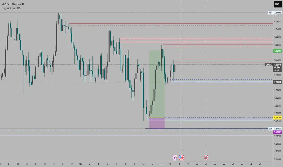
Wick SweepThe Wick Sweep indicator identifies potential trend reversal zones based on price action patterns and swing points. Specifically, it looks for "Wick Sweeps," a concept where the market temporarily breaks a swing low or high (creating a "wick"), only to reverse in the opposite direction. This pattern is often indicative of a market attempting to trap traders before making a larger move. The indicator marks these zones using dashed lines, helping traders spot key areas of potential price action.
Key Features:
* Swing Low and High Detection: The indicator identifies significant swing lows and highs within a user-defined period by employing Williams fractals.
* Wick Sweep Detection: Once a swing low or high is identified, the indicator looks for price movements that break through the low or high (creating a wick) and then reverses direction.
* Fractal Plotting: Optionally, the indicator plots fractal points (triangle shapes) on the chart when a swing low or high is detected. This can assist in visually identifying the potential wick sweep areas.
* Line Plotting: When a wick sweep is detected, a dashed line is drawn at the price level of the failed low or high, visually marking the potential reversal zone.
Inputs:
* Periods: The number of bars used to identify swing highs and lows. A higher value results in fewer, more significant swing points.
* Line Color: The color of the dashed lines drawn when a wick sweep is detected. Customize this to match your chart's theme or preferences.
* Show Fractals: A toggle that, when enabled, plots triangle shapes above and below bars indicating swing highs (up triangles) and swing lows (down triangles).
Functionality:
* Swing High and Low Calculation:
- The indicator calculates the swing low and swing high based on the periods input. A swing low is identified when the current low is the lowest within a range of (2 * periods + 1), with the lowest point being at the center of the period.
- Similarly, a swing high is identified when the current high is the highest within the same range.
* Wick Sweep Detection:
- Once a swing low or high is detected, the script looks for a potential wick. This happens when the price breaks the swing low or high and then reverses in the opposite direction.
- For a valid wick sweep, the price should briefly move beyond the identified swing point but then close in the opposite direction (i.e., a bullish reversal for a swing low and a bearish reversal for a swing high).
- A line is drawn at the price level of the failed low or high when a wick sweep is confirmed.
Confirmations for Reversal:
* The confirmation for a wick sweep requires that the price not only break the swing low/high but also close in the opposite direction (i.e., close above the low for a bullish reversal or close below the high for a bearish reversal).
* The confirmation is further refined by checking that the price movement is within a reasonable distance from the original swing point, which prevents the indicator from marking distant, unimportant price levels.
Additional Notes:
* The Wick Sweep indicator does not provide standalone trading signals; it is best used in conjunction with other technical analysis tools, such as trend analysis, oscillators, or volume indicators.
* The periods input can be adjusted based on the trader’s preferred level of sensitivity. A lower period value will result in more frequent swing points and potentially more signals, while a higher value will focus on more significant market swings.
* The indicator may work well in ranging markets where price tends to oscillate between key support and resistance levels.

OBV by readCrypto
-------------------------------------
OBV is used as a leading indicator to predict stock price movements by measuring changes in trading volume.
Reflecting the cumulative value of trading volume,
- When the price rises, if the trading volume increases, OBV rises,
- When the price falls, if the trading volume decreases, OBV falls.
Therefore, the movement of the OBV indicator must be checked along with the price movement, and it has the disadvantage of being unreliable for coins (tokens) with low trading volume.
---------------------------------------
(First interpretation method)
By adding a signal line for the OBV indicator,
- If the OBV indicator moves above the signal line, it is likely to show an upward trend,
- If the OBV indicator moves beyond the signal line, it is likely to show a downward trend.
This interpretation method is difficult to use in actual trading strategies because the OBV indicator often moves up and down repeatedly based on the signal line.
Therefore, it is recommended to use this interpretation method as reference when analyzing charts.
-------------------------------
(Second interpretation method)
Draw support and resistance lines based on the high and low points of the OBV indicator
- If the OBV indicator breaks through the previous high point, it is likely to show an upward trend,
- If the OBV indicator breaks through the previous low point, it is likely to show a downward trend.
This interpretation method is a bit more reliable than the first interpretation method, but it has the disadvantage of having to consider support and resistance lines separately based on the high and low points.
-
To compensate for this, a High line for the high point and a Low line for the low point were added.
- If the OBV indicator shows an upward breakout of each line (Low, HL2, High), the price is likely to rise,
- If the OBV indicator shows a downward breakout of each line (Low, HL2, High), the price is likely to fall.
-
Also, the Low and High lines can be interpreted like Bollinger Bands.
That is, if the Low and High lines show a contraction, the price is likely to move sideways, and if they show an expansion, the price is likely to show a trend.
Therefore, if the High line breaks upward in a contracted state,
- It is likely to show an upward trend,
- If the Low line breaks downward, it is likely to show a downward trend.
In an expanded state, you should focus on finding the point to realize profits rather than conducting new transactions.
--------------------------------
It is not easy to interpret the change in actual transaction volume and use it to create a trading strategy.
In particular, it is more difficult in the coin market where multiple exchanges are linked to show movements for one coin (token).
Therefore, the coin market is actively conducting transactions without referring to trading volume at all by following trends.
However, I think that if you interpret the change in trading volume and use it to find a trading point, it can help you find a more accurate trading point.
In that sense, I think that an indicator that adds the High and Low lines of the OBV indicator can be used as meaningful reference material.
-----------------------------------------------------------------
-------------------------------------
OBV는 거래량의 변화를 측정하여 주가 움직임을 예측하는 선행 지표로 활용됩니다.
거래량의 누적값을 반영하여
- 가격이 상승할 때 거래량이 증가면 OBV가 상승하고,
- 가격이 하락할 때 거래량이 줄면 OBV가 하락하게 됩니다.
따라서, 가격의 움직임과 함께 OBV 지표의 움직임을 확인하여야 하고 거래량이 적은 코인(토큰)에서는 신뢰성이 떨어지는 단점도 가지고 있습니다.
---------------------------------------
(첫번째 해석 방법)
OBV 지표에 대한 Signal선을 추가하여
- OBV 지표가 Signal선 이상에서 이동하게 되면 상승세를 보일 가능성이 높고,
- OBV 지표가 Signal선 이항에서 이동하게 되면 하락세를 보일 가능성이 높습니다.
이러한 해석 방법은 Signal선을 기준으로 OBV 지표가 반복적으로 위아래로 움직임을 보이는 경우가 많기 때문에 실제 거래 전략에 활용되기가 어려운 면이 있습니다.
따라서, 이러한 해설 방법은 차트 분석을 할 때 참고 자료로 활용하는 것이 좋습니다.
-------------------------------
(두번째 해석 방법)
OBV 지표의 고점과 저점을 기준하여 지지와 저항선을 그려
- OBV 지표가 이전 고점을 상향 돌파하면 상승세를 보일 가능성이 높고,
- OBV 지표가 이전 저점을 하향 돌파하면 하락세를 보일 가능성이 높습니다.
이러한 해석 방법은 첫번째 해석 방법보다 좀 더 신뢰성이 있는 방법이지만, 고점과 저점을 기준으로 지지와 저항선을 나누어 생각해야 하는 단점이 있습니다.
-
이를 보완하고자 고점에 대한 High선과 저점에 대한 Low선을 추가하였습니다.
- OBV 지표가 각 선(Low, HL2, High)을 상향 돌파하는 모습을 보이면 가격이 상승할 가능성이 높고,
- OBV 지표가 각 선(Low, HL2, High)을 하향 돌파하는 모습을 보이면 가격이 하락할 가능성이 높습니다.
-
또한, Low선과 High선을 볼린저밴드와 같이 해석할 수 있습니다.
즉, Low선과 High선이 수축하는 모습을 보이면 가격은 횡보할 가능성이 높고, 확장하는 모습을 보이면 가격은 추세를 나타낼 가능성이 높습니다.
따라서, 수축한 상태에서
- High선을 상향 돌파하게 되면 상승세를 나타낼 가능성이 높고,
- Low선을 하향 돌파하게 되면 하락세를 나타낼 가능성이 높습니다.
확장된 상태에서는 신규 거래를 진행하기 보다 수익 실현할 시점을 찾는데 집중해야 합니다.
--------------------------------
실제 거래량의 변화를 해석하여 거래 전략을 만드는데 활용하기가 쉽지 않습니다.
특히, 하나의 코인(토큰)에 대해서 여러 개의 거래소가 연동되어 움직임을 나타내는 코인 시장에서는 더욱 어려움이 있습니다.
따라서, 코인 시장은 추세 추종으로 아예 거래량을 참고하지 않고 거래를 진행하는 방법이 활성화되어 있기도 합니다.
하지만, 거래량의 변화를 해석하여 거래 시점을 찾는데 활용한다면 보다 정확한 거래 시점을 찾는데 도움을 받을 수 있다고 생각합니다.
그러한 의미에서 OBV 지표의 High선과 Low선을 추가한 지표가 의미 있는 참고 자료로 활용될 수 있다고 생각합니다.
-------------------------------------------------------------------

SCE Price Action SuiteThis is an indicator designed to use past market data to mark key price action levels as well as provide a different kind of insight. There are 8 different features in the script that users can turn on and off. This description will go in depth on all 8 with chart examples.
#1 Absorption Zones
I defined Absorption Zones as follows.
//----------------------------------------------
//---------------Absorption---------------------
//----------------------------------------------
box absorptionBox = na
absorptionBar = ta.highest(bodySize, absorptionLkb)
bsab = ta.barssince(bool(ta.change(absorptionBar)))
if bsab == 0 and upBar and showAbsorption
absorptionBox := box.new(left = bar_index - 1, top = close, right = bar_index + az_strcuture, bottom = open, border_color = color.rgb(0, 80, 75), border_width = boxLineSize, bgcolor = color.rgb(0, 80, 75))
absorptionBox
else if bsab == 0 and downBar and showAbsorption
absorptionBox := box.new(left = bar_index - 1, top = close, right = bar_index + az_strcuture, bottom = open, border_color = color.rgb(105, 15, 15), border_width = boxLineSize, bgcolor = color.rgb(105, 15, 15))
absorptionBox
What this means is that absorption bars are defined as the bars with the largest bodies over a selected lookback period. Those large bodies represent areas where price may react. I was inspired by the concept of a Fair Value Gap for this concept. In that body price may enter to be a point of support or resistance, market participants get “absorbed” in the area so price can continue in whichever direction.
#2 Candle Wick Theory/Strategy
I defined Candle Wick Theory/Strategy as follows.
//----------------------------------------------
//---------------Candle Wick--------------------
//----------------------------------------------
highWick = upBar ? high - close : downBar ? high - open : na
lowWick = upBar ? open - low : downBar ? close - low : na
upWick = upBar ? close + highWick : downBar ? open + highWick : na
downWick = upBar ? open - lowWick : downBar ? close - lowWick : na
downDelivery = upBar and downBar and high > upWick and highWick > lowWick and totalSize > totalSize and barstate.isconfirmed and session.ismarket
upDelivery = downBar and upBar and low < downWick and highWick < lowWick and totalSize > totalSize and barstate.isconfirmed and session.ismarket
line lG = na
line lE = na
line lR = na
bodyMidpoint = math.abs(body) / 2
upWickMidpoint = math.abs(upWickSize) / 2
downWickkMidpoint = math.abs(downWickSize) / 2
if upDelivery and showCdTheory
cpE = chart.point.new(time, bar_index - 1, downWickkMidpoint)
cpE2 = chart.point.new(time, bar_index + bl, downWickkMidpoint)
cpG = chart.point.new(time, bar_index + bl, downWickkMidpoint * (1 + tp))
cpR = chart.point.new(time, bar_index + bl, downWickkMidpoint * (1 - sl))
cpG1 = chart.point.new(time, bar_index - 1, downWickkMidpoint * (1 + tp))
cpR1 = chart.point.new(time, bar_index - 1, downWickkMidpoint * (1 - sl))
lG := line.new(cpG1, cpG, xloc.bar_index, extend.none, color.green, line.style_solid, 1)
lE := line.new(cpE, cpE2, xloc.bar_index, extend.none, color.white, line.style_solid, 1)
lR := line.new(cpR1, cpR, xloc.bar_index, extend.none, color.red, line.style_solid, 1)
lR
else if downDelivery and showCdTheory
cpE = chart.point.new(time, bar_index - 1, upWickMidpoint)
cpE2 = chart.point.new(time, bar_index + bl, upWickMidpoint)
cpG = chart.point.new(time, bar_index + bl, upWickMidpoint * (1 - tp))
cpR = chart.point.new(time, bar_index + bl, upWickMidpoint * (1 + sl))
cpG1 = chart.point.new(time, bar_index - 1, upWickMidpoint * (1 - tp))
cpR1 = chart.point.new(time, bar_index - 1, upWickMidpoint * (1 + sl))
lG := line.new(cpG1, cpG, xloc.bar_index, extend.none, color.green, line.style_solid, 1)
lE := line.new(cpE, cpE2, xloc.bar_index, extend.none, color.white, line.style_solid, 1)
lR := line.new(cpR1, cpR, xloc.bar_index, extend.none, color.red, line.style_solid, 1)
lR
First I get the size of the wicks for the top and bottoms of the candles. This depends on if the bar is red or green. If the bar is green the wick is the high minus the close, if red the high minus the open, and so on. Next, the script defines the upper and lower bounds of the wicks for further comparison. If the candle is green, it's the open price minus the bottom wick. If the candle is red, it's the close price minus the bottom wick, and so on. Next we have the condition for when this strategy is present.
Down delivery:
Occurs when the previous candle is green, the current candle is red, and:
The high of the current candle is above the upper wick of the previous candle.
The size of the current candle's top wick is greater than its bottom wick.
The total size of the previous candle is greater than the total size of the current candle.
The current bar is confirmed (barstate.isconfirmed).
The session is during market hours (session.ismarket).
Up delivery:
Occurs when the previous candle is red, the current candle is green, and:
The low of the current candle is below the lower wick of the previous candle.
The size of the current candle's bottom wick is greater than its top wick.
The total size of the previous candle is greater than the total size of the current candle.
The current bar is confirmed.
The session is during market hours
Then risk is plotted from the percentage that users can input from an ideal entry spot.
#3 Candle Size Theory
I defined Candle Size Theory as follows.
//----------------------------------------------
//---------------Candle displacement------------
//----------------------------------------------
line lECD = na
notableDown = bodySize > bodySize * candle_size_sensitivity and downBar and session.ismarket and barstate.isconfirmed
notableUp = bodySize > bodySize * candle_size_sensitivity and upBar and session.ismarket and barstate.isconfirmed
if notableUp and showCdSizeTheory
cpE = chart.point.new(time, bar_index - 1, close)
cpE2 = chart.point.new(time, bar_index + bl_strcuture, close)
lECD := line.new(cpE, cpE2, xloc.bar_index, extend.none, color.rgb(0, 80, 75), line.style_solid, 3)
lECD
else if notableDown and showCdSizeTheory
cpE = chart.point.new(time, bar_index - 1, close)
cpE2 = chart.point.new(time, bar_index + bl_strcuture, close)
lECD := line.new(cpE, cpE2, xloc.bar_index, extend.none, color.rgb(105, 15, 15), line.style_solid, 3)
lECD
This plots candles that are “notable” or out of the ordinary. Candles that are larger than the last by a value users get to specify. These candles' highs or lows, if they are green or red, act as levels for support or resistance.
#4 Candle Structure Theory
I defined Candle Structure Theory as follows.
//----------------------------------------------
//---------------Structure----------------------
//----------------------------------------------
breakDownStructure = low < low and low < low and high > high and upBar and downBar and upBar and downBar and session.ismarket and barstate.isconfirmed
breakUpStructure = low > low and low > low and high < high and downBar and upBar and downBar and upBar and session.ismarket and barstate.isconfirmed
if breakUpStructure and showStructureTheory
cpE = chart.point.new(time, bar_index - 1, close)
cpE2 = chart.point.new(time, bar_index + bl_strcuture, close)
lE := line.new(cpE, cpE2, xloc.bar_index, extend.none, color.teal, line.style_solid, 3)
lE
else if breakDownStructure and showStructureTheory
cpE = chart.point.new(time, bar_index - 1, open)
cpE2 = chart.point.new(time, bar_index + bl_strcuture, open)
lE := line.new(cpE, cpE2, xloc.bar_index, extend.none, color.red, line.style_solid, 3)
lE
It is a series of candles to create a notable event. 2 lower lows in a row, a lower high, then green bar, red bar, green bar is a structure for a breakdown. 2 higher lows in a row, a higher high, red bar, green bar, red bar for a break up.
#5 Candle Swing Structure Theory
I defined Candle Swing Structure Theory as follows.
//----------------------------------------------
//---------------Swing Structure----------------
//----------------------------------------------
line htb = na
line ltb = na
if totalSize * swing_struct_sense < totalSize and upBar and downBar and high > high and showSwingSturcture and session.ismarket and barstate.isconfirmed
cpS = chart.point.new(time, bar_index - 1, high)
cpE = chart.point.new(time, bar_index + bl_strcuture, high)
htb := line.new(cpS, cpE, xloc.bar_index, color = color.red, style = line.style_dashed)
htb
else if totalSize * swing_struct_sense < totalSize and downBar and upBar and low > low and showSwingSturcture and session.ismarket and barstate.isconfirmed
cpS = chart.point.new(time, bar_index - 1, low)
cpE = chart.point.new(time, bar_index + bl_strcuture, low)
ltb := line.new(cpS, cpE, xloc.bar_index, color = color.teal, style = line.style_dashed)
ltb
A bearish swing structure is defined as the last candle’s total size, times a scalar that the user can input, is less than the current candles. Like a size imbalance. The last bar must be green and this one red. The last high should also be less than this high. For a bullish swing structure the same size imbalance must be present, but we need a red bar then a green bar, and the last low higher than the current low.
#6 Fractal Boxes
I define the Fractal Boxes as follows
//----------------------------------------------
//---------------Fractal Boxes------------------
//----------------------------------------------
box b = na
int indexx = na
if bar_index % (n * 2) == 0 and session.ismarket and showBoxes
b := box.new(left = bar_index, top = topBox, right = bar_index + n, bottom = bottomBox, border_color = color.rgb(105, 15, 15), border_width = boxLineSize, bgcolor = na)
indexx := bar_index + 1
indexx
The idea of this strategy is that the market is fractal. It is considered impossible to be able to tell apart two different time frames from just the chart. So inside the chart there are many many breakouts and breakdowns happening as price bounces around. The boxes are there to give you the view from your timeframe if the market is in a range from a time frame that would be higher than it. Like if we are inside what a larger time frame candle’s range. If we break out or down from this, we might be able to trade it. Users can specify a lookback period and the box is that period’s, as an interval, high and low. I say as an interval because it is plotted every n * 2 bars. So we get a box, price moves, then a new box.
#7 Potential Move Width
I define the Potential Move Width as follows
//----------------------------------------------
//---------------Move width---------------------
//----------------------------------------------
velocity = V(n)
line lC = na
line l = na
line l2 = na
line l3 = na
line l4 = na
line l5 = na
line l6 = na
line l7 = na
line l8 = na
line lGFractal = na
line lRFractal = na
cp2 = chart.point.new(time, bar_index + n, close + velocity)
cp3 = chart.point.new(time, bar_index + n, close - velocity)
cp4 = chart.point.new(time, bar_index + n, close + velocity * 5)
cp5 = chart.point.new(time, bar_index + n, close - velocity * 5)
cp6 = chart.point.new(time, bar_index + n, close + velocity * 10)
cp7 = chart.point.new(time, bar_index + n, close - velocity * 10)
cp8 = chart.point.new(time, bar_index + n, close + velocity * 15)
cp9 = chart.point.new(time, bar_index + n, close - velocity * 15)
cpG = chart.point.new(time, bar_index + n, close + R)
cpR = chart.point.new(time, bar_index + n, close - R)
if ((bar_index + n) * 2 - bar_index) % n == 0 and session.ismarket and barstate.isconfirmed and showPredictionWidtn
cp = chart.point.new(time, bar_index, close)
cpG1 = chart.point.new(time, bar_index, close + R)
cpR1 = chart.point.new(time, bar_index, close - R)
l := line.new(cp, cp2, xloc.bar_index, extend.none, color.aqua, line.style_solid, 1)
l2 := line.new(cp, cp3, xloc.bar_index, extend.none, color.aqua, line.style_solid, 1)
l3 := line.new(cp, cp4, xloc.bar_index, extend.none, color.red, line.style_solid, 1)
l4 := line.new(cp, cp5, xloc.bar_index, extend.none, color.red, line.style_solid, 1)
l5 := line.new(cp, cp6, xloc.bar_index, extend.none, color.teal, line.style_solid, 1)
l6 := line.new(cp, cp7, xloc.bar_index, extend.none, color.teal, line.style_solid, 1)
l7 := line.new(cp, cp8, xloc.bar_index, extend.none, color.blue, line.style_solid, 1)
l8 := line.new(cp, cp9, xloc.bar_index, extend.none, color.blue, line.style_solid, 1)
l8
By using the past n bar’s velocity, or directional speed, every n * 2 bars. I can use it to scale the close value and get an estimate for how wide the next moves might be.
#8 Linear regression
//----------------------------------------------
//---------------Linear Regression--------------
//----------------------------------------------
lr = showLR ? ta.linreg(close, n, 0) : na
plot(lr, 'Linear Regression', color.blue)
I used TradingView’s built in linear regression to not reinvent the wheel. This is present to see past market strength of weakness from a different perspective.
User input
Users can control a lot about this script. For the strategy based plots you can enter what you want the risk to be in percentages. So the default 0.01 is 1%. You can also control how far forward the line goes.
Look back at where it is needed as well as line width for the Fractal Boxes are controllable. Also users can check on and off what they would like to see on the charts.
No indicator is 100% reliable, do not follow this one blindly. I encourage traders to make their own decisions and not trade solely based on technical indicators. I encourage constructive criticism in the comments below. Thank you.

lib_smcLibrary "lib_smc"
This is an adaptation of LuxAlgo's Smart Money Concepts indicator with numerous changes. Main changes include integration of object based plotting, plenty of performance improvements, live tracking of Order Blocks, integration of volume profiles to refine Order Blocks, and many more.
This is a library for developers, if you want this converted into a working strategy, let me know.
buffer(item, len, force_rotate)
Parameters:
item (float)
len (int)
force_rotate (bool)
buffer(item, len, force_rotate)
Parameters:
item (int)
len (int)
force_rotate (bool)
buffer(item, len, force_rotate)
Parameters:
item (Profile type from robbatt/lib_profile/32)
len (int)
force_rotate (bool)
swings(len)
INTERNAL: detect swing points (HH and LL) in given range
Parameters:
len (simple int) : range to check for new swing points
Returns: values are the price level where and if a new HH or LL was detected, else na
method init(this)
Namespace types: OrderBlockConfig
Parameters:
this (OrderBlockConfig)
method delete(this)
Namespace types: OrderBlock
Parameters:
this (OrderBlock)
method clear_broken(this, broken_buffer)
INTERNAL: delete internal order blocks box coordinates if top/bottom is broken
Namespace types: map
Parameters:
this (map)
broken_buffer (map)
Returns: any_bull_ob_broken, any_bear_ob_broken, broken signals are true if an according order block was broken/mitigated, broken contains the broken block(s)
create_ob(id, mode, start_t, start_i, top, end_t, end_i, bottom, break_price, early_confirmation_price, config, init_plot, force_overlay)
INTERNAL: set internal order block coordinates
Parameters:
id (int)
mode (int) : 1: bullish, -1 bearish block
start_t (int)
start_i (int)
top (float)
end_t (int)
end_i (int)
bottom (float)
break_price (float)
early_confirmation_price (float)
config (OrderBlockConfig)
init_plot (bool)
force_overlay (bool)
Returns: signals are true if an according order block was broken/mitigated
method align_to_profile(block, align_edge, align_break_price)
Namespace types: OrderBlock
Parameters:
block (OrderBlock)
align_edge (bool)
align_break_price (bool)
method create_profile(block, opens, tops, bottoms, closes, values, resolution, vah_pc, val_pc, args, init_calculated, init_plot, force_overlay)
Namespace types: OrderBlock
Parameters:
block (OrderBlock)
opens (array)
tops (array)
bottoms (array)
closes (array)
values (array)
resolution (int)
vah_pc (float)
val_pc (float)
args (ProfileArgs type from robbatt/lib_profile/32)
init_calculated (bool)
init_plot (bool)
force_overlay (bool)
method create_profile(block, resolution, vah_pc, val_pc, args, init_calculated, init_plot, force_overlay)
Namespace types: OrderBlock
Parameters:
block (OrderBlock)
resolution (int)
vah_pc (float)
val_pc (float)
args (ProfileArgs type from robbatt/lib_profile/32)
init_calculated (bool)
init_plot (bool)
force_overlay (bool)
track_obs(swing_len, hh, ll, top, btm, bull_bos_alert, bull_choch_alert, bear_bos_alert, bear_choch_alert, min_block_size, max_block_size, config_bull, config_bear, init_plot, force_overlay, enabled, extend_blocks, clear_broken_buffer_before, align_edge_to_value_area, align_break_price_to_poc, profile_args_bull, profile_args_bear, use_soft_confirm, soft_confirm_offset, use_retracements_with_FVG_out)
Parameters:
swing_len (int)
hh (float)
ll (float)
top (float)
btm (float)
bull_bos_alert (bool)
bull_choch_alert (bool)
bear_bos_alert (bool)
bear_choch_alert (bool)
min_block_size (float)
max_block_size (float)
config_bull (OrderBlockConfig)
config_bear (OrderBlockConfig)
init_plot (bool)
force_overlay (bool)
enabled (bool)
extend_blocks (simple bool)
clear_broken_buffer_before (simple bool)
align_edge_to_value_area (simple bool)
align_break_price_to_poc (simple bool)
profile_args_bull (ProfileArgs type from robbatt/lib_profile/32)
profile_args_bear (ProfileArgs type from robbatt/lib_profile/32)
use_soft_confirm (simple bool)
soft_confirm_offset (float)
use_retracements_with_FVG_out (simple bool)
method draw(this, config, extend_only)
Namespace types: OrderBlock
Parameters:
this (OrderBlock)
config (OrderBlockConfig)
extend_only (bool)
method draw(blocks, config)
INTERNAL: plot order blocks
Namespace types: array
Parameters:
blocks (array)
config (OrderBlockConfig)
method draw(blocks, config)
INTERNAL: plot order blocks
Namespace types: map
Parameters:
blocks (map)
config (OrderBlockConfig)
method cleanup(this, ob_bull, ob_bear)
removes all Profiles that are older than the latest OrderBlock from this profile buffer
Namespace types: array
Parameters:
this (array type from robbatt/lib_profile/32)
ob_bull (OrderBlock)
ob_bear (OrderBlock)
_plot_swing_points(mode, x, y, show_swing_points, linecolor_swings, keep_history, show_latest_swings_levels, trail_x, trail_y, trend)
INTERNAL: plot swing points
Parameters:
mode (int) : 1: bullish, -1 bearish block
x (int) : x-coordingate of swing point to plot (bar_index)
y (float) : y-coordingate of swing point to plot (price)
show_swing_points (bool) : switch to enable/disable plotting of swing point labels
linecolor_swings (color) : color for swing point labels and lates level lines
keep_history (bool) : weater to remove older swing point labels and only keep the most recent
show_latest_swings_levels (bool)
trail_x (int) : x-coordinate for latest swing point (bar_index)
trail_y (float) : y-coordinate for latest swing point (price)
trend (int) : the current trend 1: bullish, -1: bearish, to determine Strong/Weak Low/Highs
_pivot_lvl(mode, trend, hhll_x, hhll, super_hhll, filter_insignificant_internal_breaks)
INTERNAL: detect whether a structural level has been broken and if it was in trend direction (BoS) or against trend direction (ChoCh), also track the latest high and low swing points
Parameters:
mode (simple int) : detect 1: bullish, -1 bearish pivot points
trend (int) : current trend direction
hhll_x (int) : x-coordinate of newly detected hh/ll (bar_index)
hhll (float) : y-coordinate of newly detected hh/ll (price)
super_hhll (float) : level/y-coordinate of superior hhll (if this is an internal structure pivot level)
filter_insignificant_internal_breaks (bool) : if true pivot points / internal structure will be ignored where the wick in trend direction is longer than the opposite (likely to push further in direction of main trend)
Returns: coordinates of internal structure that has been broken (x,y): start of structure, (trail_x, trail_y): tracking hh/ll after structure break, (bos_alert, choch_alert): signal whether a structural level has been broken
_plot_structure(x, y, is_bos, is_choch, line_color, line_style, label_style, label_size, keep_history)
INTERNAL: plot structural breaks (BoS/ChoCh)
Parameters:
x (int) : x-coordinate of newly broken structure (bar_index)
y (float) : y-coordinate of newly broken structure (price)
is_bos (bool) : whether this structural break was in trend direction
is_choch (bool) : whether this structural break was against trend direction
line_color (color) : color for the line connecting the structural level and the breaking candle
line_style (string) : style (line.style_dashed/solid) for the line connecting the structural level and the breaking candle
label_style (string) : style (label.style_label_down/up) for the label above/below the line connecting the structural level and the breaking candle
label_size (string) : size (size.small/tiny) for the label above/below the line connecting the structural level and the breaking candle
keep_history (bool) : weater to remove older swing point labels and only keep the most recent
structure_values(length, super_hh, super_ll, filter_insignificant_internal_breaks)
detect (and plot) structural breaks and the resulting new trend
Parameters:
length (simple int) : lookback period for swing point detection
super_hh (float) : level/y-coordinate of superior hh (for internal structure detection)
super_ll (float) : level/y-coordinate of superior ll (for internal structure detection)
filter_insignificant_internal_breaks (bool) : if true pivot points / internal structure will be ignored where the wick in trend direction is longer than the opposite (likely to push further in direction of main trend)
Returns: trend: direction 1:bullish -1:bearish, (bull_bos_alert, bull_choch_alert, top_x, top_y, trail_up_x, trail_up): whether and which level broke in a bullish direction, trailing high, (bbear_bos_alert, bear_choch_alert, tm_x, btm_y, trail_dn_x, trail_dn): same in bearish direction
structure_plot(trend, bull_bos_alert, bull_choch_alert, top_x, top_y, trail_up_x, trail_up, hh, bear_bos_alert, bear_choch_alert, btm_x, btm_y, trail_dn_x, trail_dn, ll, color_bull, color_bear, show_swing_points, show_latest_swings_levels, show_bos, show_choch, line_style, label_size, keep_history)
detect (and plot) structural breaks and the resulting new trend
Parameters:
trend (int) : crrent trend 1: bullish, -1: bearish
bull_bos_alert (bool) : if there was a bullish bos alert -> plot it
bull_choch_alert (bool) : if there was a bullish choch alert -> plot it
top_x (int) : latest shwing high x
top_y (float) : latest swing high y
trail_up_x (int) : trailing high x
trail_up (float) : trailing high y
hh (float) : if there was a higher high
bear_bos_alert (bool) : if there was a bearish bos alert -> plot it
bear_choch_alert (bool) : if there was a bearish chock alert -> plot it
btm_x (int) : latest swing low x
btm_y (float) : latest swing low y
trail_dn_x (int) : trailing low x
trail_dn (float) : trailing low y
ll (float) : if there was a lower low
color_bull (color) : color for bullish BoS/ChoCh levels
color_bear (color) : color for bearish BoS/ChoCh levels
show_swing_points (bool) : whether to plot swing point labels
show_latest_swings_levels (bool) : whether to track and plot latest swing point levels with lines
show_bos (bool) : whether to plot BoS levels
show_choch (bool) : whether to plot ChoCh levels
line_style (string) : whether to plot BoS levels
label_size (string) : label size of plotted BoS/ChoCh levels
keep_history (bool) : weater to remove older swing point labels and only keep the most recent
structure(length, color_bull, color_bear, super_hh, super_ll, filter_insignificant_internal_breaks, show_swing_points, show_latest_swings_levels, show_bos, show_choch, line_style, label_size, keep_history, enabled)
detect (and plot) structural breaks and the resulting new trend
Parameters:
length (simple int) : lookback period for swing point detection
color_bull (color) : color for bullish BoS/ChoCh levels
color_bear (color) : color for bearish BoS/ChoCh levels
super_hh (float) : level/y-coordinate of superior hh (for internal structure detection)
super_ll (float) : level/y-coordinate of superior ll (for internal structure detection)
filter_insignificant_internal_breaks (bool) : if true pivot points / internal structure will be ignored where the wick in trend direction is longer than the opposite (likely to push further in direction of main trend)
show_swing_points (bool) : whether to plot swing point labels
show_latest_swings_levels (bool) : whether to track and plot latest swing point levels with lines
show_bos (bool) : whether to plot BoS levels
show_choch (bool) : whether to plot ChoCh levels
line_style (string) : whether to plot BoS levels
label_size (string) : label size of plotted BoS/ChoCh levels
keep_history (bool) : weater to remove older swing point labels and only keep the most recent
enabled (bool)
_check_equal_level(mode, len, eq_threshold, enabled)
INTERNAL: detect equal levels (double top/bottom)
Parameters:
mode (int) : detect 1: bullish/high, -1 bearish/low pivot points
len (int) : lookback period for equal level (swing point) detection
eq_threshold (float) : maximum price offset for a level to be considered equal
enabled (bool)
Returns: eq_alert whether an equal level was detected and coordinates of the first and the second level/swing point
_plot_equal_level(show_eq, x1, y1, x2, y2, label_txt, label_style, label_size, line_color, line_style, keep_history)
INTERNAL: plot equal levels (double top/bottom)
Parameters:
show_eq (bool) : whether to plot the level or not
x1 (int) : x-coordinate of the first level / swing point
y1 (float) : y-coordinate of the first level / swing point
x2 (int) : x-coordinate of the second level / swing point
y2 (float) : y-coordinate of the second level / swing point
label_txt (string) : text for the label above/below the line connecting the equal levels
label_style (string) : style (label.style_label_down/up) for the label above/below the line connecting the equal levels
label_size (string) : size (size.tiny) for the label above/below the line connecting the equal levels
line_color (color) : color for the line connecting the equal levels (and it's label)
line_style (string) : style (line.style_dotted) for the line connecting the equal levels
keep_history (bool) : weater to remove older swing point labels and only keep the most recent
equal_levels_values(len, threshold, enabled)
detect (and plot) equal levels (double top/bottom), returns coordinates
Parameters:
len (int) : lookback period for equal level (swing point) detection
threshold (float) : maximum price offset for a level to be considered equal
enabled (bool) : whether detection is enabled
Returns: (eqh_alert, eqh_x1, eqh_y1, eqh_x2, eqh_y2) whether an equal high was detected and coordinates of the first and the second level/swing point, (eql_alert, eql_x1, eql_y1, eql_x2, eql_y2) same for equal lows
equal_levels_plot(eqh_x1, eqh_y1, eqh_x2, eqh_y2, eql_x1, eql_y1, eql_x2, eql_y2, color_eqh, color_eql, show, keep_history)
detect (and plot) equal levels (double top/bottom), returns coordinates
Parameters:
eqh_x1 (int) : coordinates of first point of equal high
eqh_y1 (float) : coordinates of first point of equal high
eqh_x2 (int) : coordinates of second point of equal high
eqh_y2 (float) : coordinates of second point of equal high
eql_x1 (int) : coordinates of first point of equal low
eql_y1 (float) : coordinates of first point of equal low
eql_x2 (int) : coordinates of second point of equal low
eql_y2 (float) : coordinates of second point of equal low
color_eqh (color) : color for the line connecting the equal highs (and it's label)
color_eql (color) : color for the line connecting the equal lows (and it's label)
show (bool) : whether plotting is enabled
keep_history (bool) : weater to remove older swing point labels and only keep the most recent
Returns: (eqh_alert, eqh_x1, eqh_y1, eqh_x2, eqh_y2) whether an equal high was detected and coordinates of the first and the second level/swing point, (eql_alert, eql_x1, eql_y1, eql_x2, eql_y2) same for equal lows
equal_levels(len, threshold, color_eqh, color_eql, enabled, show, keep_history)
detect (and plot) equal levels (double top/bottom)
Parameters:
len (int) : lookback period for equal level (swing point) detection
threshold (float) : maximum price offset for a level to be considered equal
color_eqh (color) : color for the line connecting the equal highs (and it's label)
color_eql (color) : color for the line connecting the equal lows (and it's label)
enabled (bool) : whether detection is enabled
show (bool) : whether plotting is enabled
keep_history (bool) : weater to remove older swing point labels and only keep the most recent
Returns: (eqh_alert) whether an equal high was detected, (eql_alert) same for equal lows
_detect_fvg(mode, enabled, o, h, l, c, filter_insignificant_fvgs, change_tf)
INTERNAL: detect FVG (fair value gap)
Parameters:
mode (int) : detect 1: bullish, -1 bearish gaps
enabled (bool) : whether detection is enabled
o (float) : reference source open
h (float) : reference source high
l (float) : reference source low
c (float) : reference source close
filter_insignificant_fvgs (bool) : whether to calculate and filter small/insignificant gaps
change_tf (bool) : signal when the previous reference timeframe closed, triggers new calculation
Returns: whether a new FVG was detected and its top/mid/bottom levels
_clear_broken_fvg(mode, upper_boxes, lower_boxes)
INTERNAL: clear mitigated FVGs (fair value gaps)
Parameters:
mode (int) : detect 1: bullish, -1 bearish gaps
upper_boxes (array) : array that stores the upper parts of the FVG boxes
lower_boxes (array) : array that stores the lower parts of the FVG boxes
_plot_fvg(mode, show, top, mid, btm, border_color, extend_box)
INTERNAL: plot (and clear broken) FVG (fair value gap)
Parameters:
mode (int) : plot 1: bullish, -1 bearish gap
show (bool) : whether plotting is enabled
top (float) : top level of fvg
mid (float) : center level of fvg
btm (float) : bottom level of fvg
border_color (color) : color for the FVG box
extend_box (int) : how many bars into the future the FVG box should be extended after detection
fvgs_values(o, h, l, c, filter_insignificant_fvgs, change_tf, enabled)
detect (and plot / clear broken) FVGs (fair value gaps), and return alerts and level values
Parameters:
o (float) : reference source open
h (float) : reference source high
l (float) : reference source low
c (float) : reference source close
filter_insignificant_fvgs (bool) : whether to calculate and filter small/insignificant gaps
change_tf (bool) : signal when the previous reference timeframe closed, triggers new calculation
enabled (bool) : whether detection is enabled
Returns: (bullish_fvg_alert, bull_top, bull_mid, bull_btm): whether a new bullish FVG was detected and its top/mid/bottom levels, (bearish_fvg_alert, bear_top, bear_mid, bear_btm): same for bearish FVGs
fvgs_plot(bullish_fvg_alert, bull_top, bull_mid, bull_btm, bearish_fvg_alert, bear_top, bear_mid, bear_btm, color_bull, color_bear, extend_box, show)
Parameters:
bullish_fvg_alert (bool)
bull_top (float)
bull_mid (float)
bull_btm (float)
bearish_fvg_alert (bool)
bear_top (float)
bear_mid (float)
bear_btm (float)
color_bull (color) : color for bullish FVG boxes
color_bear (color) : color for bearish FVG boxes
extend_box (int) : how many bars into the future the FVG box should be extended after detection
show (bool) : whether plotting is enabled
Returns: (bullish_fvg_alert, bull_top, bull_mid, bull_btm): whether a new bullish FVG was detected and its top/mid/bottom levels, (bearish_fvg_alert, bear_top, bear_mid, bear_btm): same for bearish FVGs
fvgs(o, h, l, c, filter_insignificant_fvgs, change_tf, color_bull, color_bear, extend_box, enabled, show)
detect (and plot / clear broken) FVGs (fair value gaps)
Parameters:
o (float) : reference source open
h (float) : reference source high
l (float) : reference source low
c (float) : reference source close
filter_insignificant_fvgs (bool) : whether to calculate and filter small/insignificant gaps
change_tf (bool) : signal when the previous reference timeframe closed, triggers new calculation
color_bull (color) : color for bullish FVG boxes
color_bear (color) : color for bearish FVG boxes
extend_box (int) : how many bars into the future the FVG box should be extended after detection
enabled (bool) : whether detection is enabled
show (bool) : whether plotting is enabled
Returns: (bullish_fvg_alert): whether a new bullish FVG was detected, (bearish_fvg_alert): same for bearish FVGs
OrderBlock
Fields:
id (series int)
dir (series int)
left_top (chart.point)
right_bottom (chart.point)
break_price (series float)
early_confirmation_price (series float)
ltf_high (array)
ltf_low (array)
ltf_volume (array)
plot (Box type from robbatt/lib_plot_objects/49)
profile (Profile type from robbatt/lib_profile/32)
trailing (series bool)
extending (series bool)
awaiting_confirmation (series bool)
touched_break_price_before_confirmation (series bool)
soft_confirmed (series bool)
has_fvg_out (series bool)
hidden (series bool)
broken (series bool)
OrderBlockConfig
Fields:
show (series bool)
show_last (series int)
show_id (series bool)
show_profile (series bool)
args (BoxArgs type from robbatt/lib_plot_objects/49)
txt (series string)
txt_args (BoxTextArgs type from robbatt/lib_plot_objects/49)
delete_when_broken (series bool)
broken_args (BoxArgs type from robbatt/lib_plot_objects/49)
broken_txt (series string)
broken_txt_args (BoxTextArgs type from robbatt/lib_plot_objects/49)
broken_profile_args (ProfileArgs type from robbatt/lib_profile/32)
use_profile (series bool)
profile_args (ProfileArgs type from robbatt/lib_profile/32)