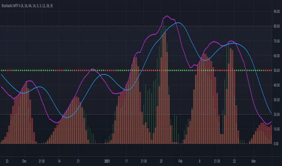
Stochastic MTF IICombines Stochastics, RSI and MACD Histogram to give a complete picture of the momentum.
The main two lines are stochastics from the higher time frame(current time frame* 4).
The red columns are stochastic of macd histogram.
The green histogram is the stochastic rsi of price.
The dots at 50 line is the correlation between price and macd+rsi combo.
Cari skrip untuk "histogram"
Power Bar [racer8]Introduction: 🌟
The Power Bar indicator is a powerful volatility indicator that can detect power bars 💪. A power bar is just a really big price bar that forms after a price base. A price base is chart pattern consisting of many low volatility price bars (bars that have small ranges). To detect such powerful bars, the PB indicator uses the following formula:
PB = ( Absolute value of current close - previous close ) / ( Previous price range over n periods )
Looking at the formula, you can see that PB compares the current change in closing price to the n-period base pattern's range. Strong PB values are typically greater than a value of 1. If n periods = 10, the indicator will look back 11 periods. The 11 periods includes the 10-period base plus the current price bar. 10 periods is the default setting for the indicator.
After the calculation, PB is then plotted as a histogram. Along with the histogram, a horizontal dashed line is also plotted.
PB's other setting controls the dashed line's level. This level is preset at a default value of 1. The dashed line is just a way to filter out weak PB values, and to generate signals. A signal is generated when the PB histogram is above the dashed line.
Objective: 🤔
This indicator shall prove very useful to you if your main objective is to trade only the best chart pattern in the market...and the base pattern is one of the best, if not the best chart pattern that exists today. This indicator is a mechanical way of detecting the chart pattern.
Enjoy! 🥳

MACD ProMoving average convergence divergence pro.
Original MACD with new features, Including...
1. Three different modes.
Basic, Logarithmic, Percent (calculates difference of oscillator MAs in percent)
2. Additional moving averages for oscillator, signal and even histogram.
EMA, WMA (linearly weighted), LMA (logarithmically weighted), SMA
Volume Weighted RMA (I've been suggested to make a MACD with the VWEMA that I published recently but that was too fast, this almost 2 times slower because of using RMA instead of EMA)
VWRMA(s) (an alternative for VWRMA which uses candle formation to simulate the volume, can be useful when volume is not provided for the symbol or it is not proper)
And DEMA (Double Exponential MA)
3. Signal Displacement.
If you want to add some delay to signal, could help for extra confirmation of center crosses and removal of some falss ones.
4. Histogram Smoother.
For those who like the smooth curves. Can deliver a cleaner histogram even in volatile markets.
5. Bar color for more fun.

DMI Candle ColorPaints the color of the candles in accordance with the DMI Histogram. Two colors are supported - one for DMI Histogram above zero and one for DMI Histogram below zero. Inputs for ADX Smoothing and DI Length are also supported.

EMA Slope - ValenteThis indicator will show you the EMA SLOPE as a HISTOGRAM.
Este indicador mostra a INCLINACAO da EMA como um HISTOGRAMA

Weighted Volume ROC OscillatorWeighted Volume ROC Oscillator (WVRO | MisinkoMaster)
The Weighted Volume ROC Oscillator is a sophisticated trend-following tool that leverages a volume-weighted Rate of Change (ROC) calculation on a double-smoothed source. Designed to capture both trend direction and strength with minimal noise, this oscillator also highlights potential reversal points, making it an effective tool for fast-moving markets like ETHUSD.
By combining volume weighting with advanced smoothing techniques, the WVRO provides a responsive yet stable indicator to help traders make more informed decisions during trending conditions.
🔍 Concept & Idea
The core idea behind the WVRO is to develop a high-speed oscillator capable of smoothly following trends while remaining sensitive to rapid changes. The ROC is a natural choice for momentum measurement, but raw ROC alone can be noisy.
To improve stability and responsiveness:
The input source is smoothed twice using Weighted Moving Averages (WMA) with a length proportional to the square root of the user-defined length, reducing noise while preserving fast reactions.
The ROC is then weighted by volume to emphasize price movements during high-volume periods, increasing the significance of meaningful trades.
Finally, a volume-weighted average of the ROC is calculated to normalize the signal.
This combination balances smoothness and speed, improving signal clarity in trending markets.
⚙️ How It Works
Double WMA Smoothing of Source:
First, apply a WMA with length √len to the selected source to filter noise but retain responsiveness.
Apply a second WMA with the same length to the first smoothed series for additional smoothing.
Volume-Weighted ROC Calculation:
Calculate ROC on the double-smoothed source over one bar.
Multiply the ROC by the current volume, weighting price changes by trading activity.
Normalization and Oscillator Computation:
Calculate an Exponential Moving Average (EMA) of the volume-weighted ROC over the full length.
Divide by the sum of volume over the same length to normalize, then scale to a range centered near zero.
Trend Logic:
Positive WVRO values indicate bullish momentum (trend up).
Negative values indicate bearish momentum (trend down).
Momentum Divergence:
The difference between the current WVRO and its prior value is smoothed with EMA and plotted as a histogram to help identify potential momentum shifts and reversals.
🧩 Inputs Overview
Oscillator Length – Controls the main smoothing and lookback length of the oscillator (default 17).
Source – The price source used for calculation, defaulting to the average of high, low, close, and close (hlcc4).
📌 Usage Notes
Responsive Yet Smooth: The double WMA smoothing ensures the oscillator is less prone to noise but remains quick to react to market changes.
Volume Weighting: Emphasizes price moves on higher volume bars, improving signal reliability in volatile markets.
Trend Identification: Positive and negative readings provide clear trend signals, while divergence histograms highlight potential turning points.
Visual Clarity: Color-coded plots and background highlighting assist quick interpretation.
Optimized for ETHUSD: Especially effective in high-liquidity, high-volatility assets like Ethereum.
Complement with Other Tools: Use alongside price action or other indicators to confirm trends and entry/exit points.
Backtest and Validate: Always validate settings on your chosen asset and timeframe before live use.
⚠️ Disclaimer
This indicator is for educational and analytical purposes only and does not constitute financial advice. Trading involves significant risk, and users should perform due diligence before trading.
Enjoy enhanced trend following with the Weighted Volume ROC Oscillator!

SpatialIndexYou can start using this now by inserthing this at the top of your indicator/strategy/library.
import ArunaReborn/SpatialIndex/1 as SI
Overview
SpatialIndex is a high-performance Pine Script library that implements price-bucketed spatial indexing for efficient proximity queries on large datasets. Instead of scanning through hundreds or thousands of items linearly (O(n)), this library provides O(k) bucket lookup where k is typically just a handful of buckets, dramatically improving performance for price-based filtering operations.
This library works with any data type through index-based references, making it universally applicable for support/resistance levels, pivot points, order zones, pattern detection points, Fair Value Gaps, and any other price-based data that needs frequent proximity queries.
Why This Library Exists
The Problem
When building advanced technical indicators that track large numbers of price levels (support/resistance zones, pivot points, order blocks, etc.), you often need to answer questions like:
- *"Which levels are within 5% of the current price?"*
- *"What zones overlap with this price range?"*
- *"Are there any significant levels near my entry point?"*
The naive approach is to loop through every single item and check its price. For 500 levels across multiple timeframes, this means 500 comparisons every bar . On instruments with thousands of historical bars, this quickly becomes a performance bottleneck that can cause scripts to time out or lag.
The Solution
SpatialIndex solves this by organizing items into price buckets —like filing cabinets organized by price range. When you query for items near $50,000, the library only looks in the relevant buckets (e.g., $49,000-$51,000 range), ignoring all other price regions entirely.
Performance Example:
- Linear scan: Check 500 items = 500 comparisons per query
- Spatial index: Check 3-5 buckets with ~10 items each = 30-50 comparisons per query
- Result: 10-16x faster queries
Key Features
Core Capabilities
- ✅ Generic Design : Works with any data type via index references
- ✅ Multiple Index Strategies : Fixed bucket size or ATR-based dynamic sizing
- ✅ Range Support : Index items that span price ranges (zones, gaps, channels)
- ✅ Efficient Queries : O(k) bucket lookup instead of O(n) linear scan
- ✅ Multiple Query Types : Proximity percentage, fixed range, exact price with tolerance
- ✅ Dynamic Updates : Add, remove, update items in O(1) time
- ✅ Batch Operations : Efficient bulk removal and reindexing
- ✅ Query Caching : Optional caching for repeated queries within same bar
- ✅ Statistics & Debugging : Built-in stats and diagnostic functions
### Advanced Features
- ATR-Based Bucketing : Automatically adjusts bucket sizes based on volatility
- Multi-Bucket Spanning : Items that span ranges are indexed in all overlapping buckets
- Reindexing Support : Handles array removals with automatic index shifting
- Cache Management : Configurable query caching with automatic invalidation
- Empty Bucket Cleanup : Automatically removes empty buckets to minimize memory
How It Works
The Bucketing Concept
Think of price space as divided into discrete buckets, like a histogram:
```
Price Range: $98-$100 $100-$102 $102-$104 $104-$106 $106-$108
Bucket Key: 49 50 51 52 53
Items:
```
When you query for items near $103:
1. Calculate which buckets overlap the $101.50-$104.50 range (keys 50, 51, 52)
2. Return items from only those buckets:
3. Never check items in buckets 49 or 53
Bucket Size Selection
Fixed Size Mode:
```pine
var SI.SpatialBucket index = SI.newSpatialBucket(2.0) // $2 per bucket
```
- Good for: Instruments with stable price ranges
- Example: For stocks trading at $100, 2.0 = 2% increments
ATR-Based Mode:
```pine
float atr = ta.atr(14)
var SI.SpatialBucket index = SI.newSpatialBucketATR(1.0, atr) // 1x ATR per bucket
SI.updateATR(index, atr) // Update each bar
```
- Good for: Instruments with varying volatility
- Adapts automatically to market conditions
- 1.0 multiplier = one bucket spans one ATR unit
Optimal Bucket Size:
The library includes a helper function to calculate optimal size:
```pine
float optimalSize = SI.calculateOptimalBucketSize(close, 5.0) // For 5% proximity queries
```
This ensures queries span approximately 3 buckets for optimal performance.
Index-Based Architecture
The library doesn't store your actual data—it only stores indices that point to your external arrays:
```pine
// Your data
var array levels = array.new()
var array types = array.new()
var array ages = array.new()
// Your index
var SI.SpatialBucket index = SI.newSpatialBucket(2.0)
// Add a level
array.push(levels, 50000.0)
array.push(types, "support")
array.push(ages, 0)
SI.add(index, array.size(levels) - 1, 50000.0) // Store index 0
// Query near current price
SI.QueryResult result = SI.queryProximity(index, close, 5.0)
for idx in result.indices
float level = array.get(levels, idx)
string type = array.get(types, idx)
// Work with your actual data
```
This design means:
- ✅ Works with any data structure you define
- ✅ No data duplication
- ✅ Minimal memory footprint
- ✅ Full control over your data
---
Usage Guide
Basic Setup
```pine
// Import library
import username/SpatialIndex/1 as SI
// Create index
var SI.SpatialBucket index = SI.newSpatialBucket(2.0)
// Your data arrays
var array supportLevels = array.new()
var array touchCounts = array.new()
```
Adding Items
Single Price Point:
```pine
// Add a support level at $50,000
array.push(supportLevels, 50000.0)
array.push(touchCounts, 1)
int levelIdx = array.size(supportLevels) - 1
SI.add(index, levelIdx, 50000.0)
```
Price Range (Zones/Gaps):
```pine
// Add a resistance zone from $51,000 to $52,000
array.push(zoneBottoms, 51000.0)
array.push(zoneTops, 52000.0)
int zoneIdx = array.size(zoneBottoms) - 1
SI.addRange(index, zoneIdx, 51000.0, 52000.0) // Indexed in all overlapping buckets
```
Querying Items
Proximity Query (Percentage):
```pine
// Find all levels within 5% of current price
SI.QueryResult result = SI.queryProximity(index, close, 5.0)
if array.size(result.indices) > 0
for idx in result.indices
float level = array.get(supportLevels, idx)
// Process nearby level
```
Fixed Range Query:
```pine
// Find all items between $49,000 and $51,000
SI.QueryResult result = SI.queryRange(index, 49000.0, 51000.0)
```
Exact Price with Tolerance:
```pine
// Find items at exactly $50,000 +/- $100
SI.QueryResult result = SI.queryAt(index, 50000.0, 100.0)
```
Removing Items
Safe Removal Pattern:
```pine
SI.QueryResult result = SI.queryProximity(index, close, 5.0)
if array.size(result.indices) > 0
// IMPORTANT: Sort descending to safely remove from arrays
array sorted = SI.sortIndicesDescending(result)
for idx in sorted
// Remove from index
SI.remove(index, idx)
// Remove from your data arrays
array.remove(supportLevels, idx)
array.remove(touchCounts, idx)
// Reindex to maintain consistency
SI.reindexAfterRemoval(index, idx)
```
Batch Removal (More Efficient):
```pine
// Collect indices to remove
array toRemove = array.new()
for i = 0 to array.size(supportLevels) - 1
if array.get(touchCounts, i) > 10 // Remove old levels
array.push(toRemove, i)
// Remove in descending order from data arrays
array sorted = array.copy(toRemove)
array.sort(sorted, order.descending)
for idx in sorted
SI.remove(index, idx)
array.remove(supportLevels, idx)
array.remove(touchCounts, idx)
// Batch reindex (much faster than individual reindexing)
SI.reindexAfterBatchRemoval(index, toRemove)
```
Updating Items
```pine
// Update a level's price (e.g., after refinement)
float newPrice = 50100.0
SI.update(index, levelIdx, newPrice)
array.set(supportLevels, levelIdx, newPrice)
// Update a zone's range
SI.updateRange(index, zoneIdx, 51000.0, 52500.0)
array.set(zoneBottoms, zoneIdx, 51000.0)
array.set(zoneTops, zoneIdx, 52500.0)
```
Query Caching
For repeated queries within the same bar:
```pine
// Create cache (persistent)
var SI.CachedQuery cache = SI.newCachedQuery()
// Cached query (returns cached result if parameters match)
SI.QueryResult result = SI.queryProximityCached(
index,
cache,
close,
5.0, // proximity%
1 // cache duration in bars
)
// Invalidate cache when index changes significantly
if bigChangeDetected
SI.invalidateCache(cache)
```
---
Practical Examples
Example 1: Support/Resistance Finder
```pine
//@version=6
indicator("S/R with Spatial Index", overlay=true)
import username/SpatialIndex/1 as SI
// Data storage
var array levels = array.new()
var array types = array.new() // "support" or "resistance"
var array touches = array.new()
var array ages = array.new()
// Spatial index
var SI.SpatialBucket index = SI.newSpatialBucket(close * 0.02) // 2% buckets
// Detect pivots
bool isPivotHigh = ta.pivothigh(high, 5, 5)
bool isPivotLow = ta.pivotlow(low, 5, 5)
// Add new levels
if isPivotHigh
array.push(levels, high )
array.push(types, "resistance")
array.push(touches, 1)
array.push(ages, 0)
SI.add(index, array.size(levels) - 1, high )
if isPivotLow
array.push(levels, low )
array.push(types, "support")
array.push(touches, 1)
array.push(ages, 0)
SI.add(index, array.size(levels) - 1, low )
// Find nearby levels (fast!)
SI.QueryResult nearby = SI.queryProximity(index, close, 3.0) // Within 3%
// Process nearby levels
for idx in nearby.indices
float level = array.get(levels, idx)
string type = array.get(types, idx)
// Check for touch
if type == "support" and low <= level and low > level
array.set(touches, idx, array.get(touches, idx) + 1)
else if type == "resistance" and high >= level and high < level
array.set(touches, idx, array.get(touches, idx) + 1)
// Age and cleanup old levels
for i = array.size(ages) - 1 to 0
array.set(ages, i, array.get(ages, i) + 1)
// Remove levels older than 500 bars or with 5+ touches
if array.get(ages, i) > 500 or array.get(touches, i) >= 5
SI.remove(index, i)
array.remove(levels, i)
array.remove(types, i)
array.remove(touches, i)
array.remove(ages, i)
SI.reindexAfterRemoval(index, i)
// Visualization
for idx in nearby.indices
line.new(bar_index, array.get(levels, idx), bar_index + 10, array.get(levels, idx),
color=array.get(types, idx) == "support" ? color.green : color.red)
```
Example 2: Multi-Timeframe Zone Detector
```pine
//@version=6
indicator("MTF Zones", overlay=true)
import username/SpatialIndex/1 as SI
// Store zones from multiple timeframes
var array zoneBottoms = array.new()
var array zoneTops = array.new()
var array zoneTimeframes = array.new()
// ATR-based spatial index for adaptive bucketing
var SI.SpatialBucket index = SI.newSpatialBucketATR(1.0, ta.atr(14))
SI.updateATR(index, ta.atr(14)) // Update bucket size with volatility
// Request higher timeframe data
= request.security(syminfo.tickerid, "240", )
// Detect HTF zones
if not na(htf_high) and not na(htf_low)
float zoneTop = htf_high
float zoneBottom = htf_low * 0.995 // 0.5% zone thickness
// Check if zone already exists nearby
SI.QueryResult existing = SI.queryRange(index, zoneBottom, zoneTop)
if array.size(existing.indices) == 0 // No overlapping zones
// Add new zone
array.push(zoneBottoms, zoneBottom)
array.push(zoneTops, zoneTop)
array.push(zoneTimeframes, "4H")
int idx = array.size(zoneBottoms) - 1
SI.addRange(index, idx, zoneBottom, zoneTop)
// Query zones near current price
SI.QueryResult nearbyZones = SI.queryProximity(index, close, 2.0) // Within 2%
// Highlight nearby zones
for idx in nearbyZones.indices
box.new(bar_index - 50, array.get(zoneBottoms, idx),
bar_index, array.get(zoneTops, idx),
bgcolor=color.new(color.blue, 90))
```
### Example 3: Performance Comparison
```pine
//@version=6
indicator("Spatial Index Performance Test")
import username/SpatialIndex/1 as SI
// Generate 500 random levels
var array levels = array.new()
var SI.SpatialBucket index = SI.newSpatialBucket(close * 0.02)
if bar_index == 0
for i = 0 to 499
float randomLevel = close * (0.9 + math.random() * 0.2) // +/- 10%
array.push(levels, randomLevel)
SI.add(index, i, randomLevel)
// Method 1: Linear scan (naive approach)
int linearCount = 0
float proximityPct = 5.0
float lowBand = close * (1 - proximityPct/100)
float highBand = close * (1 + proximityPct/100)
for i = 0 to array.size(levels) - 1
float level = array.get(levels, i)
if level >= lowBand and level <= highBand
linearCount += 1
// Method 2: Spatial index query
SI.QueryResult result = SI.queryProximity(index, close, proximityPct)
int spatialCount = array.size(result.indices)
// Compare performance
plot(result.queryCount, "Items Examined (Spatial)", color=color.green)
plot(linearCount, "Items Examined (Linear)", color=color.red)
plot(spatialCount, "Results Found", color=color.blue)
// Spatial index typically examines 10-50 items vs 500 for linear scan!
```
API Reference Summary
Initialization
- `newSpatialBucket(bucketSize)` - Fixed bucket size
- `newSpatialBucketATR(atrMultiplier, atrValue)` - ATR-based buckets
- `updateATR(sb, newATR)` - Update ATR for dynamic sizing
Adding Items
- `add(sb, itemIndex, price)` - Add item at single price point
- `addRange(sb, itemIndex, priceBottom, priceTop)` - Add item spanning range
Querying
- `queryProximity(sb, refPrice, proximityPercent)` - Query by percentage
- `queryRange(sb, priceBottom, priceTop)` - Query fixed range
- `queryAt(sb, price, tolerance)` - Query exact price with tolerance
- `queryProximityCached(sb, cache, refPrice, pct, duration)` - Cached query
Removing & Updating
- `remove(sb, itemIndex)` - Remove item
- `update(sb, itemIndex, newPrice)` - Update item price
- `updateRange(sb, itemIndex, newBottom, newTop)` - Update item range
- `reindexAfterRemoval(sb, removedIndex)` - Reindex after single removal
- `reindexAfterBatchRemoval(sb, removedIndices)` - Batch reindex
- `clear(sb)` - Remove all items
Utilities
- `size(sb)` - Get item count
- `isEmpty(sb)` - Check if empty
- `contains(sb, itemIndex)` - Check if item exists
- `getStats(sb)` - Get debug statistics string
- `calculateOptimalBucketSize(price, pct)` - Calculate optimal bucket size
- `sortIndicesDescending(result)` - Sort for safe removal
- `sortIndicesAscending(result)` - Sort ascending
Performance Characteristics
Time Complexity
- Add : O(1) for single point, O(m) for range spanning m buckets
- Remove : O(1) lookup + O(b) bucket cleanup where b = buckets item spans
- Query : O(k) where k = buckets in range (typically 3-5) vs O(n) linear scan
- Update : O(1) removal + O(1) addition = O(1) total
Space Complexity
- Memory per item : ~8 bytes for index reference + map overhead
- Bucket overhead : Proportional to price range coverage
- Typical usage : For 500 items with 50 active buckets ≈ 4-8KB total
Scalability
- ✅ 100 items : ~5-10x faster than linear scan
- ✅ 500 items : ~10-15x faster
- ✅ 1000+ items : ~15-20x faster
- ⚠️ Performance degrades if bucket size is too small (too many buckets)
- ⚠️ Performance degrades if bucket size is too large (too many items per bucket)
Best Practices
Bucket Size Selection
1. Start with 2-5% of asset price for percentage-based queries
2. Use ATR-based mode for volatile assets or multi-symbol scripts
3. Test bucket size using `calculateOptimalBucketSize()` function
4. Monitor with `getStats()` to ensure reasonable bucket count
Memory Management
1. Clear old items regularly to prevent unbounded growth
2. Use age tracking to remove stale data
3. Set maximum item limits based on your needs
4. Batch removals are more efficient than individual removals
Query Optimization
1. Use caching for repeated queries within same bar
2. Invalidate cache when index changes significantly
3. Sort results descending before removal iteration
4. Batch operations when possible (reindexing, removal)
Data Consistency
1. Always reindex after removal to maintain index alignment
2. Remove from arrays in descending order to avoid index shifting issues
3. Use batch reindex for multiple simultaneous removals
4. Keep external arrays and index in sync at all times
Limitations & Caveats
Known Limitations
- Not suitable for exact price matching : Use tolerance with `queryAt()`
- Bucket size affects performance : Too small = many buckets, too large = many items per bucket
- Memory usage : Scales with price range coverage and item count
- Reindexing overhead : Removing items mid-array requires index shifting
When NOT to Use
- ❌ Datasets with < 50 items (linear scan is simpler)
- ❌ Items that change price every bar (constant reindexing overhead)
- ❌ When you need ALL items every time (no benefit over arrays)
- ❌ Exact price level matching without tolerance (use maps instead)
When TO Use
- ✅ Large datasets (100+ items) with occasional queries
- ✅ Proximity-based filtering (% of price, ATR-based ranges)
- ✅ Multi-timeframe level tracking
- ✅ Zone/range overlap detection
- ✅ Price-based spatial filtering
---
Technical Details
Bucketing Algorithm
Items are assigned to buckets using integer division:
```
bucketKey = floor((price - basePrice) / bucketSize)
```
For ATR-based mode:
```
effectiveBucketSize = atrValue × atrMultiplier
bucketKey = floor((price - basePrice) / effectiveBucketSize)
```
Range Indexing
Items spanning price ranges are indexed in all overlapping buckets to ensure accurate range queries. The midpoint bucket is designated as the "primary bucket" for removal operations.
Index Consistency
The library maintains two maps:
1. `buckets`: Maps bucket keys → IntArray wrappers containing item indices
2. `itemToBucket`: Maps item indices → primary bucket key (for O(1) removal)
This dual-mapping ensures both fast queries and fast removal while maintaining consistency.
Implementation Note: Pine Script doesn't allow nested collections (map containing arrays directly), so the library uses an `IntArray` wrapper type to hold arrays within the map structure. This is an internal implementation detail that doesn't affect usage.
---
Version History
Version 1.0
- Initial release
Credits & License
License : Mozilla Public License 2.0 (TradingView default)
Library Type : Open-source educational resource
This library is designed as a public domain utility for the Pine Script community. As per TradingView library rules, this code can be freely reused by other authors. If you use this library in your scripts, please provide appropriate credit as required by House Rules.
Summary
SpatialIndex is a specialized library that solves a specific problem: fast proximity queries on large price-based datasets . If you're building indicators that track hundreds of levels, zones, or price points and need to frequently filter by proximity to current price, this library can provide 10-20x performance improvements over naive linear scanning.
The index-based architecture makes it universally applicable to any data type, and the ATR-based bucketing ensures it adapts to market conditions automatically. Combined with query caching and batch operations, it provides a complete solution for spatial data management in Pine Script.
Use this library when speed matters and your dataset is large.

S&P 500 Momentum Coiling Tracker [20/200 MA]This indicator measures the absolute point distance between the 20-period SMA and the 200-period SMA, specifically optimized for the S&P 500 (ES/MES) index.
In the style of institutional trend following, it identifies the "Narrow State"—a period of low volatility where a major breakout is imminent.
How to read the Histogram:
🟢 GREEN (< 8 pts): Ultra-Narrow/Coiled State. Stored energy is high. Watch for an explosive breakout.
🟡 YELLOW (8-15 pts): Narrow/Transition. The averages are converging or just starting to fan out.
⚪ GRAY (15-30 pts): Neutral trending zone.
🔴 RED (> 30 pts): Extended State. Price is stretched far from the long-term mean; avoid chasing the move.

Laplace Transform Oscillator Pro主要功能:
拉普拉斯變換近似:使用指數衰減權重來模擬拉普拉斯域的平滑效果
震盪器(LTO):顯示價格與拉普拉斯平滑值的差異
信號線:提供交易信號的參考線
柱狀圖:顯示LTO與信號線的差異
參數說明:
Length:拉普拉斯變換的窗口長度(預設14)
Alpha:衰減係數,控制平滑程度(預設0.3,越小越平滑)
Signal Line Length:信號線的EMA週期(預設9)
交易信號:
🟢 買入信號:LTO向上穿越信號線時出現綠色三角形
🔴 賣出信號:LTO向下穿越信號線時出現紅色三角形
背景顏色會根據趨勢變化(綠色=看漲,紅色=看跌)
功能:
資訊面板:顯示當前LTO值、訊號線、趨勢強度和距離上次訊號的K棒數
視覺標記:🚀(買入) 🔻(賣出)更清楚的標示
門檻線:綠色/紅色虛線顯示訊號觸發區域
⚙️ 建議參數調整:
提高Signal Threshold(0.5→1.0)可進一步減少訊號
增加Min Bars Between Signals(5→10)延長間隔
調整Length(21)可改變靈敏度
Main functions:
Laplace transform approximation: Use exponential attenuation weights to simulate the smoothing effect of the Laplace domain
Oscillator (LTO): Shows the difference between the price and the Laplace smoothing value
Signal line: A reference line that provides trading signals
Histogram: Shows the difference between LTO and signal line
Parameter description:
Length: The window length of the Laplace transform (preset 14)
Alpha: Attenuation coefficient, control the degree of smoothing (preset 0.3, the smaller the smoother)
Signal Line Length: The EMA cycle of the signal line (default 9)
Trading signals:
🟢Buy signal: A green triangle appears when LTO crosses the signal line upward
🔴Sell signal: A red triangle appears when LTO crosses the signal line downwards
The background color will change according to the trend (green = bullish, red = bearish)
function:
Information panel: displays the current LTO value, signal line, trend strength, and the number of K bars from the last signal
Visual marking:清楚(buy) 🔻 (sell) Clearer marking
Threshold line: Green/red dotted line shows the signal trigger area
️️ Recommended parameter adjustment:
Increasing the Signal Threshold (0.5→1.0) can further reduce the signal
Increase Min Bars between Signals (5→10) to extend the interval
Adjust the length (21) to change the sensitivity

Custom Weekly Volume Profile [Multi-Timeframe]Description: This indicator renders a high-precision Weekly Volume Profile that resets at the start of every trading week. Unlike standard fixed-range profiles, this script builds the profile bar-by-bar using lower timeframe data (e.g., 1-minute or 5-minute data) to ensure accuracy even on higher timeframe charts.
It is designed for traders who track the developing value of the current week (Auction Market Theory) and need specific alerts when price tests the edges of value.
Key Features:
Developing Weekly Profile:
The profile resets automatically at the beginning of the week (Sunday/Monday).
It tracks the Point of Control (POC), Value Area High (VAH), and Value Area Low (VAL) in real-time as the week progresses.
Previous Week Levels:
The script automatically stores the final levels (POC, VAH, VAL) of the previous week and projects them forward. This allows you to trade tests of the prior week's value.
Auto-Scaling Histogram:
Smart Width: The profile starts wider at the beginning of the week (when data is sparse) and automatically shrinks as the week progresses (Thursday/Friday) to keep your chart clean and readable.
Advanced Alerting:
Crossover Alerts: Trigger alerts when price crosses the developing VAH/VAL or the previous week's levels.
Time Window Filter: Includes a session input (default 08:30-15:00) to restrict alerts to specific trading hours, preventing notifications during low-volume overnight sessions.
Customization:
Precision: Adjustable "Row Size" and "Calculation Timeframe" to tune performance vs. accuracy.
Visuals: Full color control over the Value Area, Outer Volume, and Level Lines.
Settings:
Calculation Precision: Determines the lower timeframe used to calculate the volume (e.g., set to "5" for 5-minute precision).
Value Area %: Default is 70%, standard for AMT trading.
Timezone: Adjustable to ensure the weekly reset aligns with your local exchange time (e.g., America/Chicago for CME Futures).
Disclaimer: This script is for educational and informational purposes only. It does not constitute financial advice, trading recommendations, or a solicitation to buy or sell any financial instrument. Trading futures and other financial markets involves significant risk and is not suitable for every investor. Past performance of any trading system or methodology is not necessarily indicative of future results. The user assumes all responsibility for any trading decisions made based on the information provided by this tool. Use at your own risk.

Confluence Strength Meter (Bull/Bear) [v6]This indicator provides a quantified "Strength Score" (0-5) for price action setups by measuring the confluence of five key technical drivers. It features a Strategy Mode toggle, allowing traders to instantly switch between Bullish (Long) and Bearish (Short) scoring logic.
How it Works: The script analyzes the following factors to build a Confluence Score:
Trend Direction: Price relation to the Slow EMA (50).
EMA Stack: Fast EMA (20) vs. Slow EMA (50) alignment.
Volume Sentiment: Price relation to the Intraday VWAP.
Momentum: MACD vs. Signal line crossover.
RSI Health: Checks for momentum in the correct direction while filtering out extreme exhaustion (Overbought/Oversold).
Features:
Visual Histogram: Color-coded bars (Green/Red for strong setups, Orange for moderate, Gray for weak) make it easy to spot high-confluence zones.
Dual Modes: Input setting to switch the entire logic engine between Bullish and Bearish detection.
Alerts: Pre-configured alert conditions for both Long and Short setups, ready for webhook integration.
Usage: Look for a score of 4 or 5 (brightly colored bars) to confirm high-probability entries in the direction of your selected trend.

Momentum Echo Oscillator [Community Edition]Concept: The Momentum Echo Oscillator (MEO) is a modern take on classical momentum oscillators. Most indicators only look at the "now". MEO introduces the concept of Momentum Echoes—historical momentum harmonics that are weighted and blended back into the current price velocity.
Why use MEO? Standard momentum tools (like ROC or RSI) can be very "jittery" or noisy. By integrating historical echoes, MEO provides a smoother, more rhythmic representation of price flow, making it easier to spot genuine trend reversals.
Key Elements:
Primary Momentum: The immediate speed of price.
Echo Harmonics: Two adjustable lookback points that act as a "memory" for the indicator, filtering out false breakouts.
Dynamic Histogram: Visualizes the gap between the Echo Engine and the Trigger Line, highlighting acceleration and deceleration.
Settings:
Echo Weight: Adjust how much "memory" you want the indicator to have.
Smoothing: Clean up the signals for higher timeframes.
This is an open-source tool for the TradingView community. Enjoy!

Effort-Result Divergence [Interakktive]The Effort-Result Divergence (ERD) measures whether volume effort is producing proportional price result. It quantifies the classic Wyckoff principle: when price moves easily, momentum is real; when price struggles despite heavy volume, absorption is occurring.
Think of ERD as "energy efficiency" for price movement — green means price is gliding, red means price is grinding.
█ WHAT IT DOES
• Measures volume EFFORT relative to average volume
• Measures price RESULT relative to ATR-normalized movement
• Computes ERD = Result minus Effort (each scaled 0-100)
• Flags statistical divergences via Z-score analysis
• Absorption events: high effort, low result (negative ERD)
• Vacuum events: low effort, high result (positive ERD)
█ WHAT IT DOES NOT DO
• NO buy/sell signals
• NO entry/exit recommendations
• NO alerts (v1 is educational only)
• NO performance claims or guarantees
This is a context tool for understanding market participation quality.
█ HOW IT WORKS
The ERD analyzes two dimensions of market activity and compares them.
EFFORT (Volume Intensity)
Compares current volume to a moving average baseline:
Effort Ratio = Volume ÷ SMA(Volume, Length)
Effort Score = clamp(100 × Effort Ratio ÷ Effort Cap)
High effort means above-average volume participation.
Low effort means below-average volume participation.
RESULT (Price Efficiency)
Measures how much price moved relative to expected volatility:
Result Ratio = |Close − Previous Close| ÷ ATR
Result Score = clamp(100 × Result Ratio ÷ Result Cap)
High result means price moved significantly for the volatility regime.
Low result means price barely moved despite market activity.
ERD SCORE
ERD = Result − Effort
• Positive ERD: Result exceeds effort → price moved easily (vacuum/thin liquidity)
• Negative ERD: Effort exceeds result → price struggled (absorption/accumulation)
• Near zero: Balanced effort-to-result relationship
STATISTICAL DIVERGENCE DETECTION
Z-score analysis identifies statistically significant extremes:
Z = (ERD − Mean) ÷ StdDev
• Absorption Event: Z ≤ −threshold (extreme negative ERD)
• Vacuum Event: Z ≥ +threshold (extreme positive ERD)
█ INTERPRETATION
GREEN BARS (Positive ERD)
Price moved with relatively little volume effort. This suggests:
• Thin liquidity / low resistance
• Strong directional interest
• Momentum is "real" — not forced
RED BARS (Negative ERD)
Heavy volume was used but price barely moved. This suggests:
• Absorption / accumulation occurring
• Large players opposing the move
• Inefficiency — someone is working hard for little result
THE KEY INSIGHT
When you see:
• Down moves = high effort (red spikes)
• Up moves = low effort (green bars)
This means: It's easier for price to go up than down.
That is asymmetric strength — classic bullish pressure.
The reverse (red on up moves, green on down moves) signals bearish pressure.
PRACTICAL RULES
Without any other indicators:
• Avoid shorting when ERD is mostly green and red spikes appear only on down candles
• Be cautious buying when ERD turns red on up candles (signals absorption of buying pressure)
• Vacuum events (extreme green) often precede continuation or pause — not violent reversal
• Absorption events (extreme red) often precede reversals or range formation
█ VOLUME DATA NOTE
This indicator uses the volume variable which represents:
• Exchange volume on stocks and futures
• Tick volume on Forex and CFD instruments
Tick volume is a proxy for activity, not actual exchange volume. The indicator remains useful on Forex as relative volume comparisons are still meaningful, but interpretation should account for this limitation.
█ INPUTS
Core Settings
• Volume Average Length: Baseline period for effort calculation (default: 20)
• ATR Length: Volatility normalization period (default: 14)
• Effort Cap: Volume ratio that maps to 100% effort (default: 3.0)
• Result Cap: ATR multiple that maps to 100% result (default: 1.0)
Divergence Detection
• Z-Score Lookback: Statistical analysis window (default: 100)
• Z-Score Threshold: Standard deviations for event flags (default: 2.0)
Visual Settings
• Show ERD Histogram: Toggle main display
• Show Zero Line: Toggle reference line
• Show Divergence Markers: Toggle event circles
• Show Effort/Result Lines: Display component breakdown
█ ORIGINALITY
While Wyckoff's effort-versus-result principle is well-established, existing implementations are typically:
• Purely visual with no quantification
• Pattern-based requiring subjective interpretation
• Not statistically normalized for comparison across instruments
ERD is original because it:
1. Normalizes both effort and result to 0-100 scales for direct comparison
2. Uses ATR for result normalization (adapts to volatility regime)
3. Applies statistical Z-score for objective divergence detection
4. Provides quantified output suitable for systematic analysis
█ DATA WINDOW EXPORTS
When enabled, the following values are exported:
• Effort (0-100)
• Result (0-100)
• ERD Score
• Z-Score
• Absorption Event (1/0)
• Vacuum Event (1/0)
█ SUITABLE MARKETS
Works on: Stocks, Futures, Forex, Crypto
Best on: Instruments with reliable volume data (stocks, futures, crypto)
Timeframes: All timeframes — interpretation adapts accordingly
█ RELATED
• Market Efficiency Ratio — measures price path efficiency
• Wyckoff Volume Spread Analysis — conceptual foundation
█ DISCLAIMER
This indicator is for educational purposes only. It does not constitute financial advice. Past performance does not guarantee future results. Always conduct your own analysis before making trading decisions.

ADX Cloud StyleThis custom indicator visualizes the Directional Movement Index (DMI) system to help identify trend direction and intensity:
Histogram: Displays the net momentum (calculated as DI+ minus DI-). Green bars indicate that buyers are in control (bullish), while red bars indicate sellers are in control (bearish). The height of the bars represents the strength of that dominance.
Cloud (Fill): Shading between the DI+ and DI- lines. It provides a visual backdrop for the trend: green shading for an uptrend and red shading for a downtrend.
Blue Line (ADX): Measures the absolute strength of the trend, regardless of direction. A rising blue line suggests the current trend (whether up or down) is gaining strength, while a falling line suggests consolidation or a weakening trend.

Coinbase Premium Index (Custom Tickers)📊 Coinbase Premium Index (Auto Symbol Support)
1. Overview
The Coinbase Premium Index is a widely used indicator to gauge the sentiment difference between US institutional investors (Coinbase Pro) and global retail/futures traders (Binance).
This script calculates the percentage difference between the Coinbase (USD pair) price and the Binance (USDT pair) price.
2. Key Features
🔄 Auto Symbol Matching (New): You no longer need to manually change tickers when switching charts.
If you are looking at a SOL/USDT chart, the indicator automatically detects "SOL" and compares COINBASE:SOLUSD vs BINANCE:SOLUSDT.
🛠 Manual Mode: Includes a manual override option if you wish to compare specific fixed tickers (e.g., strictly BTC).
🎨 Dynamic Visuals:
Histogram: Color-coded bars (Green/Red) indicate positive or negative premiums.
Smart Label: Displays the real-time premium value on the chart. The label color adapts to the trend, and hovering over it shows a Tooltip confirming exactly which tickers are being compared.
3. How to Interpret
The premium indicates the flow of funds and buying pressure:
🟢 Positive Premium (Green Bar):
Coinbase Price > Binance Price
Interpretation: Strong buying pressure from US institutions or spot whales. Often considered a Bullish signal.
🔴 Negative Premium (Red Bar):
Coinbase Price < Binance Price
Interpretation: Strong selling from US investors, or overheated buying in the offshore futures market (Binance). Often considered a Bearish or mean-reversion signal.
4. Settings Guide
Ticker Mode:
Auto (Current Chart): Automatically sets the comparison based on your current chart's base currency (Recommended).
Manual (Custom): Uses the specific tickers defined in the manual input fields below.
Manual Inputs: Enter tickers here if using Manual Mode (Default: COINBASE:BTCUSD vs BINANCE:BTCUSDT).
Bar & Label Settings: Customize colors, transparency, and the vertical position (Y-Offset) of the data label to fit your chart layout.

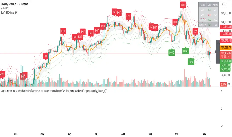
Ben's BTC Macro Fair Value OscillatorBen's BTC Macro Fair Value Oscillator
Overview
The **BTC Macro Fair Value Oscillator** is a non-crypto fair value framework that uses macro asset relationships (equities, dollar, gold) to estimate Bitcoin's "macro-driven fair value" and identify mean-reversion opportunities.
"Is BTC cheap or expensive right now?" on the 4 Hour Timeframe ONLY
### Key Features
✅ **Macro-driven**: Uses QQQ, DXY, XAUUSD instead of on-chain or crypto metrics
✅ **Dynamic weighting**: Assets weighted by rolling correlation strength
✅ **Mean-reversion signals**: Identifies when BTC is cheap/expensive vs macro
✅ **Validated parameters**: Optimized through 5-year backtest (Sharpe 6.7-9.9)
✅ **Visual transparency**: Live correlation panel, fair value bands, statistics
✅ **Non-repainting**: All calculations use confirmed historical data only
### What This Indicator Does
- Builds a **synthetic macro composite** from traditional assets
- Runs a **rolling regression** to predict BTC price from macro
- Calculates **deviation z-score** (how far BTC is from macro fair value)
- Generates **entry signals** when BTC is extremely cheap vs macro (dev < -2)
- Generates **exit signals** when BTC returns to fair value (dev > 0)
### What This Indicator Is NOT
❌ Not a high-frequency trading system (sparse signals by design)
❌ Not optimized for absolute returns (optimized for Sharpe ratio)
❌ Not suitable as standalone trading system (best as overlay/confirmation)
❌ Not predictive of short-term price movements (mean-reversion timeframe: days to weeks)
---
## Core Concept
### The Premise
Bitcoin doesn't trade in a vacuum. It's influenced by:
- **Risk appetite** (equities: QQQ, SPX)
- **Dollar strength** (DXY - inverse to risk assets)
- **Safe haven flows** (Gold: XAUUSD)
When macro conditions are "good for BTC" (risk-on, weak dollar, strong equities), BTC should trade higher. When macro conditions turn against it, BTC should trade lower.
### The Innovation
Instead of looking at BTC in isolation, this indicator:
1. **Measures how strongly** BTC currently correlates with each macro asset
2. **Builds a weighted composite** of those macro returns (the "D" driver)
3. **Regresses BTC price on D** to estimate "macro fair value"
4. **Tracks the deviation** between actual price and fair value
5. **Signals mean reversion** when deviation becomes extreme
### The Edge
The validated edge comes from:
- **Extreme deviations predict future returns** (dev < -2 → +1.67% over 12 bars)
- **Monotonic relationship** (more negative dev → higher forward returns)
- **Works out-of-sample** (test Sharpe +83-87% better than training)
- **Low correlation with buy & hold** (provides diversification value)
---
## Methodology
### Step 1: Macro Composite Driver D(t)
The indicator builds a weighted composite of macro asset returns:
**Process:**
1. Calculate **log returns** for BTC and each macro reference (QQQ, DXY, XAUUSD)
2. Compute **rolling correlation** between BTC and each reference over `corrLen` bars
3. **Weight each asset** by `|correlation|` if above `minCorrAbs` threshold, else 0
4. **Sign-adjust** weights (+1 for positive corr, -1 for negative) to handle inverse relationships
5. **Z-score normalize** each reference's returns over `fvWindow`
6. **Composite D(t)** = weighted sum of sign-adjusted z-scores
**Formula:**
```
For each reference i:
corr_i = correlation(BTC_returns, ref_i_returns, corrLen)
weight_i = |corr_i| if |corr_i| >= minCorrAbs else 0
sign_i = +1 if corr_i >= 0 else -1
z_i = (ref_i_returns - mean) / std
contrib_i = sign_i * z_i * weight_i
D(t) = sum(contrib_i) / sum(weight_i)
```
**Key Insight:** D(t) represents "how good macro conditions are for BTC right now" in a normalized, correlation-weighted way.
---
### Step 2: Fair Value Regression
Uses rolling linear regression to predict BTC price from D(t):
**Model:**
```
BTC_price(t) = α + β * D(t)
```
**Calculation (Pine Script approach):**
```
corr_CD = correlation(BTC_price, D, fvWindow)
sd_price = stdev(BTC_price, fvWindow)
sd_D = stdev(D, fvWindow)
cov = corr_CD * sd_price * sd_D
var_D = variance(D, fvWindow)
β = cov / var_D
α = mean(BTC_price) - β * mean(D)
fair_value(t) = α + β * D(t)
```
**Result:** A time-varying "macro fair value" line that adapts as correlations change.
---
### Step 3: Deviation Oscillator
Measures how far BTC price has deviated from fair value:
**Calculation:**
```
residual(t) = BTC_price(t) - fair_value(t)
residual_std = stdev(residual, normWindow)
deviation(t) = residual(t) / residual_std
```
**Interpretation:**
- `dev = 0` → BTC at fair value
- `dev = -2` → BTC is 2 standard deviations **cheap** vs macro
- `dev = +2` → BTC is 2 standard deviations **rich** vs macro
---
### Step 4: Signal Generation
**Long Entry:** `dev` crosses below `-2.0` (BTC extremely cheap vs macro)
**Long Exit:** `dev` crosses above `0.0` (BTC returns to fair value)
**No shorting** in default config (risk management choice - crypto volatility)
---
## How It Works
### Visual Components
#### 1. Price Chart (Main Panel)
**Fair Value Line (Orange):**
- The estimated "macro-driven fair value" for BTC
- Calculated from rolling regression on macro composite
**Fair Value Bands:**
- **±1σ** (light): 68% confidence zone
- **±2σ** (medium): 95% confidence zone
- **±3σ** (dark, dots): 99.7% confidence zone
**Entry/Exit Markers:**
- **Green "LONG" label** below bar: Entry signal (dev < -2)
- **Red "EXIT" label** above bar: Exit signal (dev > 0)
#### 2. Deviation Oscillator (Separate Pane)
**Line plot:**
- Shows current deviation z-score
- **Green** when dev < -2 (cheap)
- **Red** when dev > +2 (rich)
- **Gray** when neutral
**Histogram:**
- Visual representation of deviation magnitude
- Green bars = negative deviation (cheap)
- Red bars = positive deviation (rich)
**Threshold lines:**
- **Green dashed at -2.0**: Entry threshold
- **Red dashed at 0.0**: Exit threshold
- **Gray solid at 0**: Fair value line
#### 3. Correlation Panel (Top-Right)
Shows live correlation and weighting for each macro asset:
| Asset | Corr | Weight |
|-------|------|--------|
| QQQ | +0.45 | 0.45 |
| DXY | -0.32 | 0.32 |
| XAUUSD | +0.15 | 0.00 |
| Avg \|Corr\| | 0.31 | 0.77 |
**Reading:**
- **Corr**: Current rolling correlation with BTC (-1 to +1)
- **Weight**: How much this asset contributes to fair value (0 = excluded)
- **Avg |Corr|**: Average correlation strength (should be > 0.2 for reliable signals)
**Colors:**
- Green/Red corr = positive/negative correlation
- White weight = asset included, Gray = excluded (below minCorrAbs)
#### 4. Statistics Label (Bottom-Right)
```
━━━ BTC Macro FV ━━━
Dev: -2.34
Price: $103,192
FV: $110,500
Status: CHEAP ⬇
β: 103.52
```
**Fields:**
- **Dev**: Current deviation z-score
- **Price**: Current BTC close price
- **FV**: Current macro fair value estimate
- **Status**: CHEAP (< -2), RICH (> +2), or FAIR
- **β**: Current regression beta (sensitivity to macro)
---
## Installation & Setup
### TradingView Setup
1. Open TradingView and navigate to any **BTC chart** (BTCUSD, BTCUSDT, etc.)
2. Open **Pine Editor** (bottom panel)
3. Click **"+ New"** → **"Blank indicator"**
4. **Delete** all default code
5. **Copy** the entire Pine Script from `GHPT_optimized.pine`
6. **Paste** into the editor
7. Click **"Save"** and name it "BTC Macro Fair Value Oscillator"
8. Click **"Add to Chart"**
### Recommended Chart Settings
**Timeframe:** 4h (validated timeframe)
**Chart Type:** Candlestick or Heikin Ashi
**Overlay:** Yes (indicator plots on price chart + separate pane)
**Alternative Timeframes:**
- Daily: Works but slower signals
- 1h-2h: May work but not validated
- < 1h: Not recommended (too noisy)
### Symbol Requirements
**Primary:** BTC/USD or BTC/USDT on any exchange
**Macro References:** Automatically fetched
- QQQ (Nasdaq 100 ETF)
- DXY (US Dollar Index)
- XAUUSD (Gold spot)
**Data Requirements:**
- At least **90 bars** of history (warmup period)
- Premium TradingView recommended for full historical data
---
## Reading the Indicator
### Identifying Signals
#### Strong Long Signal (High Conviction)
- ✅ Deviation < -2.0 (extreme undervaluation)
- ✅ Avg |Corr| > 0.3 (strong macro relationships)
- ✅ Price touching or below -2σ band
- ✅ "LONG" label appears below bar
**Interpretation:** BTC is extremely cheap relative to macro conditions. Historical data shows +1.67% average return over next 12 bars (48 hours at 4h timeframe).
#### Moderate Long Signal (Lower Conviction)
- ⚠️ Deviation between -1.5 and -2.0
- ⚠️ Avg |Corr| between 0.2-0.3
- ⚠️ Price approaching -2σ band
**Interpretation:** BTC is cheap but not extreme. Consider as confirmation for other signals.
#### Exit Signal
- 🔴 Deviation crosses above 0 (returns to fair value)
- 🔴 "EXIT" label appears above bar
**Interpretation:** Mean reversion complete. Close long positions.
#### Strong Short/Avoid Signal
- 🔴 Deviation > +2.0 (extreme overvaluation)
- 🔴 Avg |Corr| > 0.3
- 🔴 Price touching or above +2σ band
**Interpretation:** BTC is expensive vs macro. Historical data shows -1.79% average return over next 12 bars. Consider exiting longs or reducing exposure.
### Regime Detection
**Strong Regime (Reliable Signals):**
- Avg |Corr| > 0.3
- Multiple assets weighted > 0
- Fair value line tracking price reasonably well
**Weak Regime (Unreliable Signals):**
- Avg |Corr| < 0.2
- Most weights = 0 (grayed out)
- Fair value line diverging wildly from price
- **Action:** Ignore signals until correlations strengthen
Weis Wave Volume MTF 🎯 Indicator Name
Weis Wave Volume (Multi‑Timeframe) — adapted from the original “Weis Wave Volume by LazyBear.”
This version adds multi‑timeframe (MTF) readings, configurable colors, font size, and screen position for clear dashboard‑style display.
🧠 Concept Background — What is Weis Wave Volume (WWV)?
The Weis Wave Volume indicator originates from Wyckoff and David Weis’ techniques.
Its purpose is to link price movement “waves” with the amount of traded volume to reveal how strong or weak each wave is.
Instead of showing bars one by one, WWV accumulates the total volume while price keeps moving in the same direction.
When price direction changes (up → down or down → up), it:
Finishes the previous wave volume total.
Starts a new wave and begins accumulating again.
Those wave volumes help traders see:
Effort vs Result: Big volume with small price move ⇒ absorption; low volume with big move ⇒ weak participation.
Trend confirmation or exhaustion: High volume waves in trend direction strengthen it, while low‑volume waves hint exhaustion.
⚙️ How this Script Works
Trend & Wave Detection
Compares close with the previous bar to determine up or down movement (mov).
Detects trend reversals (when mov direction changes).
Builds “waves,” each representing a continuous run of bars in one direction.
Volume Accumulation
While price keeps the same direction, the script adds each bar’s volume to the running total (vol).
When direction flips, it resets that total and starts a new wave.
Multi‑Timeframe Computation
Calculates these wave volumes on three timeframes at once, chosen dynamically:
Active Chart Timeframe Displays WWV for:
1 min 1 min
5 min 5 min
15 min 15 min
Any other Chart TF
It uses request.security() to pull each timeframe’s latest WWV value and current wave direction.
Visual Output
Instead of plotting histogram bars, it shows a table with three numeric values:
WWV (1): 25.3 M | (15): 312 M | (240): 2.46 B
Each value is color‑coded:
user‑selected Uptrend Color when price wave = up
user‑selected Downtrend Color when wave = down
You can position this small table in any corner/center (top / bottom × left / center / right).
Font size is user‑adjustable (Tiny → Huge).
📈 How Traders Use It
Quickly gauge buying vs selling effort across multiple horizons.
Compare short‑term wave volume to higher‑timeframe waves to spot:
Alignment → all up and big volumes = strong trend
Divergence → small or opposite‑colored higher‑TF wave = potential reversal or pause
Combine with Wyckoff, VSA, or standard trend analysis to judge if a breakout or pullback has real participation.
🧩 Key Features of This Version
Feature Description
Multi‑Timeframe Panel Displays WWV values for 3 selected TFs at once
Dynamic TF Mapping Auto‑adjusts which TFs to use based on chart
Up/Down Color Coding Customizable colors for wave direction
Adjustable Font and Placement Set font size (Tiny→Huge) and screen corner/center
No Histograms Keeps chart clean; acts as a compact WWV dashboard

Candlestick StrengthThis indicator quantifies the “energy” of each candlestick by combining its height (high–low span), trading volume, and internal structure (body vs. wick proportions). It provides a numeric measure of how strongly each candle contributes to market momentum, allowing traders to distinguish meaningful price action from indecision or noise.
Concept
Every candlestick represents a short-term contest between buyers and sellers. Large candles with significant volume indicate strong market participation, while small or low-volume candles suggest hesitation or absorption. Candlestick Strength captures this by calculating a normalized measure of each candle’s energy relative to recent activity, making it comparable across different market conditions and timeframes.
The indicator also analyzes the candle’s internal structure:
The body reflects net directional movement.
The wicks represent back-and-forth price traversal within the candle. Because wick movement does not fully contribute to directional momentum, it is weighted at half the body’s contribution. This ensures the indicator emphasizes sustained directional pressure while still acknowledging rejection or absorption.
Interpretation
High values indicate candles with energy above recent averages — suggesting expanding momentum and strong directional intent.
Average values reflect typical candle activity, representing neutral or steady market behavior.
Low values suggest weak candles — either the market is pausing, consolidating, or momentum is fading.
The outputs are displayed as a symmetric histogram: bullish candle energy is shown in green above zero, bearish energy in red below zero, with ±1 reference lines marking the normalized average energy level.
Usage
Combine with trend analysis, swing highs/lows, or volume-weighted averages to validate breakouts or trend continuation.
Monitor for divergence between price movement and candle energy to identify exhaustion, absorption, or potential reversals.
Filter out false momentum signals caused by narrow-range or low-volume candles.
Adaptable across timeframes: normalized energy allows comparison between small and large timeframe candles.

Velocity Pressure Index | AlphaNattVelocity Pressure Index (VPI) | AlphaNatt
A sophisticated momentum oscillator that combines price velocity analysis with volume pressure dynamics to identify high-probability trading opportunities.
📊 KEY FEATURES
Dual Analysis System: Merges price velocity measurement with volume pressure analysis for comprehensive market momentum assessment
Dynamic Normalization: Automatically scales values between -100 and +100 for consistent readings across all market conditions
Adaptive Zones: Self-adjusting overbought/oversold levels based on recent price history
Multi-Layer Confirmation: Combines momentum, acceleration, and crossover signals for robust trade identification
Volume-Weighted Pressure: Differentiates between bullish and bearish volume to gauge true market sentiment
📈 HOW IT WORKS
The VPI calculates price velocity using linear regression of price changes, then weights this velocity by the difference between bullish and bearish volume pressure. This creates a momentum reading that accounts for both price movement speed and the volume conviction behind it.
Signal Generation:
Price velocity is measured over the specified period
Volume is separated into bullish (close > open) and bearish (close < open) pressure
Velocity is amplified or dampened based on volume pressure differential
The resulting index is normalized to oscillate between -100 and +100
A signal line smooths the oscillator for crossover detection
🎯 TRADING SIGNALS
Long Signals (Cyan #00F1FF):
Strong Bull: VPI > Signal with positive momentum and acceleration
Crossover Bull: VPI crosses above signal while above oversold zone
Divergence: Price makes lower low while VPI makes higher low
Short Signals (Magenta #FF019A):
Strong Bear: VPI < Signal with negative momentum and deceleration
Crossover Bear: VPI crosses below signal while below overbought zone
Divergence: Price makes higher high while VPI makes lower high
⚙️ CUSTOMIZABLE PARAMETERS
Velocity Settings:
Velocity Period (14): Lookback for price velocity calculation
Pressure Period (21): Volume analysis window
Smoothing Factor (3): Final oscillator smoothing
Signal Configuration:
Signal Type: Choose between SMA, EMA, or DEMA
Signal Length (9): Signal line smoothing period
Normalization Period (50): Range calculation window
Dynamic Zones:
Zone Lookback (100): Period for adaptive overbought/oversold calculation
Percentiles: 80th/20th percentiles for dynamic zones
📐 VISUAL COMPONENTS
Main Oscillator: Color-coded line showing current momentum state
Signal Line: White line for crossover detection
Momentum Histogram: Shows velocity differential at 50% scale
Dynamic Zones: Self-adjusting overbought/oversold bands
Extreme Levels: ±50 dotted lines marking extreme conditions
Background Shading: Subtle highlighting of overbought/oversold regions
💡 USAGE TIPS
Trend Trading: Use strong bull/bear signals in trending markets for continuation entries
Range Trading: Focus on crossovers near extreme zones for reversal trades
Divergence Trading: Watch for price/oscillator divergences at market extremes
Multi-Timeframe: Combine with higher timeframe VPI for directional bias
Volume Confirmation: Stronger signals occur with aligned volume pressure
⚠️ BEST PRACTICES
The VPI works best in liquid markets with reliable volume data. For optimal results, combine with price action analysis and use appropriate risk management. The indicator is most effective during trending conditions but can identify reversals when divergences occur at extremes.
🔔 ALERTS AVAILABLE
VPI Long/Short Signals
Bullish/Bearish Crossovers
Extreme Overbought/Oversold Conditions
Version 6 | Pine Script™ | © AlphaNatt

5/15-Min-ORB-Trend-Finder-WiPIndicator Features:
> "Open" flag for each market day.
> Toggleable 5-min and 15-min High/Low markings.
> Horizontal support (red) and resistance (blue) lines.
> EMA-based trend line: green for long/buy, purple for short/sell.
> Recommended to use with my other indicator: Buy-or-Sell-WiP.
Strategy:
> Use with 1-min chart with 5-min High/Low or 5-min chart with 15-min High/Low
> After a breakout, wait for confirmation before placing a trade, which is:
- Two confirming candles (green for long/buy, red for short/sell)
and
- Buy-or-Sell-WiP histogram: green for long/buy, red for short/sell

Composite Momentum System⚙️ Composite Momentum System — RSI + CCI + Momentum + MFI + (DI·ADX) × MACD² (4-Color Smoothed Signal)
This advanced indicator fuses multiple momentum, volume, and trend components into one unified oscillator, dynamically visualized around a zero line. It helps traders identify powerful directional moves, trend reversals, and momentum exhaustion far earlier than traditional MACD or RSI alone.
🧩 Core Formula
Composite = ((RSI + CCI + Momentum + MFI) + (((DI− × −1) + DI+) × ADX)) × (MACD²)
RSI – captures relative strength and short-term momentum
CCI – measures deviation from price mean (volatility & cycles)
Momentum – shows raw velocity of price change
MFI – volume-weighted momentum, adds money flow confirmation
DI / ADX – directional strength and market trend intensity
MACD² – amplifies strong momentum moves and filters weak noise
🌈 Visual Design & Features
Zero-Centered Histogram:
Green = Bullish momentum, Red = Bearish momentum
MACD Signal Line (4 Colors):
🟢 Positive & Rising → strong up momentum
🟡 Positive & Falling → weakening uptrend
🔴 Negative & Falling → strong downtrend
🟠 Negative & Rising → possible bearish fade or reversal
Adjustable Signal Smoothing:
Choose MA type (SMA, EMA, RMA, WMA, VWMA) and custom smoothing length for cleaner visualization.
ATR Normalization:
Optional setting to keep MACD and composite values consistent across instruments.
Centering Options:
RSI and MFI can be centered (−50/+50) to balance oscillation around zero.
🎯 How to Use
Above 0: Bullish composite energy → favor long setups.
Below 0: Bearish composite energy → favor short setups.
Signal line color changes highlight momentum acceleration or slowdown.
Crosses through zero often precede major shifts or breakout moments.
⚡ Best Practice
Use this indicator as a momentum strength filter in confluence with price action or volume patterns.
Combine it with VWAP, higher-timeframe trend, or support/resistance zones for high-probability entries.
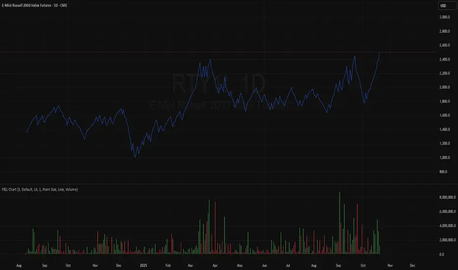
TASC 2025.11 The Points and Line Chart█ OVERVIEW
This script implements the Points and Line Chart described by Mohamed Ashraf Mahfouz and Mohamed Meregy in the November 2025 edition of the TASC Traders' Tips , "Efficient Display of Irregular Time Series”. This novel chart type interprets regular time series chart data to create an irregular time series chart.
█ CONCEPTS
When formatting data for display on a price chart, there are two main categorizations of chart types: regular time series (RTS) and irregular time series (ITS).
RTS charts, such as a typical candlestick chart, collect data over a specified amount of time and display it at one point. A one-minute candle, for example, represents the entirety of price movements within the minute that it represents.
ITS charts display data only after certain conditions are met. Since they do not plot at a consistent time period, they are called “irregular”.
Typically, ITS charts, such as Point and Figure (P&F) and Renko charts, focus on price change, plotting only when a certain threshold of change occurs.
The Points and Line (P&L) chart operates similarly to a P&F chart, using price change to determine when to plot points. However, instead of plotting the price in points, the P&L chart (by default) plots the closing price from RTS data. In other words, the P&L chart plots its points at the actual RTS close, as opposed to (price) intervals based on point size. This approach creates an ITS while still maintaining a reference to the RTS data, allowing us to gain a better understanding of time while consolidating the chart into an ITS format.
█ USAGE
Because the P&L chart forms bars based on price action instead of time, it displays displays significantly more history than a typical RTS chart. With this view, we are able to more easily spot support and resistance levels, which we could use when looking to place trades.
In the chart below, we can see over 13 years of data consolidated into one single view.
To view specific chart details, hover over each point of the chart to see a list of information.
In addition to providing a compact view of price movement over larger periods, this new chart type helps make classic chart patterns easier to interpret. When considering breakouts, the closing price provides a clearer representation of the actual breakout, as opposed to point size plots which are limited.
Because P&L is a new charting type, this script still requires a standard RTS chart for proper calculations. However, the main price chart is not intended for interpretation alongside the P&L chart; users can hide the main price series to keep the chart clean.
█ DISPLAYS
This indicator creates two displays: the "Price Display" and the "Data Display".
With the "Price display" setting, users can choose between showing a line or OHLC candles for the P&L drawing. The line display shows the close price of the P&L chart. In the candle display, the close price remains the same, while the open, high, and low values depend on the price action between points.
With the "Data display" setting, users can enable the display of a histogram that shows either the total volume or days/bars between the points in the P&L chart. For example, a reading of 12 days would indicate that the time since the last point was 12 days.
Note: The "Days" setting actually shows the number of chart bars elapsed between P&L points. The displayed value represents days only if the chart uses the "1D" timeframe.
The "Overlay P&L on chart" input controls whether the P&L line or candles appear on the main chart pane or in a separate pane.
Users can deactivate either display by selecting "None" from the corresponding input.
Technical Note: Due to drawing limitations, this indicator has the following display limits:
The line display can show data to 10,000 P&L points.
The candle display and tooltips show data for up to 500 points.
The histograms show data for up to 3,333 points.
█ INPUTS
Reversal Amount: The number of points/steps required to determine a reversal.
Scale size Method: The method used to filter price movements. By default, the P&L chart uses the same scaling method as the P&F chart. Optionally, this scaling method can be changed to use ATR or Percent.
P&L Method: The prices to plot and use for filtering:
“Close” plots the closing price and uses it to determine movements.
“High/Low” uses the high price on upside moves and low price on downside moves.
"Point Size" uses the closing price for filtration, but locks the price to plot at point size intervals.
Ripster: DTR/ATR + SMA Div + RVOL🧭 Overview
The indicator combines three major analytical tools into one TradingView Pine v6 script — designed for clean, at-a-glance insight into range, divergence, and volume activity.
It shows:
DTR vs ATR Table – current Daily True Range compared to Average True Range.
SMA Price Divergence + EMA Signal – a histogram with color-coded momentum bands.
RVOL Table + Candle Coloring + Change Labels – relative-volume analysis with visual cues on the chart.
Short title: ripcombo
Runs on chart overlay (no separate pane).
📊 1. DTR vs ATR Table
Compares today’s price range (High-Low) to the average true range over a selectable length.
Supports multiple smoothing methods: EMA, RMA, SMA, WMA.
Table position and text size are configurable.
Color logic:
🟢 ≤ 70 % of ATR → low volatility
🟡 70–90 % → average
🔴 ≥ 90 % → expanded range
📈 2. SMA Divergence + EMA Signal
Computes fast (14 SMA) and slow (30 SMA) divergences of price.
Plots two histograms plus an EMA signal line of the slow divergence.
Visuals:
Columns shaded by transparency for clarity.
Rising EMA → lime line (up momentum).
Falling EMA → red line (down momentum).
Optional upper/lower bands and zero line provide quick overbought/oversold zones.
🔥 3. RVOL (Relative Volume)
Adds powerful volume-based context:
a. Table Display
Shows:
Candle Volume
RVOL (Now)
RVOL (Prev)
Δ RVOL (change Now − Prev)
Colors:
🔴 > 200 % (very high volume)
🟠 100–200 % (high volume)
🟡 < 100 % (normal/low volume)
Δ column is green ▲ for increase, red ▼ for decrease.
b. Candle Coloring (optional)
Colors price candles themselves by current RVOL threshold so high-volume candles visually stand out.
c. Last-Bar Label (optional)
Prints a compact label on the latest candle showing:
RVOL: ### % Δ: ▲/▼## %
so you can instantly see the current volume strength and how it changed from the previous bar.
⚙️ User Settings
All major elements are toggle-controlled:
Enable/disable ATR, Divergence, or RVOL sections.
Choose table positions (top/middle/bottom × left/center/right).
Select text sizes, smoothing types, color modes, and visual transparency.
Candle coloring + label visibility are optional.
🧠 At a Glance
Component Purpose Key Visuals
DTR vs ATR Measures volatility expansion One-cell colored table
SMA Divergence Detects price momentum shifts Columns + EMA line + bands
RVOL Analysis Highlights unusual trading volume Colored table + Δ column + candle colors + label
✅ Result
You get a single on-chart tool that:
Quantifies volatility, momentum, and volume context together.
Highlights strong activity days (ATR & RVOL) in color.
Shows whether current candle’s volume is rising or falling vs the previous.
Perfect for spotting breakouts, reversals, or exhaustion moves without switching indicators.
