ICT Master Suite [Trading IQ]Hello Traders!
We’re excited to introduce the ICT Master Suite by TradingIQ, a new tool designed to bring together several ICT concepts and strategies in one place.
The Purpose Behind the ICT Master Suite
There are a few challenges traders often face when using ICT-related indicators:
Many available indicators focus on one or two ICT methods, which can limit traders who apply a broader range of ICT related techniques on their charts.
There aren't many indicators for ICT strategy models, and we couldn't find ICT indicators that allow for testing the strategy models and setting alerts.
Many ICT related concepts exist in the public domain as indicators, not strategies! This makes it difficult to verify that the ICT concept has some utility in the market you're trading and if it's worth trading - it's difficult to know if it's working!
Some users might not have enough chart space to apply numerous ICT related indicators, which can be restrictive for those wanting to use multiple ICT techniques simultaneously.
The ICT Master Suite is designed to offer a comprehensive option for traders who want to apply a variety of ICT methods. By combining several ICT techniques and strategy models into one indicator, it helps users maximize their chart space while accessing multiple tools in a single slot.
Additionally, the ICT Master Suite was developed as a strategy . This means users can backtest various ICT strategy models - including deep backtesting. A primary goal of this indicator is to let traders decide for themselves what markets to trade ICT concepts in and give them the capability to figure out if the strategy models are worth trading!
What Makes the ICT Master Suite Different
There are many ICT-related indicators available on TradingView, each offering valuable insights. What the ICT Master Suite aims to do is bring together a wider selection of these techniques into one tool. This includes both key ICT methods and strategy models, allowing traders to test and activate strategies all within one indicator.
Features
The ICT Master Suite offers:
Multiple ICT strategy models, including the 2022 Strategy Model and Unicorn Model, which can be built, tested, and used for live trading.
Calculation and display of key price areas like Breaker Blocks, Rejection Blocks, Order Blocks, Fair Value Gaps, Equal Levels, and more.
The ability to set alerts based on these ICT strategies and key price areas.
A comprehensive, yet practical, all-inclusive ICT indicator for traders.
Customizable Timeframe - Calculate ICT concepts on off-chart timeframes
Unicorn Strategy Model
2022 Strategy Model
Liquidity Raid Strategy Model
OTE (Optimal Trade Entry) Strategy Model
Silver Bullet Strategy Model
Order blocks
Breaker blocks
Rejection blocks
FVG
Strong highs and lows
Displacements
Liquidity sweeps
Power of 3
ICT Macros
HTF previous bar high and low
Break of Structure indications
Market Structure Shift indications
Equal highs and lows
Swings highs and swing lows
Fibonacci TPs and SLs
Swing level TPs and SLs
Previous day high and low TPs and SLs
And much more! An ongoing project!
How To Use
Many traders will already be familiar with the ICT related concepts listed above, and will find using the ICT Master Suite quite intuitive!
Despite this, let's go over the features of the tool in-depth and how to use the tool!
The image above shows the ICT Master Suite with almost all techniques activated.
ICT 2022 Strategy Model
The ICT Master suite provides the ability to test, set alerts for, and live trade the ICT 2022 Strategy Model.
The image above shows an example of a long position being entered following a complete setup for the 2022 ICT model.
A liquidity sweep occurs prior to an upside breakout. During the upside breakout the model looks for the FVG that is nearest 50% of the setup range. A limit order is placed at this FVG for entry.
The target entry percentage for the range is customizable in the settings. For instance, you can select to enter at an FVG nearest 33% of the range, 20%, 66%, etc.
The profit target for the model generally uses the highest high of the range (100%) for longs and the lowest low of the range (100%) for shorts. Stop losses are generally set at 0% of the range.
The image above shows the short model in action!
Whether you decide to follow the 2022 model diligently or not, you can still set alerts when the entry condition is met.
ICT Unicorn Model
The image above shows an example of a long position being entered following a complete setup for the ICT Unicorn model.
A lower swing low followed by a higher swing high precedes the overlap of an FVG and breaker block formed during the sequence.
During the upside breakout the model looks for an FVG and breaker block that formed during the sequence and overlap each other. A limit order is placed at the nearest overlap point to current price.
The profit target for this example trade is set at the swing high and the stop loss at the swing low. However, both the profit target and stop loss for this model are configurable in the settings.
For Longs, the selectable profit targets are:
Swing High
Fib -0.5
Fib -1
Fib -2
For Longs, the selectable stop losses are:
Swing Low
Bottom of FVG or breaker block
The image above shows the short version of the Unicorn Model in action!
For Shorts, the selectable profit targets are:
Swing Low
Fib -0.5
Fib -1
Fib -2
For Shorts, the selectable stop losses are:
Swing High
Top of FVG or breaker block
The image above shows the profit target and stop loss options in the settings for the Unicorn Model.
Optimal Trade Entry (OTE) Model
The image above shows an example of a long position being entered following a complete setup for the OTE model.
Price retraces either 0.62, 0.705, or 0.79 of an upside move and a trade is entered.
The profit target for this example trade is set at the -0.5 fib level. This is also adjustable in the settings.
For Longs, the selectable profit targets are:
Swing High
Fib -0.5
Fib -1
Fib -2
The image above shows the short version of the OTE Model in action!
For Shorts, the selectable profit targets are:
Swing Low
Fib -0.5
Fib -1
Fib -2
Liquidity Raid Model
The image above shows an example of a long position being entered following a complete setup for the Liquidity Raid Modell.
The user must define the session in the settings (for this example it is 13:30-16:00 NY time).
During the session, the indicator will calculate the session high and session low. Following a “raid” of either the session high or session low (after the session has completed) the script will look for an entry at a recently formed breaker block.
If the session high is raided the script will look for short entries at a bearish breaker block. If the session low is raided the script will look for long entries at a bullish breaker block.
For Longs, the profit target options are:
Swing high
User inputted Lib level
For Longs, the stop loss options are:
Swing low
User inputted Lib level
Breaker block bottom
The image above shows the short version of the Liquidity Raid Model in action!
For Shorts, the profit target options are:
Swing Low
User inputted Lib level
For Shorts, the stop loss options are:
Swing High
User inputted Lib level
Breaker block top
Silver Bullet Model
The image above shows an example of a long position being entered following a complete setup for the Silver Bullet Modell.
During the session, the indicator will determine the higher timeframe bias. If the higher timeframe bias is bullish the strategy will look to enter long at an FVG that forms during the session. If the higher timeframe bias is bearish the indicator will look to enter short at an FVG that forms during the session.
For Longs, the profit target options are:
Nearest Swing High Above Entry
Previous Day High
For Longs, the stop loss options are:
Nearest Swing Low
Previous Day Low
The image above shows the short version of the Silver Bullet Model in action!
For Shorts, the profit target options are:
Nearest Swing Low Below Entry
Previous Day Low
For Shorts, the stop loss options are:
Nearest Swing High
Previous Day High
Order blocks
The image above shows indicator identifying and labeling order blocks.
The color of the order blocks, and how many should be shown, are configurable in the settings!
Breaker Blocks
The image above shows indicator identifying and labeling order blocks.
The color of the breaker blocks, and how many should be shown, are configurable in the settings!
Rejection Blocks
The image above shows indicator identifying and labeling rejection blocks.
The color of the rejection blocks, and how many should be shown, are configurable in the settings!
Fair Value Gaps
The image above shows indicator identifying and labeling fair value gaps.
The color of the fair value gaps, and how many should be shown, are configurable in the settings!
Additionally, you can select to only show fair values gaps that form after a liquidity sweep. Doing so reduces "noisy" FVGs and focuses on identifying FVGs that form after a significant trading event.
The image above shows the feature enabled. A fair value gap that occurred after a liquidity sweep is shown.
Market Structure
The image above shows the ICT Master Suite calculating market structure shots and break of structures!
The color of MSS and BoS, and whether they should be displayed, are configurable in the settings.
Displacements
The images above show indicator identifying and labeling displacements.
The color of the displacements, and how many should be shown, are configurable in the settings!
Equal Price Points
The image above shows the indicator identifying and labeling equal highs and equal lows.
The color of the equal levels, and how many should be shown, are configurable in the settings!
Previous Custom TF High/Low
The image above shows the ICT Master Suite calculating the high and low price for a user-defined timeframe. In this case the previous day’s high and low are calculated.
To illustrate the customizable timeframe function, the image above shows the indicator calculating the previous 4 hour high and low.
Liquidity Sweeps
The image above shows the indicator identifying a liquidity sweep prior to an upside breakout.
The image above shows the indicator identifying a liquidity sweep prior to a downside breakout.
The color and aggressiveness of liquidity sweep identification are adjustable in the settings!
Power Of Three
The image above shows the indicator calculating Po3 for two user-defined higher timeframes!
Macros
The image above shows the ICT Master Suite identifying the ICT macros!
ICT Macros are only displayable on the 5 minute timeframe or less.
Strategy Performance Table
In addition to a full-fledged TradingView backtest for any of the ICT strategy models the indicator offers, a quick-and-easy strategy table exists for the indicator!
The image above shows the strategy performance table in action.
Keep in mind that, because the ICT Master Suite is a strategy script, you can perform fully automatic backtests, deep backtests, easily add commission and portfolio balance and look at pertinent metrics for the ICT strategies you are testing!
Lite Mode
Traders who want the cleanest chart possible can toggle on “Lite Mode”!
In Lite Mode, any neon or “glow” like effects are removed and key levels are marked as strict border boxes. You can also select to remove box borders if that’s what you prefer!
Settings Used For Backtest
For the displayed backtest, a starting balance of $1000 USD was used. A commission of 0.02%, slippage of 2 ticks, a verify price for limit orders of 2 ticks, and 5% of capital investment per order.
A commission of 0.02% was used due to the backtested asset being a perpetual future contract for a crypto currency. The highest commission (lowest-tier VIP) for maker orders on many exchanges is 0.02%. All entered positions take place as maker orders and so do profit target exits. Stop orders exist as stop-market orders.
A slippage of 2 ticks was used to simulate more realistic stop-market orders. A verify limit order settings of 2 ticks was also used. Even though BTCUSDT.P on Binance is liquid, we just want the backtest to be on the safe side. Additionally, the backtest traded 100+ trades over the period. The higher the sample size the better; however, this example test can serve as a starting point for traders interested in ICT concepts.
Community Assistance And Feedback
Given the complexity and idiosyncratic applications of ICT concepts amongst its proponents, the ICT Master Suite’s built-in strategies and level identification methods might not align with everyone's interpretation.
That said, the best we can do is precisely define ICT strategy rules and concepts to a repeatable process, test, and apply them! Whether or not an ICT strategy is trading precisely how you would trade it, seeing the model in action, taking trades, and with performance statistics is immensely helpful in assessing predictive utility.
If you think we missed something, you notice a bug, have an idea for strategy model improvement, please let us know! The ICT Master Suite is an ongoing project that will, ideally, be shaped by the community.
A big thank you to the @PineCoders for their Time Library!
Thank you!
Cari skrip untuk "high low"

AlgoBuilder [Trend-Following] | FractalystWhat's the strategy's purpose and functionality?
This strategy is designed for both traders and investors looking to rely on and trade based on historical and backtested data using automation. The main goal is to build profitable trend-following strategies that outperform the underlying asset in terms of returns while minimizing drawdown. For example, as for a benchmark, if the S&P 500 (SPX) has achieved an estimated 10% annual return with a maximum drawdown of -57% over the past 20 years, using this strategy with different entry and exit techniques, users can potentially seek ways to achieve a higher Compound Annual Growth Rate (CAGR) while maintaining a lower maximum drawdown.
Although the strategy can be applied to all markets and timeframes, it is most effective on stocks, indices, future markets, cryptocurrencies, and commodities and JPY currency pairs given their trending behaviors.
In trending market conditions, the strategy employs a combination of moving averages and diverse entry models to identify and capitalize on upward market movements. It integrates market structure-based trailing stop-loss mechanisms across different timeframes and provides exit techniques, including percentage-based and risk-reward (RR) based take profit levels.
Additionally, the strategy has also a feature that includes a built-in probability and sentiment function for traders who want to implement probabilities and market sentiment right into their trading strategies.
Performance summary, weekly, and monthly tables enable quick visualization of performance metrics like net profit, maximum drawdown, compound annual growth rate (CAGR), profit factor, average trade, average risk-reward ratio (RR), and more. This aids optimization to meet specific goals and risk tolerance levels effectively.
-----
How does the strategy perform for both investors and traders?
The strategy has two main modes, tailored for different market participants: Traders and Investors.
Trading:
1. Trading (1x):
- Designed for traders looking to capitalize on bullish trending markets.
- Utilizes a percentage risk per trade to manage risk and optimize returns.
- Suitable for active trading with a focus on trend-following and risk management.
- (1x) This mode ensures no stacking of positions, allowing for only one running position or trade at a time.
◓: Mode | %: Risk percentage per trade
2. Trading (2x):
Similar to the 1x mode but allows for two pyramiding entries.
This approach enables traders to increase their position size as the trade moves in their favor, potentially enhancing profits during strong bullish trends.
◓: Mode | %: Risk percentage per trade
3. Investing:
- Geared towards investors who aim to capitalize on bullish trending markets without using leverage while mitigating the asset's maximum drawdown.
- Utilizes 100% of the equity to buy, hold, and manage the asset.
- Focuses on long-term growth and capital appreciation by fully investing in the asset during bullish conditions.
- ◓: Mode | %: Risk not applied (In investing mode, the strategy uses 100% of equity to buy the asset)
-----
What's the purpose of using moving averages in this strategy? What are the underlying calculations?
Using moving averages is a widely-used technique to trade with the trend.
The main purpose of using moving averages in this strategy is to filter out bearish price action and to only take trades when the price is trading ABOVE specified moving averages.
The script uses different types of moving averages with user-adjustable timeframes and periods/lengths, allowing traders to try out different variations to maximize strategy performance and minimize drawdowns.
By applying these calculations, the strategy effectively identifies bullish trends and avoids market conditions that are not conducive to profitable trades.
The MA filter allows traders to choose whether they want a specific moving average above or below another one as their entry condition.
This comparison filter can be turned on (>/<) or off.
For example, you can set the filter so that MA#1 > MA#2, meaning the first moving average must be above the second one before the script looks for entry conditions. This adds an extra layer of trend confirmation, ensuring that trades are only taken in more favorable market conditions.
MA #1: Fast MA | MA #2: Medium MA | MA #3: Slow MA
⍺: MA Period | Σ: MA Timeframe
-----
What entry modes are used in this strategy? What are the underlying calculations?
The strategy by default uses two different techniques for the entry criteria with user-adjustable left and right bars: Breakout and Fractal.
1. Breakout Entries :
- The strategy looks for pivot high points with a default period of 3.
- It stores the most recent high level in a variable.
- When the price crosses above this most recent level, the strategy checks if all conditions are met and the bar is closed before taking the buy entry.
◧: Pivot high left bars period | ◨: Pivot high right bars period
2. Fractal Entries :
- The strategy looks for pivot low points with a default period of 3.
- When a pivot low is detected, the strategy checks if all conditions are met and the bar is closed before taking the buy entry.
◧: Pivot low left bars period | ◨: Pivot low right bars period
By utilizing these entry modes, the strategy aims to capitalize on bullish price movements while ensuring that the necessary conditions are met to validate the entry points.
-----
What type of stop-loss identification method are used in this strategy? What are the underlying calculations?
Initial Stop-Loss:
1. ATR Based:
The Average True Range (ATR) is a method used in technical analysis to measure volatility. It is not used to indicate the direction of price but to measure volatility, especially volatility caused by price gaps or limit moves.
Calculation:
- To calculate the ATR, the True Range (TR) first needs to be identified. The TR takes into account the most current period high/low range as well as the previous period close.
The True Range is the largest of the following:
- Current Period High minus Current Period Low
- Absolute Value of Current Period High minus Previous Period Close
- Absolute Value of Current Period Low minus Previous Period Close
- The ATR is then calculated as the moving average of the TR over a specified period. (The default period is 14).
Example - ATR (14) * 1.5
⍺: ATR period | Σ: ATR Multiplier
2. ADR Based:
The Average Day Range (ADR) is an indicator that measures the volatility of an asset by showing the average movement of the price between the high and the low over the last several days.
Calculation:
- To calculate the ADR for a particular day:
- Calculate the average of the high prices over a specified number of days.
- Calculate the average of the low prices over the same number of days.
- Find the difference between these average values.
- The default period for calculating the ADR is 14 days. A shorter period may introduce more noise, while a longer period may be slower to react to new market movements.
Example - ADR (14) * 1.5
⍺: ADR period | Σ: ADR Multiplier
Application in Strategy:
- The strategy calculates the current bar's ADR/ATR with a user-defined period.
- It then multiplies the ADR/ATR by a user-defined multiplier to determine the initial stop-loss level.
By using these methods, the strategy dynamically adjusts the initial stop-loss based on market volatility, helping to protect against adverse price movements while allowing for enough room for trades to develop.
Trailing Stop-Loss:
One of the key elements of this strategy is its ability to detec buyside and sellside liquidity levels across multiple timeframes to trail the stop-loss once the trade is in running profits.
By utilizing this approach, the strategy allows enough room for price to run.
There are two built-in trailing stop-loss (SL) options you can choose from while in a trade:
1. External Trailing Stop-Loss:
- Uses sell-side liquidity to trail your stop-loss, allowing price to consolidate before continuation. This method is less aggressive and provides more room for price fluctuations.
Example - External - Wick below the trailing SL - 12H trailing timeframe
⍺: Exit type | Σ: Trailing stop-loss timeframe
2. Internal Trailing Stop-Loss:
- Uses the most recent swing low with a period of 2 to trail your stop-loss. This method is more aggressive compared to the external trailing stop-loss, as it tightens the stop-loss closer to the current price action.
Example - Internal - Close below the trailing SL - 6H trailing timeframe
⍺: Exit type | Σ: Trailing stop-loss timeframe
Each market behaves differently across various timeframes, and it is essential to test different parameters and optimizations to find out which trailing stop-loss method gives you the desired results and performance.
-----
What type of break-even and take profit identification methods are used in this strategy? What are the underlying calculations?
For Break-Even:
- You can choose to set a break-even level at which your initial stop-loss moves to the entry price as soon as it hits, and your trailing stop-loss gets activated (if enabled).
- You can select either a percentage (%) or risk-to-reward (RR) based break-even, allowing you to set your break-even level as a percentage amount above the entry price or based on RR.
For TP1 (Take Profit 1):
- You can choose to set a take profit level at which your position gets fully closed or 50% if the TP2 boolean is enabled.
- Similar to break-even, you can select either a percentage (%) or risk-to-reward (RR) based take profit level, allowing you to set your TP1 level as a percentage amount above the entry price or based on RR.
For TP2 (Take Profit 2):
- You can choose to set a take profit level at which your position gets fully closed.
- As with break-even and TP1, you can select either a percentage (%) or risk-to-reward (RR) based take profit level, allowing you to set your TP2 level as a percentage amount above the entry price or based on RR.
The underlying calculations involve determining the price levels at which these actions are triggered. For break-even, it moves the initial stop-loss to the entry price and activate the trailing stop-loss once the break-even level is reached.
For TP1 and TP2, it's specifying the price levels at which the position is partially or fully closed based on the chosen method (percentage or RR) above the entry price.
These calculations are crucial for managing risk and optimizing profitability in the strategy.
⍺: BE/TP type (%/RR) | Σ: how many RR/% above the current price
-----
What's the ADR filter? What does it do? What are the underlying calculations?
The Average Day Range (ADR) measures the volatility of an asset by showing the average movement of the price between the high and the low over the last several days.
The period of the ADR filter used in this strategy is tied to the same period you've used for your initial stop-loss.
Users can define the minimum ADR they want to be met before the script looks for entry conditions.
ADR Bias Filter:
- Compares the current bar ADR with the ADR (Defined by user):
- If the current ADR is higher, it indicates that volatility has increased compared to ADR (DbU).(⬆)
- If the current ADR is lower, it indicates that volatility has decreased compared to ADR (DbU).(⬇)
Calculations:
1. Calculate ADR:
- Average the high prices over the specified period.
- Average the low prices over the same period.
- Find the difference between these average values in %.
2. Current ADR vs. ADR (DbU):
- Calculate the ADR for the current bar.
- Calculate the ADR (DbU).
- Compare the two values to determine if volatility has increased or decreased.
By using the ADR filter, the strategy ensures that trades are only taken in favorable market conditions where volatility meets the user's defined threshold, thus optimizing entry conditions and potentially improving the overall performance of the strategy.
>: Minimum required ADR for entry | %: Current ADR comparison to ADR of 14 days ago.
-----
What's the probability filter? What are the underlying calculations?
The probability filter is designed to enhance trade entries by using buyside liquidity and probability analysis to filter out unfavorable conditions.
This filter helps in identifying optimal entry points where the likelihood of a profitable trade is higher.
Calculations:
1. Understanding Swing highs and Swing Lows
Swing High: A Swing High is formed when there is a high with 2 lower highs to the left and right.
Swing Low: A Swing Low is formed when there is a low with 2 higher lows to the left and right.
2. Understanding the purpose and the underlying calculations behind Buyside, Sellside and Equilibrium levels.
3. Understanding probability calculations
1. Upon the formation of a new range, the script waits for the price to reach and tap into equilibrium or the 50% level. Status: "⏸" - Inactive
2. Once equilibrium is tapped into, the equilibrium status becomes activated and it waits for either liquidity side to be hit. Status: "▶" - Active
3. If the buyside liquidity is hit, the script adds to the count of successful buyside liquidity occurrences. Similarly, if the sellside is tapped, it records successful sellside liquidity occurrences.
5. Finally, the number of successful occurrences for each side is divided by the overall count individually to calculate the range probabilities.
Note: The calculations are performed independently for each directional range. A range is considered bearish if the previous breakout was through a sellside liquidity. Conversely, a range is considered bullish if the most recent breakout was through a buyside liquidity.
Example - BSL > 50%
-----
What's the sentiment Filter? What are the underlying calculations?
Sentiment filter aims to calculate the percentage level of bullish or bearish fluctuations within equally divided price sections, in the latest price range.
Calculations:
This filter calculates the current sentiment by identifying the highest swing high and the lowest swing low, then evenly dividing the distance between them into percentage amounts. If the price is above the 50% mark, it indicates bullishness, whereas if it's below 50%, it suggests bearishness.
Sentiment Bias Identification:
Bullish Bias: The current price is trading above the 50% daily range.
Bearish Bias: The current price is trading below the 50% daily range.
Example - Sentiment Enabled | Bullish degree above 50% | Bullish sentimental bias
>: Minimum required sentiment for entry | %: Current sentimental degree in a (Bullish/Bearish) sentimental bias
-----
What's the range length Filter? What are the underlying calculations?
The range length filter identifies the price distance between buyside and sellside liquidity levels in percentage terms. When enabled, the script only looks for entries when the minimum range length is met. This helps ensure that trades are taken in markets with sufficient price movement.
Calculations:
Range Length (%) = ( ( Buyside Level − Sellside Level ) / Current Price ) ×100
Range Bias Identification:
Bullish Bias: The current range price has broken above the previous external swing high.
Bearish Bias: The current range price has broken below the previous external swing low.
Example - Range length filter is enabled | Range must be above 5% | Price must be in a bearish range
>: Minimum required range length for entry | %: Current range length percentage in a (Bullish/Bearish) range
-----
What's the day filter Filter, what does it do?
The day filter allows users to customize the session time and choose the specific days they want to include in the strategy session. This helps traders tailor their strategies to particular trading sessions or days of the week when they believe the market conditions are more favorable for their trading style.
Customize Session Time:
Users can define the start and end times for the trading session.
This allows the strategy to only consider trades within the specified time window, focusing on periods of higher market activity or preferred trading hours.
Select Days:
Users can select which days of the week to include in the strategy.
This feature is useful for excluding days with historically lower volatility or unfavorable trading conditions (e.g., Mondays or Fridays).
Benefits:
Focus on Optimal Trading Periods:
By customizing session times and days, traders can focus on periods when the market is more likely to present profitable opportunities.
Avoid Unfavorable Conditions:
Excluding specific days or times can help avoid trading during periods of low liquidity or high unpredictability, such as major news events or holidays.
Increased Flexibility: The filter provides increased flexibility, allowing traders to adapt the strategy to their specific needs and preferences.
Example - Day filter | Session Filter
θ: Session time | Exchange time-zone
-----
What tables are available in this script?
Table Type:
- Summary: Provides a general overview, displaying key performance parameters such as Net Profit, Profit Factor, Max Drawdown, Average Trade, Closed Trades, Compound Annual Growth Rate (CAGR), MAR and more.
CAGR: It calculates the 'Compound Annual Growth Rate' first and last taken trades on your chart. The CAGR is a notional, annualized growth rate that assumes all profits are reinvested. It only takes into account the prices of the two end points — not drawdowns, so it does not calculate risk. It can be used as a yardstick to compare the performance of two strategies. Since it annualizes values, it requires a minimum 4H timeframe to display the CAGR value. annualizing returns over smaller periods of times doesn't produce very meaningful figures.
MAR: Measure of return adjusted for risk: CAGR divided by Max Drawdown. Indicates how comfortable the system might be to trade. Higher than 0.5 is ideal, 1.0 and above is very good, and anything above 3.0 should be considered suspicious and you need to make sure the total number of trades are high enough by running a Deep Backtest in strategy tester. (available for TradingView Premium users.)
Avg Trade: The sum of money gained or lost by the average trade generated by a strategy. Calculated by dividing the Net Profit by the overall number of closed trades. An important value since it must be large enough to cover the commission and slippage costs of trading the strategy and still bring a profit.
MaxDD: Displays the largest drawdown of losses, i.e., the maximum possible loss that the strategy could have incurred among all of the trades it has made. This value is calculated separately for every bar that the strategy spends with an open position.
Profit Factor: The amount of money a trading strategy made for every unit of money it lost (in the selected currency). This value is calculated by dividing gross profits by gross losses.
Avg RR: This is calculated by dividing the average winning trade by the average losing trade. This field is not a very meaningful value by itself because it does not take into account the ratio of the number of winning vs losing trades, and strategies can have different approaches to profitability. A strategy may trade at every possibility in order to capture many small profits, yet have an average losing trade greater than the average winning trade. The higher this value is, the better, but it should be considered together with the percentage of winning trades and the net profit.
Winrate: The percentage of winning trades generated by a strategy. Calculated by dividing the number of winning trades by the total number of closed trades generated by a strategy. Percent profitable is not a very reliable measure by itself. A strategy could have many small winning trades, making the percent profitable high with a small average winning trade, or a few big winning trades accounting for a low percent profitable and a big average winning trade. Most trend-following successful strategies have a percent profitability of 15-40% but are profitable due to risk management control.
BE Trades: Number of break-even trades, excluding commission/slippage.
Losing Trades: The total number of losing trades generated by the strategy.
Winning Trades: The total number of winning trades generated by the strategy.
Total Trades: Total number of taken traders visible your charts.
Net Profit: The overall profit or loss (in the selected currency) achieved by the trading strategy in the test period. The value is the sum of all values from the Profit column (on the List of Trades tab), taking into account the sign.
- Monthly: Displays performance data on a month-by-month basis, allowing users to analyze performance trends over each month.
- Weekly: Displays performance data on a week-by-week basis, helping users to understand weekly performance variations.
- OFF: Hides the performance table.
Labels:
- OFF: Hides labels in the performance table.
- PnL: Shows the profit and loss of each trade individually, providing detailed insights into the performance of each trade.
- Range: Shows the range length and Average Day Range (ADR), offering additional context about market conditions during each trade.
Profit Color:
- Allows users to set the color for representing profit in the performance table, helping to quickly distinguish profitable periods.
Loss Color:
- Allows users to set the color for representing loss in the performance table, helping to quickly identify loss-making periods.
These customizable tables provide traders with flexible and detailed performance analysis, aiding in better strategy evaluation and optimization.
-----
User-input styles and customizations:
To facilitate studying historical data, all conditions and rules can be applied to your charts. By plotting background colors on your charts, you'll be able to identify what worked and what didn't in certain market conditions.
Please note that all background colors in the style are disabled by default to enhance visualization.
-----
How to Use This Algobuilder to Create a Profitable Edge and System:
Choose Your Strategy mode:
- Decide whether you are creating an investing strategy or a trading strategy.
Select a Market:
- Choose a one-sided market such as stocks, indices, or cryptocurrencies.
Historical Data:
- Ensure the historical data covers at least 10 years of price action for robust backtesting.
Timeframe Selection:
- Choose the timeframe you are comfortable trading with. It is strongly recommended to use a timeframe above 15 minutes to minimize the impact of commissions on your profits.
Set Commission and Slippage:
- Properly set the commission and slippage in the strategy properties according to your broker or prop firm specifications.
Parameter Optimization:
- Use trial and error to test different parameters until you find the performance results you are looking for in the summary table or, preferably, through deep backtesting using the strategy tester.
Trade Count:
- Ensure the number of trades is 100 or more; the higher, the better for statistical significance.
Positive Average Trade:
- Make sure the average trade value is above zero.
(An important value since it must be large enough to cover the commission and slippage costs of trading the strategy and still bring a profit.)
Performance Metrics:
- Look for a high profit factor, MAR (Mar Ratio), CAGR (Compound Annual Growth Rate), and net profit with minimum drawdown. Ideally, aim for a drawdown under 20-30%, depending on your risk tolerance.
Refinement and Optimization:
- Try out different markets and timeframes.
- Continue working on refining your edge using the available filters and components to further optimize your strategy.
Automation:
- Once you’re confident in your strategy, you can use the automation section to connect the algorithm to your broker or prop firm.
- Trade a fully automated and backtested trading strategy, allowing for hands-free execution and management.
-----
What makes this strategy original?
1. Incorporating direct integration of probabilities into the strategy.
2. Leveraging market sentiment to construct a profitable approach.
3. Utilizing built-in market structure-based trailing stop-loss mechanisms across various timeframes.
4. Offering both investing and trading strategies, facilitating optimization from different perspectives.
5. Automation for efficient execution.
6. Providing a summary table for instant access to key parameters of the strategy.
-----
How to use automation?
For Traders:
1. Ensure the strategy parameters are properly set based on your optimized parameters.
2. Enter your PineConnector License ID in the designated field.
3. Specify the desired risk level.
4. Provide the Metatrader symbol.
5. Check for chart updates to ensure the automation table appears on the top right corner, displaying your License ID, risk, and symbol.
6. Set up an alert with the strategy selected as Condition and the Message as {{strategy.order.alert_message}}.
7. Activate the Webhook URL in the Notifications section, setting it as the official PineConnector webhook address.
8. Double-check all settings on PineConnector to ensure the connection is successful.
9. Create the alert for entry/exit automation.
For Investors:
1. Ensure the strategy parameters are properly set based on your optimized parameters.
2. Choose "Investing" in the user-input settings.
3. Create an alert with a specified name.
4. Customize the notifications tab to receive alerts via email.
5. Buying/selling alerts will be triggered instantly upon entry or exit order execution.
----
Strategy Properties
This script backtest is done on 4H COINBASE:BTCUSD , using the following backtesting properties:
Balance: $5000
Order Size: 10% of the equity
Risk % per trade: 1%
Commission: 0.04% (Default commission percentage according to TradingView competitions rules)
Slippage: 75 ticks
Pyramiding: 2
-----
Terms and Conditions | Disclaimer
Our charting tools are provided for informational and educational purposes only and should not be construed as financial, investment, or trading advice. They are not intended to forecast market movements or offer specific recommendations. Users should understand that past performance does not guarantee future results and should not base financial decisions solely on historical data.
Built-in components, features, and functionalities of our charting tools are the intellectual property of @Fractalyst Unauthorized use, reproduction, or distribution of these proprietary elements is prohibited.
By continuing to use our charting tools, the user acknowledges and accepts the Terms and Conditions outlined in this legal disclaimer and agrees to respect our intellectual property rights and comply with all applicable laws and regulations.

Reversal Point Dynamics - Machine Learning⇋ Reversal Point Dynamics - Machine Learning
RPD Machine Learning: Self-Adaptive Multi-Armed Bandit Trading System
RPD Machine Learning is an advanced algorithmic trading system that implements genuine machine learning through contextual multi-armed bandits, reinforcement learning, and online adaptation. Unlike traditional indicators that use fixed rules, RPD learns from every trade outcome , automatically discovers which strategies work in current market conditions, and continuously adapts without manual intervention .
Core Innovation: The system deploys six distinct trading policies (ranging from aggressive trend-following to conservative range-bound strategies) and uses LinUCB contextual bandit algorithms with Random Fourier Features to learn which policy performs best in each market regime. After the initial learning phase (50-100 trades), the system achieves autonomous adaptation , automatically shifting between policies as market conditions evolve.
Target Users: Quantitative traders, algorithmic trading developers, systematic traders, and data-driven investors who want a system that adapts over time . Suitable for stocks, futures, forex, and cryptocurrency on any liquid instrument with >100k daily volume.
The Problem This System Solves
Traditional Technical Analysis Limitations
Most trading systems suffer from three fundamental challenges :
Fixed Parameters: Static settings (like "buy when RSI < 30") work well in backtests but may struggle when markets change character. What worked in low-volatility environments may not work in high-volatility regimes.
Strategy Degradation: Manual optimization (curve-fitting) produces systems that perform well on historical data but may underperform in live trading. The system never adapts to new market conditions.
Cognitive Overload: Running multiple strategies simultaneously forces traders to manually decide which one to trust. This leads to hesitation, late entries, and inconsistent execution.
How RPD Machine Learning Addresses These Challenges
Automated Strategy Selection: Instead of requiring you to choose between trend-following and mean-reversion strategies, RPD runs all six policies simultaneously and uses machine learning to automatically select the best one for current conditions. The decision happens algorithmically, removing human hesitation.
Continuous Learning: After every trade, the system updates its understanding of which policies are working. If the market shifts from trending to ranging, RPD automatically detects this through changing performance patterns and adjusts selection accordingly.
Context-Aware Decisions: Unlike simple voting systems that treat all conditions equally, RPD analyzes market context (ADX regime, entropy levels, volatility state, volume patterns, time of day, historical performance) and learns which combinations of context features correlate with policy success.
Machine Learning Architecture: What Makes This "Real" ML
Component 1: Contextual Multi-Armed Bandits (LinUCB)
What Is a Multi-Armed Bandit Problem?
Imagine facing six slot machines, each with unknown payout rates. The exploration-exploitation dilemma asks: Should you keep pulling the machine that's worked well (exploitation) or try others that might be better (exploration)? RPD solves this for trading policies.
Academic Foundation:
RPD implements Linear Upper Confidence Bound (LinUCB) from the research paper "A Contextual-Bandit Approach to Personalized News Article Recommendation" (Li et al., 2010, WWW Conference). This algorithm is used in content recommendation and ad placement systems.
How It Works:
Each policy (AggressiveTrend, ConservativeRange, VolatilityBreakout, etc.) is treated as an "arm." The system maintains:
Reward History: Tracks wins/losses for each policy
Contextual Features: Current market state (8-10 features including ADX, entropy, volatility, volume)
Uncertainty Estimates: Confidence in each policy's performance
UCB Formula: predicted_reward + α × uncertainty
The system selects the policy with highest UCB score , balancing proven performance (predicted_reward) with potential for discovery (uncertainty bonus). Initially, all policies have high uncertainty, so the system explores broadly. After 50-100 trades, uncertainty decreases, and the system focuses on known-performing policies.
Why This Matters:
Traditional systems pick strategies based on historical backtests or user preference. RPD learns from actual outcomes in your specific market, on your timeframe, with your execution characteristics.
Component 2: Random Fourier Features (RFF)
The Non-Linearity Challenge:
Market relationships are often non-linear. High ADX may indicate favorable conditions when volatility is normal, but unfavorable when volatility spikes. Simple linear models struggle to capture these interactions.
Academic Foundation:
RPD implements Random Fourier Features from "Random Features for Large-Scale Kernel Machines" (Rahimi & Recht, 2007, NIPS). This technique approximates kernel methods (like Support Vector Machines) while maintaining computational efficiency for real-time trading.
How It Works:
The system transforms base features (ADX, entropy, volatility, etc.) into a higher-dimensional space using random projections and cosine transformations:
Input: 8 base features
Projection: Through random Gaussian weights
Transformation: cos(W×features + b)
Output: 16 RFF dimensions
This allows the bandit to learn non-linear relationships between market context and policy success. For example: "AggressiveTrend performs well when ADX >25 AND entropy <0.6 AND hour >9" becomes naturally encoded in the RFF space.
Why This Matters:
Without RFF, the system could only learn "this policy has X% historical performance." With RFF, it learns "this policy performs differently in these specific contexts" - enabling more nuanced selection.
Component 3: Reinforcement Learning Stack
Beyond bandits, RPD implements a complete RL framework :
Q-Learning: Value-based RL that learns state-action values. Maps 54 discrete market states (trend×volatility×RSI×volume combinations) to 5 actions (4 policies + no-trade). Updates via Bellman equation after each trade. Converges toward optimal policy after 100-200 trades.
TD(λ) with Eligibility Traces: Extension of Q-Learning that propagates credit backwards through time . When a trade produces an outcome, TD(λ) updates not just the final state-action but all states visited during the trade, weighted by eligibility decay (λ=0.90). This accelerates learning from multi-bar trades.
Policy Gradient (REINFORCE): Learns a stochastic policy directly from 12 continuous market features without discretization. Uses gradient ascent to increase probability of actions that led to positive outcomes. Includes baseline (average reward) for variance reduction.
Meta-Learning: The system learns how to learn by adapting its own learning rates based on feature stability and correlation with outcomes. If a feature (like volume ratio) consistently correlates with success, its learning rate increases. If unstable, rate decreases.
Why This Matters:
Q-Learning provides fast discrete decisions. Policy Gradient handles continuous features. TD(λ) accelerates learning. Meta-learning optimizes the optimization. Together, they create a robust, multi-approach learning system that adapts more quickly than any single algorithm.
Component 4: Policy Momentum Tracking (v2 Feature)
The Recency Challenge:
Standard bandits treat all historical data equally. If a policy performed well historically but struggles in current conditions due to regime shift, the system may be slow to adapt because historical success outweighs recent underperformance.
RPD's Solution:
Each policy maintains a ring buffer of the last 10 outcomes. The system calculates:
Momentum: recent_win_rate - global_win_rate (range: -1 to +1)
Confidence: consistency of recent results (1 - variance)
Policies with positive momentum (recent outperformance) get an exploration bonus. Policies with negative momentum and high confidence (consistent recent underperformance) receive a selection penalty.
Effect: When markets shift, the system detects the shift more quickly through momentum tracking, enabling faster adaptation than standard bandits.
Signal Generation: The Core Algorithm
Multi-Timeframe Fractal Detection
RPD identifies reversal points using three complementary methods :
1. Quantum State Analysis:
Divides price range into discrete states (default: 6 levels)
Peak signals require price in top states (≥ state 5)
Valley signals require price in bottom states (≤ state 1)
Prevents mid-range signals that may struggle in strong trends
2. Fractal Geometry:
Identifies swing highs/lows using configurable fractal strength
Confirms local extremum with neighboring bars
Validates reversal only if price crosses prior extreme
3. Multi-Timeframe Confirmation:
Analyzes higher timeframe (4× default) for alignment
MTF confirmation adds probability bonus
Designed to reduce false signals while preserving valid setups
Probability Scoring System
Each signal receives a dynamic probability score (40-99%) based on:
Base Components:
Trend Strength: EMA(velocity) / ATR × 30 points
Entropy Quality: (1 - entropy) × 10 points
Starting baseline: 40 points
Enhancement Bonuses:
Divergence Detection: +20 points (price/momentum divergence)
RSI Extremes: +8 points (RSI >65 for peaks, <40 for valleys)
Volume Confirmation: +5 points (volume >1.2× average)
Adaptive Momentum: +10 points (strong directional velocity)
MTF Alignment: +12 points (higher timeframe confirms)
Range Factor: (high-low)/ATR × 3 - 1.5 points (volatility adjustment)
Regime Bonus: +8 points (trending ADX >25 with directional agreement)
Penalties:
High Entropy: -5 points (entropy >0.85, chaotic price action)
Consolidation Regime: -10 points (ADX <20, no directional conviction)
Final Score: Clamped to 40-99% range, classified as ELITE (>85%), STRONG (75-85%), GOOD (65-75%), or FAIR (<65%)
Entropy-Based Quality Filter
What Is Entropy?
Entropy measures randomness in price changes . Low entropy indicates orderly, directional moves. High entropy indicates chaotic, unpredictable conditions.
Calculation:
Count up/down price changes over adaptive period
Calculate probability: p = ups / total_changes
Shannon entropy: -p×log(p) - (1-p)×log(1-p)
Normalized to 0-1 range
Application:
Entropy <0.5: Highly ordered (ELITE signals possible)
Entropy 0.5-0.75: Mixed (GOOD signals)
Entropy >0.85: Chaotic (signals blocked or heavily penalized)
Why This Matters:
Prevents trading during choppy, news-driven conditions where technical patterns may be less reliable. Automatically raises quality bar when market is unpredictable.
Regime Detection & Market Microstructure - ADX-Based Regime Classification
RPD uses Wilder's Average Directional Index to classify markets:
Bull Trend: ADX >25, +DI > -DI (directional conviction bullish)
Bear Trend: ADX >25, +DI < -DI (directional conviction bearish)
Consolidation: ADX <20 (no directional conviction)
Transitional: ADX 20-25 (forming direction, ambiguous)
Filter Logic:
Blocks all signals during Transitional regime (avoids trading during uncertain conditions)
Blocks Consolidation signals unless ADX ≥ Min Trend Strength
Adds probability bonus during strong trends (ADX >30)
Effect: Designed to reduce signal frequency while focusing on higher-quality setups.
Divergence Detection
Bearish Divergence:
Price makes higher high
Velocity (price momentum) makes lower high
Indicates weakening upward pressure → SHORT signal quality boost
Bullish Divergence:
Price makes lower low
Velocity makes higher low
Indicates weakening downward pressure → LONG signal quality boost
Bonus: Adds probability points and additional acceleration factor. Divergence signals have historically shown higher success rates in testing.
Hierarchical Policy System - The Six Trading Policies
1. AggressiveTrend (Policy 0):
Probability Threshold: 60% (trades more frequently)
Entropy Threshold: 0.70 (tolerates moderate chaos)
Stop Multiplier: 2.5× ATR (wider stops for trends)
Target Multiplier: 5.0R (larger targets)
Entry Mode: Pyramid (scales into winners)
Best For: Strong trending markets, breakouts, momentum continuation
2. ConservativeRange (Policy 1):
Probability Threshold: 75% (more selective)
Entropy Threshold: 0.60 (requires order)
Stop Multiplier: 1.8× ATR (tighter stops)
Target Multiplier: 3.0R (modest targets)
Entry Mode: Single (one-shot entries)
Best For: Range-bound markets, low volatility, mean reversion
3. VolatilityBreakout (Policy 2):
Probability Threshold: 65% (moderate)
Entropy Threshold: 0.80 (accepts high entropy)
Stop Multiplier: 3.0× ATR (wider stops)
Target Multiplier: 6.0R (larger targets)
Entry Mode: Tiered (splits entry)
Best For: Compression breakouts, post-consolidation moves, gap opens
4. EntropyScalp (Policy 3):
Probability Threshold: 80% (very selective)
Entropy Threshold: 0.40 (requires extreme order)
Stop Multiplier: 1.5× ATR (tightest stops)
Target Multiplier: 2.5R (quick targets)
Entry Mode: Single
Best For: Low-volatility grinding moves, tight ranges, highly predictable patterns
5. DivergenceHunter (Policy 4):
Probability Threshold: 70% (quality-focused)
Entropy Threshold: 0.65 (balanced)
Stop Multiplier: 2.2× ATR (moderate stops)
Target Multiplier: 4.5R (balanced targets)
Entry Mode: Tiered
Best For: Divergence-confirmed reversals, exhaustion moves, trend climax
6. AdaptiveBlend (Policy 5):
Probability Threshold: 68% (balanced)
Entropy Threshold: 0.75 (balanced)
Stop Multiplier: 2.0× ATR (standard)
Target Multiplier: 4.0R (standard)
Entry Mode: Single
Best For: Mixed conditions, general trading, fallback when no clear regime
Policy Clustering (Advanced/Extreme Modes)
Policies are grouped into three clusters based on regime affinity:
Cluster 1 (Trending): AggressiveTrend, DivergenceHunter
High regime affinity (0.8): Performs well when ADX >25
Moderate vol affinity (0.6): Works in various volatility
Cluster 2 (Ranging): ConservativeRange, AdaptiveBlend
Low regime affinity (0.3): Better suited for ADX <20
Low vol affinity (0.4): Optimized for calm markets
Cluster 3 (Breakout): VolatilityBreakout
Moderate regime affinity (0.6): Works in multiple regimes
High vol affinity (0.9): Requires high volatility for optimal characteristics
Hierarchical Selection Process:
Calculate cluster scores based on current regime and volatility
Select best-matching cluster
Run UCB selection within chosen cluster
Apply momentum boost/penalty
This two-stage process reduces learning time - instead of choosing among 6 policies from scratch, system first narrows to 1-2 policies per cluster, then optimizes within cluster.
Risk Management & Position Sizing
Dynamic Kelly Criterion Sizing (Optional)
Traditional Fixed Sizing Challenge:
Using the same position size for all signal probabilities may be suboptimal. Higher-probability signals could justify larger positions, lower-probability signals smaller positions.
Kelly Formula:
f = (p × b - q) / b
Where:
p = win probability (from signal score)
q = loss probability (1 - p)
b = win/loss ratio (average_win / average_loss)
f = fraction of capital to risk
RPD Implementation:
Uses Fractional Kelly (1/4 Kelly default) for safety. Full Kelly is theoretically optimal but can recommend large position sizes. Fractional Kelly reduces volatility while maintaining adaptive sizing benefits.
Enhancements:
Probability Bonus: Normalize(prob, 65, 95) × 0.5 multiplier
Divergence Bonus: Additional sizing on divergence signals
Regime Bonus: Additional sizing during strong trends (ADX >30)
Momentum Adjustment: Hot policies receive sizing boost, cold policies receive reduction
Safety Rails:
Minimum: 1 contract (floor)
Maximum: User-defined cap (default 10 contracts)
Portfolio Heat: Max total risk across all positions (default 4% equity)
Multi-Mode Stop Loss System
ATR Mode (Default):
Stop = entry ± (ATR × base_mult × policy_mult)
Consistent risk sizing
Ignores market structure
Best for: Futures, forex, algorithmic trading
Structural Mode:
Finds swing low (long) or high (short) over last 20 bars
Identifies fractal pivots within lookback
Places stop below/above structure + buffer (0.1× ATR)
Best for: Stocks, instruments that respect structure
Hybrid Mode (Intelligent):
Attempts structural stop first
Falls back to ATR if:
Structural level is invalid (beyond entry)
Structural stop >2× ATR away (too wide)
Best for: Mixed instruments, adaptability
Dynamic Adjustments:
Breakeven: Move stop to entry + 1 tick after 1.0R profit
Trailing: Trail stop 0.8R behind price after 1.5R profit
Timeout: Force close after 30 bars (optional)
Tiered Entry System
Challenge: Equal sizing on all signals may not optimize capital allocation relative to signal quality.
Solution:
Tier 1 (40% of size): Enters immediately on all signals
Tier 2 (60% of size): Enters only if probability ≥ Tier 2 trigger (default 75%)
Example:
Calculated optimal size: 10 contracts
Signal probability: 72%
Tier 2 trigger: 75%
Result: Enter 4 contracts only (Tier 1)
Same signal at 80% probability
Result: Enter 10 contracts (4 Tier 1 + 6 Tier 2)
Effect: Automatically scales size to signal quality, optimizing capital allocation.
Performance Optimization & Learning Curve
Warmup Phase (First 50 Trades)
Purpose: Ensure all policies get tested before system focuses on preferred strategies.
Modifications During Warmup:
Probability thresholds reduced 20% (65% becomes 52%)
Entropy thresholds increased 20% (more permissive)
Exploration rate stays high (30%)
Confidence width (α) doubled (more exploration)
Why This Matters:
Without warmup, system might commit to early-performing policy without testing alternatives. Warmup forces thorough exploration before focusing on best-performing strategies.
Curriculum Learning
Phase 1 (Trades 1-50): Exploration
Warmup active
All policies tested
High exploration (30%)
Learning fundamental patterns
Phase 2 (Trades 50-100): Refinement
Warmup ended, thresholds normalize
Exploration decaying (30% → 15%)
Policy preferences emerging
Meta-learning optimizing
Phase 3 (Trades 100-200): Specialization
Exploration low (15% → 8%)
Clear policy preferences established
Momentum tracking fully active
System focusing on learned patterns
Phase 4 (Trades 200+): Maturity
Exploration minimal (8% → 5%)
Regime-policy relationships learned
Auto-adaptation to market shifts
Stable performance expected
Convergence Indicators
System is learning well when:
Policy switch rate decreasing over time (initially ~50%, should drop to <20%)
Exploration rate decaying smoothly (30% → 5%)
One or two policies emerge with >50% selection frequency
Performance metrics stabilizing over time
Consistent behavior in similar market conditions
System may need adjustment when:
Policy switch rate >40% after 100 trades (excessive exploration)
Exploration rate not decaying (parameter issue)
All policies showing similar selection (not differentiating)
Performance declining despite relaxed thresholds (underlying signal issue)
Highly erratic behavior after learning phase
Advanced Features
Attention Mechanism (Extreme Mode)
Challenge: Not all features are equally important. Trading hour might matter more than price-volume correlation, but standard approaches treat them equally.
Solution:
Each RFF dimension has an importance weight . After each trade:
Calculate correlation: sign(feature - 0.5) × sign(reward)
Update importance: importance += correlation × 0.01
Clamp to range
Effect: Important features get amplified in RFF transformation, less important features get suppressed. System learns which features correlate with successful outcomes.
Temporal Context (Extreme Mode)
Challenge: Current market state alone may be incomplete. Historical context (was volatility rising or falling?) provides additional information.
Solution:
Includes 3-period historical context with exponential decay (0.85):
Current features (weight 1.0)
1 bar ago (weight 0.85)
2 bars ago (weight 0.72)
Effect: Captures momentum and acceleration of market features. System learns patterns like "rising volatility with falling entropy" that may precede significant moves.
Transfer Learning via Episodic Memory
Short-Term Memory (STM):
Last 20 trades
Fast adaptation to immediate regime
High learning rate
Long-Term Memory (LTM):
Condensed historical patterns
Preserved knowledge from past regimes
Low learning rate
Transfer Mechanism:
When STM fills (20 trades), patterns consolidated into LTM . When similar regime recurs later, LTM provides faster adaptation than starting from scratch.
Practical Implementation Guide - Recommended Settings by Instrument
Futures (ES, NQ, CL):
Adaptive Period: 20-25
ML Mode: Advanced
RFF Dimensions: 16
Policies: 6
Base Risk: 1.5%
Stop Mode: ATR or Hybrid
Timeframe: 5-15 min
Forex Majors (EURUSD, GBPUSD):
Adaptive Period: 25-30
ML Mode: Advanced
RFF Dimensions: 16
Policies: 6
Base Risk: 1.0-1.5%
Stop Mode: ATR
Timeframe: 5-30 min
Cryptocurrency (BTC, ETH):
Adaptive Period: 20-25
ML Mode: Extreme (handles non-stationarity)
RFF Dimensions: 32 (captures complexity)
Policies: 6
Base Risk: 1.0% (volatility consideration)
Stop Mode: Hybrid
Timeframe: 15 min - 4 hr
Stocks (Large Cap):
Adaptive Period: 25-30
ML Mode: Advanced
RFF Dimensions: 16
Policies: 5-6
Base Risk: 1.5-2.0%
Stop Mode: Structural or Hybrid
Timeframe: 15 min - Daily
Scaling Strategy
Phase 1 (Testing - First 50 Trades):
Max Contracts: 1-2
Goal: Validate system on your instrument
Monitor: Performance stabilization, learning progress
Phase 2 (Validation - Trades 50-100):
Max Contracts: 2-3
Goal: Confirm learning convergence
Monitor: Policy stability, exploration decay
Phase 3 (Scaling - Trades 100-200):
Max Contracts: 3-5
Enable: Kelly sizing (1/4 Kelly)
Goal: Optimize capital efficiency
Monitor: Risk-adjusted returns
Phase 4 (Full Deployment - Trades 200+):
Max Contracts: 5-10
Enable: Full momentum tracking
Goal: Sustained consistent performance
Monitor: Ongoing adaptation quality
Limitations & Disclaimers
Statistical Limitations
Learning Sample Size: System requires minimum 50-100 trades for basic convergence, 200+ trades for robust learning. Early performance (first 50 trades) may not reflect mature system behavior.
Non-Stationarity Risk: Markets change over time. A system trained on one market regime may need time to adapt when conditions shift (typically 30-50 trades for adjustment).
Overfitting Possibility: With 16-32 RFF dimensions and 6 policies, system has substantial parameter space. Small sample sizes (<200 trades) increase overfitting risk. Mitigated by regularization (λ) and fractional Kelly sizing.
Technical Limitations
Computational Complexity: Extreme mode with 32 RFF dimensions, 6 policies, and full RL stack requires significant computation. May perform slowly on lower-end systems or with many other indicators loaded.
Pine Script Constraints:
No true matrix inversion (uses diagonal approximation for LinUCB)
No cryptographic RNG (uses market data as entropy)
No proper random number generation for RFF (uses deterministic pseudo-random)
These approximations reduce mathematical precision compared to academic implementations but remain functional for trading applications.
Data Requirements: Needs clean OHLCV data. Missing bars, gaps, or low liquidity (<100k daily volume) can degrade signal quality.
Forward-Looking Bias Disclaimer
Reward Calculation Uses Future Data: The RL system evaluates trades using an 8-bar forward-looking window. This means when a position enters at bar 100, the reward calculation considers price movement through bar 108.
Why This is Disclosed:
Entry signals do NOT look ahead - decisions use only data up to entry bar
Forward data used for learning only, not signal generation
In live trading, system learns identically as bars unfold in real-time
Simulates natural learning process (outcomes are only known after trades complete)
Implication: Backtested metrics reflect this 8-bar evaluation window. Live performance may vary if:
- Positions held longer than 8 bars
- Slippage/commissions differ from backtest settings
- Market microstructure changes (wider spreads, different execution quality)
Risk Warnings
No Guarantee of Profit: All trading involves substantial risk of loss. Machine learning systems can fail if market structure fundamentally changes or during unprecedented events.
Maximum Drawdown: With 1.5% base risk and 4% max total risk, expect potential drawdowns. Historical drawdowns do not predict future drawdowns. Extreme market conditions can exceed expectations.
Black Swan Events: System has not been tested under: flash crashes, trading halts, circuit breakers, major geopolitical shocks, or other extreme events. Such events can exceed stop losses and cause significant losses.
Leverage Risk: Futures and forex involve leverage. Adverse moves combined with leverage can result in losses exceeding initial investment. Use appropriate position sizing for your risk tolerance.
System Failures: Code bugs, broker API failures, internet outages, or exchange issues can prevent proper execution. Always monitor automated systems and maintain appropriate safeguards.
Appropriate Use
This System Is:
✅ A machine learning framework for adaptive strategy selection
✅ A signal generation system with probabilistic scoring
✅ A risk management system with dynamic sizing
✅ A learning system designed to adapt over time
This System Is NOT:
❌ A price prediction system (does not forecast exact prices)
❌ A guarantee of profits (can and will experience losses)
❌ A replacement for due diligence (requires monitoring and understanding)
❌ Suitable for complete beginners (requires understanding of ML concepts, risk management, and trading fundamentals)
Recommended Use:
Paper trade for 100 signals before risking capital
Start with minimal position sizing (1-2 contracts) regardless of calculated size
Monitor learning progress via dashboard
Scale gradually over several months only after consistent results
Combine with fundamental analysis and broader market context
Set account-level risk limits (e.g., maximum drawdown threshold)
Never risk more than you can afford to lose
What Makes This System Different
RPD implements academically-derived machine learning algorithms rather than simple mathematical calculations or optimization:
✅ LinUCB Contextual Bandits - Algorithm from WWW 2010 conference (Li et al.)
✅ Random Fourier Features - Kernel approximation from NIPS 2007 (Rahimi & Recht)
✅ Q-Learning, TD(λ), REINFORCE - Standard RL algorithms from Sutton & Barto textbook
✅ Meta-Learning - Learning rate adaptation based on feature correlation
✅ Online Learning - Real-time updates from streaming data
✅ Hierarchical Policies - Two-stage selection with clustering
✅ Momentum Tracking - Recent performance analysis for faster adaptation
✅ Attention Mechanism - Feature importance weighting
✅ Transfer Learning - Episodic memory consolidation
Key Differentiators:
Actually learns from trade outcomes (not just parameter optimization)
Updates model parameters in real-time (true online learning)
Adapts to changing market regimes (not static rules)
Improves over time through reinforcement learning
Implements published ML algorithms with proper citations
Conclusion
RPD Machine Learning represents a different approach from traditional technical analysis to adaptive, self-learning systems . Instead of manually optimizing parameters (which can overfit to historical data), RPD learns behavior patterns from actual trading outcomes in your specific market.
The combination of contextual bandits, reinforcement learning, random fourier features, hierarchical policy selection, and momentum tracking creates a multi-algorithm learning system designed to handle non-stationary markets better than static approaches.
After the initial learning phase (50-100 trades), the system achieves autonomous adaptation - automatically discovering which strategies work in current conditions and shifting allocation without human intervention. This represents an approach where systems adapt over time rather than remaining static.
Use responsibly. Paper trade extensively. Scale gradually. Understand that past performance does not guarantee future results and all trading involves risk of loss.
Taking you to school. — Dskyz, Trade with insight. Trade with anticipation.

SigmaKernel - AdaptiveSigmaKernel - Adaptive Self-Optimizing Multi-Factor Trading System
SigmaKernel - Adaptive is a self-learning algorithmic trading strategy that combines four distinct analytical dimensions—momentum, market structure, volume flow, and reversal patterns—within a machine-learning-inspired framework that continuously adjusts its own parameters based on realized trading performance. Unlike traditional fixed-parameter strategies that maintain static weightings regardless of market conditions or results, this system implements a feedback loop that tracks which signal types, directional biases, and market conditions produce profitable outcomes, then mathematically adjusts component weightings, minimum score thresholds, position sizing multipliers, and trade spacing requirements to optimize future performance.
The strategy is designed for futures traders operating on prop firm accounts or live capital, incorporating realistic execution mechanics including configurable entry modes (stop breakout orders, limit pullback entries, or market-on-open), commission structures calibrated to retail futures contracts ($0.62 per contract default), one-tick slippage modeling, and professional risk controls including trailing drawdown guards, daily loss limits, and weekly profit targets. The system features universal futures compatibility—it automatically detects and adapts to any futures contract by reading the instrument's tick size and point value directly from the chart, eliminating the need for manual configuration across different markets.
What Makes This Approach Different
Adaptive Weight Optimization System
The core differentiation is the adaptive learning architecture. The strategy maintains four independent scoring components: momentum analysis (using RSI multi-timeframe, MACD histogram, and DMI/ADX), market structure detection (breakout identification via pivot-based support/resistance and moving average positioning), volume flow analysis (Volume Price Trend indicator with standard deviation confirmation), and reversal pattern recognition (oversold/overbought conditions combined with structural levels).
Each component generates a directional score that is multiplied by its current weight. After every closed trade, the system performs a retrospective analysis on the last N trades (configurable Learning Period, default 15 trades) to calculate win rates for each signal type independently. For example, if momentum-driven trades won 65% of the time while reversal trades won only 35%, the adaptive algorithm increases the momentum weight and decreases the reversal weight proportionally. The adjustment formula is:
New_Weight = Current_Weight + (Component_Win_Rate - Average_Win_Rate) × Adaptation_Speed
This creates a self-correcting mechanism where successful signal generators receive more influence in future composite scores, while underperforming components are de-emphasized. The system separately tracks long versus short win rates and applies directional bias corrections—if shorts consistently outperform longs, the strategy applies a 10% reduction to bullish signals to prevent fighting the prevailing market character.
Dynamic Parameter Adjustment
Beyond component weightings, three critical strategy parameters self-adjust based on performance:
Minimum Signal Score: The threshold required to trigger a trade. If overall win rate falls below 45%, the system increments this threshold by 0.10 per adjustment cycle, making the strategy more selective. If win rate exceeds 60%, the threshold decreases to allow more opportunities. This prevents the strategy from overtrading during unfavorable conditions and capitalizes on high-probability environments.
Risk Multiplier: Controls position sizing aggression. When drawdown exceeds 5%, risk per trade reduces by 10% per cycle. When drawdown falls below 2%, risk increases by 5% per cycle. This implements the professional risk management principle of "bet small when losing, bet bigger when winning" algorithmically.
Bars Between Trades: Spacing filter to prevent overtrading. Base value (default 9 bars) multiplies by drawdown factor and losing streak factor. During drawdown or consecutive losses, spacing expands up to 2x to allow market conditions to change before re-entering.
All adaptation operates during live forward-testing or real trading—there is no in-sample optimization applied to historical data. The system learns solely from its own realized trades.
Universal Futures Compatibility
The strategy implements universal futures instrument detection that automatically adapts to any futures contract without requiring manual configuration. Instead of hardcoding specific contract specifications, the system reads three critical values directly from TradingView's symbol information:
Tick Size Detection: Uses `syminfo.mintick` to obtain the minimum price increment for the current instrument. This value varies widely across markets—ES trades in 0.25 ticks, crude oil (CL) in 0.01 ticks, gold (GC) in 0.10 ticks, and treasury futures (ZB) in increments of 1/32nds. The strategy adapts all entry buffer calculations and stop placement logic to the detected tick size.
Point Value Detection: Uses `syminfo.pointvalue` to determine the dollar value per full point of price movement. For ES, one point equals $50; for crude oil, one point equals $1,000; for gold, one point equals $100. This automatic detection ensures accurate P&L calculations and risk-per-contract measurements across all instruments.
Tick Value Calculation: Combines tick size and point value to compute dollar value per tick: Tick_Value = Tick_Size × Point_Value. This derived value drives all position sizing calculations, ensuring the risk management system correctly accounts for each instrument's economic characteristics.
This universal approach means the strategy functions identically on emini indices (ES, MES, NQ, MNQ), micro indices, energy contracts (CL, NG, RB), metals (GC, SI, HG), agricultural futures (ZC, ZS, ZW), treasury futures (ZB, ZN, ZF), currency futures (6E, 6J, 6B), and any other futures contract available on TradingView. No parameter adjustments or instrument-specific branches exist in the code—the adaptation happens automatically through symbol information queries.
Stop-Out Rate Monitoring System
The strategy includes an intelligent stop-out rate tracking system that monitors the percentage of your last 20 trades (or available trades if fewer than 20) that were stopped out. This metric appears in the dashboard's Performance section with color-coded guidance:
Green (<30% stop-out rate): Very few trades are being stopped out. This suggests either your stops are too loose (giving back profits on reversals) or you're in an exceptional trending market. Consider tightening your Stop Loss ATR multiplier to lock in profits more efficiently.
Orange (30-65% stop-out rate): Healthy range. Your stop placement is appropriately sized for current market conditions and the strategy's risk-reward profile. No adjustment needed.
Red (>65% stop-out rate): Too many trades are being stopped out prematurely. Your stops are likely too tight for the current volatility regime. Consider widening your Stop Loss ATR multiplier to give trades more room to develop.
Critical Design Philosophy: Unlike some systems that automatically adjust stops based on performance statistics, this strategy intentionally keeps stop-loss control in the user's hands. Automatic stop adjustment creates dangerous feedback loops—widening stops increases risk per contract, which forces position size reduction, which distorts performance metrics, leading to incorrect adaptations. Instead, the dashboard provides visibility into stop performance, empowering you to make informed manual adjustments when warranted. This preserves the integrity of the adaptive system while giving you the critical data needed for stop optimization.
Execution Kernel Architecture
The entry system offers three distinct execution modes to match trader preference and market character:
StopBreakout Mode: Places buy-stop orders above the prior bar's high (for longs) or sell-stop orders below the prior bar's low (for shorts), plus a 2-tick buffer. This ensures entries only occur when price confirms directional momentum by breaking recent structure. Ideal for trending and momentum-driven markets.
LimitPullback Mode: Places limit orders at a pullback price calculated as: Entry_Price = Close - (ATR × Pullback_Multiplier) for longs, or Close + (ATR × Pullback_Multiplier) for shorts. Default multiplier is 0.5 ATR. This waits for mean-reversion before entering in the signal direction, capturing better prices in volatile or oscillating markets.
MarketNextOpen Mode: Executes at market on the bar immediately following signal generation. This provides fastest execution but sacrifices the filtering effect of requiring price confirmation.
All pending entry orders include a configurable Time-To-Live (TTL, default 6 bars). If an order is not filled within the TTL period, it cancels automatically to prevent stale signals from executing in changed market conditions.
Professional Exit Management
The exit system implements a three-stage progression: initial stop loss, breakeven adjustment, and dynamic trailing stop.
Initial Stop Loss: Calculated as entry price ± (ATR × User_Stop_Multiplier × Volatility_Adjustment). Users have direct control via the Stop Loss ATR multiplier (default 1.25). The system then applies volatility regime adjustments: ×1.2 in high-volatility environments (stops automatically widen), ×0.8 in low volatility (stops tighten), ×1.0 in normal conditions. This ensures stops adapt to market character while maintaining user control over baseline risk tolerance.
Breakeven Trigger: When profit reaches a configurable multiple of initial risk (default 1.0R), the stop loss automatically moves to breakeven (entry price). This locks in zero-loss status once the trade demonstrates favorable movement.
Trailing Stop Activation: When profit reaches the Trail_Trigger_R multiple (default 1.2R), the system cancels the fixed stop and activates a dynamic trailing stop. The trail uses Step and Offset parameters defined in R-multiples. For example, with Trail_Offset_R = 1.0 and Trail_Step_R = 1.5, the stop trails 1.0R behind price and moves in 1.5R increments. This captures extended moves while protecting accumulated profit.
Additional failsafes include maximum time-in-trade (exits after N bars if specified) and end-of-session flatten (automatically closes all positions X minutes before session end to avoid overnight exposure).
Core Calculation Methodology
Signal Component Scoring
Momentum Component:
- Calculates 14-period DMI (Directional Movement Index) with ADX strength filter (trending when ADX > 25)
- Computes three RSI timeframes: fast (7-period), medium (14-period), slow (21-period)
- Analyzes MACD (12/26/9) histogram for directional acceleration
- Bullish momentum: uptrend (DI+ > DI- with ADX > 25) + MACD histogram rising above zero + RSI fast between 50-80 = +1.6 score
- Bearish momentum: downtrend (DI- > DI+ with ADX > 25) + MACD histogram falling below zero + RSI fast between 20-50 = -1.6 score
- Score multiplies by volatility adjustment factor: ×0.8 in high volatility (momentum less reliable), ×1.2 in low volatility (momentum more persistent)
Structure Component:
- Identifies swing highs and lows using 10-bar pivot lookback on both sides
- Maintains most recent swing high as dynamic resistance, most recent swing low as dynamic support
- Detects breakouts: bullish when close crosses above resistance with prior bar below; bearish when close crosses below support with prior bar above
- Breakout score: ±1.0 for confirmed break
- Moving average alignment: +0.5 when price > SMA20 > SMA50 (bullish structure); -0.5 when price < SMA20 < SMA50 (bearish structure)
- Total structure range: -1.5 to +1.5
Volume Component:
- Calculates Volume Price Trend: VPT = Σ [(Close - Close ) / Close × Volume]
- Compares VPT to its 10-period EMA as signal line (similar to MACD logic)
- Computes 20-period volume moving average and standard deviation
- High volume event: current volume > (volume_average + 1× std_dev)
- Bullish volume: VPT > VPT_signal AND high_volume = +1.0
- Bearish volume: VPT < VPT_signal AND high_volume = -1.0
- No score if volume is not elevated (filters out low-conviction moves)
Reversal Component:
- Identifies extreme RSI conditions: RSI slow < 30 (oversold) or > 70 (overbought)
- Requires structural confluence: price at or below support level for bullish reversal; at or above resistance for bearish reversal
- Requires momentum shift: RSI fast must be rising (for bull) or falling (for bear) to confirm reversal in progress
- Bullish reversal: RSI < 30 AND price ≤ support AND RSI rising = +1.0
- Bearish reversal: RSI > 70 AND price ≥ resistance AND RSI falling = -1.0
Composite Score Calculation
Final_Score = (Momentum × Weight_M) + (Structure × Weight_S) + (Volume × Weight_V) + (Reversal × Weight_R)
Initial weights: Momentum = 1.0, Structure = 1.2, Volume = 0.8, Reversal = 0.6
These weights adapt after each trade based on component-specific performance as described above.
The system also applies directional bias adjustment: if recent long trades have significantly lower win rate than shorts, bullish scores multiply by 0.9 to reduce aggressive long entries. Vice versa for underperforming shorts.
Position Sizing Algorithm
The position sizing calculation incorporates multiple confidence factors and automatically scales to any futures contract:
1. Base risk amount = Account_Size × Base_Risk_Percent × Adaptive_Risk_Multiplier
2. Stop distance in price units = ATR × User_Stop_Multiplier × Volatility_Regime_Multiplier × Entry_Buffer
3. Risk per contract = Stop_Distance × Dollar_Per_Point (automatically detected from instrument)
4. Raw position size = Risk_Amount / Risk_Per_Contract
Then applies confidence scaling:
- Signal confidence = min(|Weighted_Score| / Min_Score_Threshold, 2.0) — higher scores receive larger size, capped at 2×
- Direction confidence = Long_Win_Rate (for bulls) or Short_Win_Rate (for bears)
- Type confidence = Win_Rate of dominant signal type (momentum/structure/volume/reversal)
- Total confidence = (Signal_Confidence + Direction_Confidence + Type_Confidence) / 3
Adjusted size = Raw_Size × Total_Confidence × Losing_Streak_Reduction
Losing streak reduction = 0.5 if losing_streak ≥ 5, otherwise 1.0
Universal Maximum Position Calculation: Instead of hardcoded limits per instrument, the system calculates maximum position size as: Max_Contracts = Account_Size / 25000, clamped between 1 and 10 contracts. This means a $50,000 account allows up to 2 contracts, a $100,000 account allows up to 4 contracts, regardless of which futures contract is being traded. This universal approach maintains consistent risk exposure across different instruments while preventing overleveraging.
Final size is rounded to integer and bounded by the calculated maximum.
Session and Risk Management System
Timezone-Aware Session Control
The strategy implements timezone-correct session filtering. Users specify session start hour, end hour, and timezone from 12 supported zones (New York, Chicago, Los Angeles, London, Frankfurt, Moscow, Tokyo, Hong Kong, Shanghai, Singapore, Sydney, UTC). The system converts bar timestamps to the selected timezone before applying session logic.
For split sessions (e.g., Asian session 18:00-02:00), the logic correctly handles time wraparound. Weekend trading can be optionally disabled (default: disabled) to avoid low-liquidity weekend price action.
Multi-Layer Risk Controls
Daily Loss Limit: Strategy ceases all new entries when daily P&L reaches negative threshold (default $2,000). This prevents catastrophic drawdown days. Resets at timezone-corrected day boundary.
Weekly Profit Target: Strategy ceases trading when weekly profit reaches target (default $10,000). This implements the professional principle of "take the win and stop pushing luck." Resets on timezone-corrected Monday.
Maximum Daily Trades: Hard cap on entries per day (default 20) to prevent overtrading during volatile conditions when many signals may generate.
Trailing Drawdown Guard: Optional prop-firm-style trailing stop on account equity. When enabled, if equity drops below (Peak_Equity - Trailing_DD_Amount), all trading halts. This simulates the common prop firm rule where exceeding trailing drawdown results in account termination.
All limits display status in the real-time dashboard, showing "MAX LOSS HIT", "WEEKLY TARGET MET", or "ACTIVE" depending on current state.
How To Use This Strategy
Initial Setup
1. Apply the strategy to your desired futures chart (tested on 5-minute through daily timeframes)
2. The strategy will automatically detect your instrument's specifications—no manual configuration needed for different contracts
3. Configure your account size and risk parameters in the Core Settings section
4. Set your trading session hours and timezone to match your availability
5. Adjust the Stop Loss ATR multiplier based on your risk tolerance (0.8-1.2 for tighter stops, 1.5-2.5 for wider stops)
6. Select your preferred entry execution mode (recommend StopBreakout for beginners)
7. Enable adaptation (recommended) or disable for fixed-parameter operation
8. Review the strategy's Properties in the Strategy Tester settings and verify commission/slippage match your broker's actual costs
The universal futures detection means you can switch between ES, NQ, CL, GC, ZB, or any other futures contract without changing any strategy parameters—the system will automatically adapt its calculations to each instrument's unique specifications.
Dashboard Interpretation
The strategy displays a comprehensive real-time dashboard in the top-right corner showing:
Market State Section:
- Trend: Shows UPTREND/DOWNTREND/CONSOLIDATING/NEUTRAL based on ADX and DMI analysis
- ADX Value: Current trend strength (>25 = strong trend, <20 = consolidating)
- Momentum: BULL/BEAR/NEUTRAL classification with current momentum score
- Volatility: HIGH/LOW/NORMAL regime with ATR percentage of price
Volume Profile Section (Large dashboard only):
- VPT Flow: Directional bias from volume analysis
- Volume Status: HIGH/LOW/NORMAL with relative volume multiplier
Performance Section:
- Daily P&L: Current day's profit/loss with color coding
- Daily Trades: Number of completed trades today
- Weekly P&L: Current week's profit/loss
- Target %: Progress toward weekly profit target
- Stop-Out Rate: Percentage of last 20 trades (or available trades if <20) that were stopped out. Includes all stop types: initial stops, breakeven stops, trailing stops, timeout exits, and EOD flattens. Color coded with actionable guidance:
- Green (<30%): Shows "TIGHTEN" guidance. Very few stop-outs suggests stops may be too loose or exceptional market conditions. Consider reducing Stop Loss ATR multiplier.
- Orange (30-65%): Shows "OK" guidance. Healthy stop-out rate indicating appropriate stop placement for current conditions.
- Red (>65%): Shows "WIDEN" guidance. Too many premature stop-outs. Consider increasing Stop Loss ATR multiplier to give trades more room.
- Status: Overall trading status (ACTIVE/MAX LOSS HIT/WEEKLY TARGET MET/FILTERS ACTIVE)
Adaptive Engine Section:
- Min Score: Current minimum threshold for trade entry (higher = more selective)
- Risk Mult: Current position sizing multiplier (adjusts with performance)
- Bars BTW: Current minimum bars required between trades
- Drawdown: Current drawdown percentage from equity peak
- Weights: M/S/V/R showing current component weightings
Win Rates Section:
- Type: Win rates for Momentum, Structure, Volume, Reversal signal types
- Direction: Win rates for Long vs Short trades
Color coding shows green for >50% win rate, red for <50%
Session Info Section:
- Session Hours: Active trading window with timezone
- Weekend Trading: ENABLED/DISABLED status
- Session Status: ACTIVE/INACTIVE based on current time
Signal Generation and Entry
The strategy generates entries when the weighted composite score exceeds the adaptive minimum threshold (initial value configurable, typically 1.5 to 2.5). Entries display as layered triangle markers on the chart:
- Long Signal: Three green upward triangles below the entry bar
- Short Signal: Three red downward triangles above the entry bar
Triangle tooltip shows the signal score and dominant signal type (MOMENTUM/STRUCTURE/VOLUME/REVERSAL).
Position Management and Stop Optimization
Once entered, the strategy automatically manages the position through its three-stage exit system. Monitor the Stop-Out Rate metric in the dashboard to optimize your stop placement:
If Stop-Out Rate is Green (<30%): You're rarely being stopped out. This could mean:
- Your stops are too loose, allowing trades to give back too much profit on reversals
- You're in an exceptional trending market where tight stops would work better
- Action: Consider reducing your Stop Loss ATR multiplier by 0.1-0.2 to tighten stops and lock in profits more efficiently
If Stop-Out Rate is Orange (30-65%): Optimal range. Your stops are appropriately sized for the strategy's risk-reward profile and current market volatility. No adjustment needed.
If Stop-Out Rate is Red (>65%): You're being stopped out too frequently. This means:
- Your stops are too tight for current market volatility
- Trades need more room to develop before reaching profit targets
- Action: Increase your Stop Loss ATR multiplier by 0.1-0.3 to give trades more breathing room
Remember: The stop-out rate calculation includes all exit types (initial stops, breakeven stops, trailing stops, timeouts, EOD flattens). A trade that reaches breakeven and gets stopped out at entry price counts as a stop-out, even though it didn't lose money. This is intentional—it indicates the stop placement didn't allow the trade to develop into profit.
Optimization Workflow
For traders wanting to customize the strategy for their specific instrument and timeframe:
Week 1-2: Run with defaults, adaptation enabled
Allow the system to execute at least 30-50 trades (the Learning Period plus additional buffer). Monitor which session periods, signal types, and market conditions produce the best results. Observe your stop-out rate—if it's consistently red or green, plan to adjust Stop Loss ATR multiplier after the learning period. Do not adjust parameters yet—let the adaptive system establish baseline performance data.
Week 3-4: Analyze adaptation behavior and optimize stops
Review the dashboard's adaptive weights and win rates. If certain signal types consistently show <40% win rate, consider slightly reducing their base weight. If a particular entry mode produces better fill quality and win rate, switch to that mode. If you notice the minimum score threshold has climbed very high (>3.0), market conditions may not suit the strategy's logic—consider switching instruments or timeframes.
Based on your Stop-Out Rate observations:
- Consistently <30%: Reduce Stop Loss ATR multiplier by 0.2-0.3
- Consistently >65%: Increase Stop Loss ATR multiplier by 0.2-0.4
- Oscillating between zones: Leave stops at default and let volatility regime adjustments handle it
Ongoing: Fine-tune risk and execution
Adjust the following based on your risk tolerance and account type:
- Base Risk Per Trade: 0.5% for conservative, 0.75% for moderate, 1.0% for aggressive
- Stop Loss ATR Multiplier: 0.8-1.2 for tight stops (scalping), 1.5-2.5 for wide stops (swing trading)
- Bars Between Trades: Lower (5-7) for more opportunities, higher (12-20) for more selective
- Entry Mode: Experiment between modes to find best fit for current market character
- Session Hours: Narrow to specific high-performance session windows if certain hours consistently underperform
Never adjust: Do not manually modify the adaptive weights, minimum score, or risk multiplier after the system has begun learning. These parameters are self-optimizing and manual interference defeats the adaptive mechanism.
Parameter Descriptions and Optimization Guidelines
Adaptive Intelligence Group
Enable Self-Optimization (default: true): Master switch for the adaptive learning system. When enabled, component weights, minimum score, risk multiplier, and trade spacing adjust based on realized performance. Disable to run the strategy with fixed parameters (useful for comparing adaptive vs non-adaptive performance).
Learning Period (default: 15 trades): Number of most recent trades to analyze for performance calculations. Shorter values (10-12) adapt more quickly to recent conditions but may overreact to variance. Longer values (20-30) produce more stable adaptations but respond slower to regime changes. For volatile markets, use shorter periods. For stable trends, use longer periods.
Adaptation Speed (default: 0.25): Controls the magnitude of parameter adjustments per learning cycle. Lower values (0.05-0.15) make gradual, conservative changes. Higher values (0.35-0.50) make aggressive adjustments. Faster adaptation helps in rapidly changing markets but increases parameter instability. Start with default and increase only if you observe the system failing to adapt quickly enough to obvious performance patterns.
Performance Memory (default: 100 trades): Maximum number of historical trades stored for analysis. This array size does not affect learning (which uses only Learning Period trades) but provides data for future analytics features including stop-out rate tracking. Higher values consume more memory but provide richer historical dataset. Typical users should not need to modify this.
Core Settings Group
Account Size (default: $50,000): Starting capital for position sizing calculations. This should match your actual account size for accurate risk per trade. The strategy uses this value to calculate dollar risk amounts and determine maximum position size (1 contract per $25,000).
Weekly Profit Target (default: $10,000): When weekly P&L reaches this value, the strategy stops taking new trades for the remainder of the week. This implements a "quit while ahead" rule common in professional trading. Set to a realistic weekly goal—20% of account size per week ($10K on $50K) is very aggressive; 5-10% is more sustainable.
Max Daily Loss (default: $2,000): When daily P&L reaches this negative threshold, strategy stops all new entries for the day. This is your maximum acceptable daily loss. Professional traders typically set this at 2-4% of account size. A $2,000 loss on a $50,000 account = 4%.
Base Risk Per Trade % (default: 0.5%): Initial percentage of account to risk on each trade before adaptive multiplier and confidence scaling. 0.5% is conservative, 0.75% is moderate, 1.0-1.5% is aggressive. Remember that actual risk per trade = Base Risk × Adaptive Risk Multiplier × Confidence Factors, so the realized risk will vary.
Trade Filters Group
Base Minimum Signal Score (default: 1.5): Initial threshold that composite weighted score must exceed to generate a signal. Lower values (1.0-1.5) produce more trades with lower average quality. Higher values (2.0-3.0) produce fewer, higher-quality setups. This value adapts automatically when adaptive mode is enabled, but the base sets the starting point. For trending markets, lower values work well. For choppy markets, use higher values.
Base Bars Between Trades (default: 9): Minimum bars that must elapse after an entry before another signal can trigger. This prevents overtrading and allows previous trades time to develop. Lower values (3-6) suit scalping on lower timeframes. Higher values (15-30) suit swing trading on higher timeframes. This value also adapts based on drawdown and losing streaks.
Max Daily Trades (default: 20): Hard limit on total trades per day regardless of signal quality. This prevents runaway trading during extremely volatile days when many signals may generate. For 5-minute charts, 20 trades/day is reasonable. For 1-hour charts, 5-10 trades/day is more typical.
Session Group
Session Start Hour (default: 5): Hour (0-23 format) when trading is allowed to begin, in the timezone specified. For US futures trading in Chicago time, session typically starts at 5:00 or 6:00 PM (17:00 or 18:00) Sunday evening.
Session End Hour (default: 17): Hour when trading stops and no new entries are allowed. For US equity index futures, regular session ends at 4:00 PM (16:00) Central Time.
Allow Weekend Trading (default: false): Whether strategy can trade on Saturday/Sunday. Most futures have low volume on weekends; keeping this disabled is recommended unless you specifically trade Sunday evening open.
Session Timezone (default: America/Chicago): Timezone for session hour interpretation. Select your local timezone or the timezone of your instrument's primary exchange. This ensures session logic aligns with your intended trading hours.
Prop Guards Group
Trailing Drawdown Guard (default: false): Enables prop-firm-style trailing maximum drawdown. When enabled, if equity drops below (Peak Equity - Trailing DD Amount), all trading halts for the remainder of the backtest/live session. This simulates rules used by funded trader programs where exceeding trailing drawdown terminates the account.
Trailing DD Amount (default: $2,500): Dollar amount of drawdown allowed from equity peak. If your equity reaches $55,000, the trailing stop sets at $52,500. If equity then drops to $52,499, the guard triggers and trading ceases.
Execution Kernel Group
Entry Mode (default: StopBreakout):
- StopBreakout: Places stop orders above/below signal bar requiring price confirmation
- LimitPullback: Places limit orders at pullback prices seeking better fills
- MarketNextOpen: Executes immediately at market on next bar
Limit Offset (default: 0.5x ATR): For LimitPullback mode, how far below/above current price to place the limit order. Smaller values (0.3-0.5) seek minor pullbacks. Larger values (0.8-1.2) wait for deeper retracements but may miss trades.
Entry TTL (default: 6 bars, 0=off): Bars an entry order remains pending before cancelling. Shorter values (3-4) keep signals fresh. Longer values (8-12) allow more time for fills but risk executing stale signals. Set to 0 to disable TTL (orders remain active indefinitely until filled or opposite signal).
Exits Group
Stop Loss (default: 1.25x ATR): Base stop distance as a multiple of the 14-period ATR. This is your primary risk control parameter and directly impacts your stop-out rate. Lower values (0.8-1.0) create tighter stops that reduce risk per trade but may get stopped out prematurely in volatile conditions—expect stop-out rates above 65% (red zone). Higher values (1.5-2.5) give trades more room to breathe but increase risk per contract—expect stop-out rates below 30% (green zone). The system applies additional volatility regime adjustments on top of this base: ×1.2 in high volatility environments (stops widen automatically), ×0.8 in low volatility (stops tighten), ×1.0 in normal conditions. For scalping on lower timeframes, use 0.8-1.2. For swing trading on higher timeframes, use 1.5-2.5. Monitor the Stop-Out Rate metric in the dashboard and adjust this parameter to keep it in the healthy 30-65% orange zone.
Move to Breakeven at (default: 1.0R): When profit reaches this multiple of initial risk, stop moves to breakeven. 1.0R means after price moves in your favor by the distance you risked, you're protected at entry price. Lower values (0.5-0.8R) lock in breakeven faster. Higher values (1.5-2.0R) allow more room before protection.
Start Trailing at (default: 1.2R): When profit reaches this multiple, the fixed stop transitions to a dynamic trailing stop. This should be greater than the BE trigger. Values typically range 1.0-2.0R depending on how much profit you want secured before trailing activates.
Trail Offset (default: 1.0R): How far behind price the trailing stop follows. Tighter offsets (0.5-0.8R) protect profit more aggressively but may exit prematurely. Wider offsets (1.5-2.5R) allow more room for profit to run but risk giving back more on reversals.
Trail Step (default: 1.5R): How far price must move in profitable direction before the stop advances. Smaller steps (0.5-1.0R) move the stop more frequently, tightening protection continuously. Larger steps (2.0-3.0R) move the stop less often, giving trades more breathing room.
Max Bars In Trade (default: 0=off): Maximum bars allowed in a position before forced exit. This prevents trades from "going stale" during periods of no meaningful price action. For 5-minute charts, 50-100 bars (4-8 hours) is reasonable. For daily charts, 5-10 bars (1-2 weeks) is typical. Set to 0 to disable.
Flatten near Session End (default: true): Whether to automatically close all positions as session end approaches. Recommended to avoid carrying positions into off-hours with low liquidity.
Minutes before end (default: 5): How many minutes before session end to flatten. 5-15 minutes provides buffer for order execution before the session boundary.
Visual Effects Configuration Group
Dashboard Size (default: Normal): Controls information density in the dashboard. Small shows only critical metrics (excludes stop-out rate). Normal shows comprehensive data including stop-out rate. Large shows all available metrics including weights, session info, and volume analysis. Larger sizes consume more screen space but provide complete visibility.
Show Quantum Field (default: true): Displays animated grid pattern on the chart indicating market state. Disable if you prefer cleaner charts or experience performance issues on lower-end hardware.
Show Wick Pressure Lines (default: true): Draws dynamic lines from bars with extreme wicks, indicating potential support/resistance or liquidity absorption zones. Disable for simpler visualization.
Show Morphism Energy Beams (default: true): Displays directional beams showing momentum energy flow. Beams intensify during strong trends. Disable if you find this visually distracting.
Show Order Flow Clouds (default: true): Draws translucent boxes representing volume flow bullish/bearish bias. Disable for cleaner price action visibility.
Show Fractal Grid (default: true): Displays multi-timeframe support/resistance levels based on fractal price structure at 10/20/30/40/50 bar periods. Disable if you only want to see primary pivot levels.
Glow Intensity (default: 4): Controls the brightness and thickness of visual effects. Lower values (1-2) for subtle visualization. Higher values (7-10) for maximum visibility but potentially cluttered charts.
Color Theme (default: Cyber): Visual color scheme. Cyber uses cyan/magenta futuristic colors. Quantum uses aqua/purple. Matrix uses green/red terminal style. Aurora uses pastel pink/purple gradient. Choose based on personal preference and monitor calibration.
Show Watermark (default: true): Displays animated watermark at bottom of chart with creator credit and current P&L. Disable if you want completely clean charts or need screen space.
Performance Characteristics and Best Use Cases
Optimal Conditions
This strategy performs best in markets exhibiting:
Trending phases with periodic pullbacks: The combination of momentum and structure components excels when price establishes directional bias but provides retracement opportunities for entries. Markets with 60-70% trending bars and 30-40% consolidation produce the highest win rates.
Medium to high volatility: The ATR-based stop sizing and dynamic risk adjustment require sufficient price movement to generate meaningful profit relative to risk. Instruments with 2-4% daily ATR relative to price work well. Extremely low volatility (<1% daily ATR) generates too many scratch trades.
Clear volume patterns: The VPT volume component adds significant edge when volume expansions align with directional moves. Instruments and timeframes where volume data reflects actual transaction flow (versus tick volume proxies) perform better.
Regular session structure: Futures markets with defined opening and closing hours, consistent liquidity throughout the session, and clear overnight/day session separation allow the session controls and time-based failsafes to function optimally.
Sufficient liquidity for stop execution: The stop breakout entry mode requires that stop orders can fill without significant slippage. Highly liquid contracts work better than illiquid instruments where stop orders may face adverse fills.
Suboptimal Conditions
The strategy may struggle with:
Extreme chop with no directional persistence: When ADX remains below 15 for extended periods and price oscillates rapidly without establishing trends, the momentum component generates conflicting signals. Win rate typically drops below 40% in these conditions, triggering the adaptive system to increase minimum score thresholds until conditions improve. Stop-out rates may also spike into the red zone.
Gap-heavy instruments: Markets with frequent overnight gaps disrupt the continuous price assumptions underlying ATR stops and EMA-based structure analysis. Gaps can also cause stop orders to fill at prices far from intended levels, distorting stop-out rate metrics.
Very low timeframes with excessive noise: On 1-minute or tick charts, the signal components react to micro-structure noise rather than meaningful price swings. The strategy works best on 5-minute through daily timeframes where price movements reflect actual order flow shifts.
Extended low-volatility compression: During historically low volatility periods, profit targets become difficult to reach before mean-reversion occurs. The trail offset, even when set to minimum, may be too wide for the compressed price environment. Stop-out rates may drop to green zone indicating stops should be tightened.
Parabolic moves or climactic exhaustion: Vertical price advances or selloffs where price moves multiple ATRs in single bars can trigger momentum signals at exhaustion points. The structure and reversal components attempt to filter these, but extreme moves may override normal logic.
The adaptive learning system naturally reduces signal frequency and position sizing during unfavorable conditions. If you observe multiple consecutive days with zero trades and "FILTERS ACTIVE" status, this indicates the strategy has self-adjusted to avoid poor conditions rather than forcing trades.
Instrument Recommendations
Emini Index Futures (ES, MES, NQ, MNQ, YM, RTY): Excellent fit. High liquidity, clear volatility patterns, strong volume signals, defined session structure. These instruments have been extensively tested and the universal detection handles all contract specifications automatically.
Micro Index Futures (MES, MNQ, M2K, MYM): Excellent fit for smaller accounts. Same market characteristics as the standard eminis but with reduced contract sizes allowing proper risk management on accounts below $50,000.
Energy Futures (CL, NG, RB, HO): Good to mixed fit. Crude oil (CL) works well due to strong trends and reasonable volatility. Natural gas (NG) can be extremely volatile—consider reducing Base Risk to 0.3-0.4% and increasing Stop Loss ATR multiplier to 1.8-2.2 for NG. The strategy automatically detects the $10/tick value for CL and adjusts position sizing accordingly.
Metal Futures (GC, SI, HG, PL): Good fit. Gold (GC) and silver (SI) exhibit clear trending behavior and work well with the momentum/structure components. The strategy automatically handles the different point values ($100/point for gold, $5,000/point for silver).
Agricultural Futures (ZC, ZS, ZW, ZL): Good fit. Grain futures often trend strongly during seasonal periods. The strategy handles the unique tick sizes (1/4 cent increments) and point values ($50/point for corn/wheat, $60/point for soybeans) automatically.
Treasury Futures (ZB, ZN, ZF, ZT): Good fit for trending rates environments. The strategy automatically handles the fractional tick sizing (32nds for ZB/ZN, halves of 32nds for ZF/ZT) through the universal detection system.
Currency Futures (6E, 6J, 6B, 6A, 6C): Good fit. Major currency pairs exhibit smooth trending behavior. The strategy automatically detects point values which vary significantly ($12.50/tick for 6E, $12.50/tick for 6J, $6.25/tick for 6B).
Cryptocurrency Futures (BTC, ETH, MBT, MET): Mixed fit. These markets have extreme volatility requiring parameter adjustment. Increase Base Risk to 0.8-1.2% and Stop Loss ATR multiplier to 2.0-3.0 to account for wider stop distances. Enable 24-hour trading and weekend trading as these markets have no traditional sessions.
The universal futures compatibility means you can apply this strategy to any of these markets without code modification—simply open the chart of your desired contract and the strategy will automatically configure itself to that instrument's specifications.
Important Disclaimers and Realistic Expectations
This is a sophisticated trading strategy that combines multiple analytical methods within an adaptive framework designed for active traders who will monitor performance and market conditions. It is not a "set and forget" fully automated system, nor should it be treated as a guaranteed profit generator.
Backtesting Realism and Limitations
The strategy includes realistic trading costs and execution assumptions:
- Commission: $0.62 per contract per side (accurate for many retail futures brokers)
- Slippage: 1 tick per entry and exit (conservative estimate for liquid futures)
- Position sizing: Realistic risk percentages and maximum contract limits based on account size
- No repainting: All calculations use confirmed bar data only—signals do not change retroactively
However, backtesting cannot fully capture live trading reality:
- Order fill delays: In live trading, stop and limit orders may not fill instantly at the exact tick shown in backtest
- Volatile periods: During high volatility or low liquidity (news events, rollover days, pre-holidays), slippage may exceed the 1-tick assumption significantly
- Gap risk: The backtest assumes stops fill at stop price, but gaps can cause fills far beyond intended exit levels
- Psychological factors: Seeing actual capital at risk creates emotional pressures not present in backtesting, potentially leading to premature manual intervention
The strategy's backtest results should be viewed as best-case scenarios. Real trading will typically produce 10-30% lower returns than backtest due to the above factors.
Risk Warnings
All trading involves substantial risk of loss. The adaptive learning system can improve parameter selection over time, but it cannot predict future price movements or guarantee profitable performance. Past wins do not ensure future wins.
Losing streaks are inevitable. Even with a 60% win rate, you will encounter sequences of 5, 6, or more consecutive losses due to normal probability distributions. The strategy includes losing streak detection and automatic risk reduction, but you must have sufficient capital to survive these drawdowns.
Market regime changes can invalidate learned patterns. If the strategy learns from 50 trades during a trending regime, then the market shifts to a ranging regime, the adapted parameters may initially be misaligned with the new environment. The system will re-adapt, but this transition period may produce suboptimal results.
Prop firm traders: understand your specific rules. Every prop firm has different rules regarding maximum drawdown, daily loss limits, consistency requirements, and prohibited trading behaviors. While this strategy includes common prop guardrails, you must verify it complies with your specific firm's rules and adjust parameters accordingly.
Never risk capital you cannot afford to lose. This strategy can produce substantial drawdowns, especially during learning periods or market regime shifts. Only trade with speculative capital that, if lost, would not impact your financial stability.
Recommended Usage
Paper trade first: Run the strategy on a simulated account for at least 50 trades or 1 month before committing real capital. Observe how the adaptive system behaves, identify any patterns in losing trades, monitor your stop-out rate trends, and verify your understanding of the entry/exit mechanics.
Start with minimum position sizing: When transitioning to live trading, reduce the Base Risk parameter to 0.3-0.4% initially (vs 0.5-1.0% in testing) to reduce early impact while the system learns your live broker's execution characteristics.
Monitor daily, but do not micromanage: Check the dashboard daily to ensure the strategy is operating normally and risk controls have not triggered unexpectedly. Pay special attention to the Stop-Out Rate metric—if it remains in the red or green zones for multiple days, adjust your Stop Loss ATR multiplier accordingly. However, resist the urge to manually adjust adaptive weights or disable trades based on short-term performance. Allow the adaptive system at least 30 trades to establish patterns before making manual changes.
Combine with other analysis: While this strategy can operate standalone, professional traders typically use systematic strategies as one component of a broader approach. Consider using the strategy for trade execution while applying your own higher-timeframe analysis or fundamental view for trade filtering or sizing adjustments.
Keep a trading journal: Document each week's results, note market conditions (trending vs ranging, high vs low volatility), record stop-out rates and any Stop Loss ATR adjustments you made, and document any manual interventions. Over time, this journal will help you identify conditions where the strategy excels versus struggles, allowing you to selectively enable or disable trading during certain environments.
Technical Implementation Notes
All calculations execute on closed bars only (`calc_on_every_tick=false`) ensuring that signals and values do not repaint. Once a bar closes and a signal generates, that signal is permanent in the history.
The strategy uses fixed-quantity position sizing (`default_qty_type=strategy.fixed, default_qty_value=1`) with the actual contract quantity determined by the position sizing function and passed to the entry commands. This approach provides maximum control over risk allocation.
Order management uses Pine Script's native `strategy.entry()` and `strategy.exit()` functions with appropriate parameters for stops, limits, and trailing stops. All orders include explicit from_entry references to ensure they apply to the correct position.
The adaptive learning arrays (trade_returns, trade_directions, trade_types, trade_hours, trade_was_stopped) are maintained as circular buffers capped at PERFORMANCE_MEMORY size (default 100 trades). When a new trade closes, its data is added to the beginning of the array using `array.unshift()`, and the oldest trade is removed using `array.pop()` if capacity is exceeded. The stop-out tracking system analyzes the trade_was_stopped array to calculate the rolling percentage displayed in the dashboard.
Dashboard rendering occurs only on the confirmed bar (`barstate.isconfirmed`) to minimize computational overhead. The table is pre-created with sufficient rows for the selected dashboard size and cells are populated with current values each update.
Visual effects (fractal grid, wick pressure, morphism beams, order flow clouds, quantum field) recalculate on each bar for real-time chart updates. These are computationally intensive—if you experience chart lag, disable these visual components. The core strategy logic continues to function identically regardless of visual settings.
Timezone conversions use Pine Script's built-in timezone parameter on the `hour()`, `minute()`, and `dayofweek()` functions. This ensures session logic and daily/weekly resets occur at correct boundaries regardless of the chart's default timezone or the server's timezone.
The universal futures detection queries `syminfo.mintick` and `syminfo.pointvalue` on each strategy initialization to obtain the current instrument's specifications. These values remain constant throughout the strategy's execution on a given chart but automatically update when the strategy is applied to a different instrument.
The strategy has been tested on TradingView across timeframes from 5-minute through daily and across multiple futures instrument types including equity indices, energy, metals, agriculture, treasuries, and currencies. It functions identically on all instruments due to the percentage-based risk model and ATR-relative calculations which adapt automatically to price scale and volatility, combined with the universal futures detection system that handles contract-specific specifications.

Quantum Reversal Engine [ApexLegion]Quantum Reversal Engine
STRATEGY OVERVIEW
This strategy is constructed using 5 custom analytical filters that analyze different market dimensions - trend structure, momentum expansion, volume confirmation, price action patterns, and reversal detection - with results processed through a multi-component scoring calculation that determines signal generation and position management decisions.
Why These Custom Filters Were Independently Developed:
This strategy employs five custom-developed analytical filters:
1. Apex Momentum Core (AMC) - Custom oscillator with volatility-scaled deviation calculation
Standard oscillators lag momentum shifts by 2-3 bars. Custom calculation designed for momentum analysis
2. Apex Wick Trap (AWT) - Wick dominance analysis for trap detection
Existing wick analysis tools don't quantify trap conditions. Uses specific ratios for wick dominance detection
3. Apex Volume Pulse (AVP) - Volume surge validation with participation confirmation
Volume indicators typically use simple averages. Uses surge multipliers with participation validation
4. Apex TrendGuard (ATG) - Angle-based trend detection with volatility band integration
EMA slope calculations often produce false signals. Uses angle analysis with volatility bands for confirmation
5. Quantum Composite Filter (QCF) - Multi-component scoring and signal generation system
Composite scoring designed to filter noise by requiring multiple confirmations before signal activation.
Each filter represents mathematical calculations designed to address specific analytical requirements.
Framework Operation: The strategy functions as a scoring framework where each filter contributes weighted points based on market conditions. Entry signals are generated when minimum threshold scores are met. Exit management operates through a three-tier system with continued signal strength evaluation determining position holds versus closures at each TP level.
Integration Challenge: The core difficulty was creating a scoring system where five independent filters could work together without generating conflicting signals. This required backtesting to determine effective weight distributions.
Custom Filter Development:
Each of the five filters represents analytical approaches developed through testing and validation:
Integration Validation: Each filter underwent individual testing before integration. The composite scoring system required validation to verify that filters complement rather than conflict with each other, resulting in a cohesive analytical framework that was tested during the development period.
These filters represent custom-developed components created specifically for this strategy, with each component addressing different analytical requirements through testing and parameter adjustment.
Programming Features:
Multi-timeframe data handling with backup systems
Performance optimization techniques
Error handling for live trading scenarios
Parameter adaptation based on market conditions
Strategy Features:
Uses multi-filter confirmation approach
Adapts position holding based on continued signal strength
Includes analysis tools for trade review and optimization
Ongoing Development: The strategy was developed through testing and validation processes during the creation period.
COMPONENT EXPLANATION
EMA System
Uses 8 exponential moving averages (7, 14, 21, 30, 50, 90, 120, 200 periods) for trend identification. Primary signals come from 8/21 EMA crossovers, while longer EMAs provide structural context. EMA 1-4 determine short-term structure, EMA 5-8 provide long-term trend confirmation.
Apex Momentum Core (AMC)
Built custom oscillator mathematics after testing dozens of momentum calculation methods. Final algorithm uses price deviation from EMA baseline with volatility scaling to reduce lag while maintaining accuracy across different market conditions.
Custom momentum oscillator using price deviation from EMA baseline:
apxCI = 100 * (source - emaBase) / (sensitivity * sqrt(deviation + 1))
fastLine = EMA(apxCI, smoothing)
signalLine = SMA(fastLine, 4)
Signals generate when fastLine crosses signalLine at +50/-50 thresholds.
This identifies momentum expansion before traditional oscillators.
Apex Volume Pulse (AVP)
Created volume surge analysis that goes beyond simple averages. Extensive testing determined 1.3x multiplier with participation validation provides reliable confirmation while filtering false volume spikes.
Compares current volume to 21-period moving average.
Requires 1.3x average volume for signal confirmation. This filters out low-volume moves during quiet periods and confirms breakouts with actual participation.
Apex Wick Trap (AWT)
Developed proprietary wick trap detection through analysis of failed breakout patterns. Tested various ratio combinations before settling on 60% wick dominance + 20% body limit as effective trap identification parameters.
Analyzes candle structure to identify failed breakouts:
candleRange = math.max(high - low, 0.00001)
candleBody = math.abs(close - open)
bodyRatio = candleBody / candleRange
upperWick = high - math.max(open, close)
lowerWick = math.min(open, close) - low
upperWickRatio = upperWick / candleRange
lowerWickRatio = lowerWick / candleRange
trapWickLong = showAWT and lowerWickRatio > minWickDom and bodyRatio < bodyToRangeLimit and close > open
trapWickShort = showAWT and upperWickRatio > minWickDom and bodyRatio < bodyToRangeLimit and close < open This catches reversals after fake breakouts.
Apex TrendGuard (ATG)
Built angle-based trend detection after standard EMA crossovers proved insufficient. Combined slope analysis with volatility bands through iterative testing to eliminate false trend signals.
EMA slope analysis with volatility bands:
Fast EMA (21) vs Slow EMA (55) for trend direction
Angle calculation: atan(fast - slow) * 180 / π
ATR bands (1.75x multiplier) for breakout confirmation
Minimum 25° angle for strong trend classification
Core Algorithm Framework
1. Composite Signal Generation
calculateCompositeSignals() =>
// Component Conditions
structSignalLong = trapWickLong
structSignalShort = trapWickShort
momentumLong = amcBuySignal
momentumShort = amcSellSignal
volumeSpike = volume > volAvg_AVP * volMult_AVP
priceStrength_Long = close > open and close > close
priceStrength_Short = close < open and close < close
rsiMfiComboValue = (ta.rsi(close, 14) + ta.mfi(close, 14)) / 2
reversalTrigger_Long = ta.crossover(rsiMfiComboValue, 50)
reversalTrigger_Short = ta.crossunder(rsiMfiComboValue, 50)
isEMACrossUp = ta.crossover(emaFast_ATG, emaSlow_ATG)
isEMACrossDown = ta.crossunder(emaFast_ATG, emaSlow_ATG)
// Enhanced Composite Score Calculation
scoreBuy = 0.0
scoreBuy += structSignalLong ? scoreStruct : 0.0
scoreBuy += momentumLong ? scoreMomentum : 0.0
scoreBuy += flashSignal ? weightFlash : 0.0
scoreBuy += blinkSignal ? weightBlink : 0.0
scoreBuy += volumeSpike_AVP ? scoreVolume : 0.0
scoreBuy += priceStrength_Long ? scorePriceAction : 0.0
scoreBuy += reversalTrigger_Long ? scoreReversal : 0.0
scoreBuy += emaAlignment_Bull ? weightTrendAlign : 0.0
scoreBuy += strongUpTrend ? weightTrendAlign : 0.0
scoreBuy += highRisk_Long ? -1.2 : 0.0
scoreBuy += signalGreenDot ? 1.0 : 0.0
scoreBuy += isAMCUp ? 0.8 : 0.0
scoreBuy += isVssBuy ? 1.5 : 0.0
scoreBuy += isEMACrossUp ? 1.0 : 0.0
scoreBuy += signalRedX ? -1.0 : 0.0
scoreSell = 0.0
scoreSell += structSignalShort ? scoreStruct : 0.0
scoreSell += momentumShort ? scoreMomentum : 0.0
scoreSell += flashSignal ? weightFlash : 0.0
scoreSell += blinkSignal ? weightBlink : 0.0
scoreSell += volumeSpike_AVP ? scoreVolume : 0.0
scoreSell += priceStrength_Short ? scorePriceAction : 0.0
scoreSell += reversalTrigger_Short ? scoreReversal : 0.0
scoreSell += emaAlignment_Bear ? weightTrendAlign : 0.0
scoreSell += strongDownTrend ? weightTrendAlign : 0.0
scoreSell += highRisk_Short ? -1.2 : 0.0
scoreSell += signalRedX ? 1.0 : 0.0
scoreSell += isAMCDown ? 0.8 : 0.0
scoreSell += isVssSell ? 1.5 : 0.0
scoreSell += isEMACrossDown ? 1.0 : 0.0
scoreSell += signalGreenDot ? -1.0 : 0.0
compositeBuySignal = enableComposite and scoreBuy >= thresholdCompositeBuy
compositeSellSignal = enableComposite and scoreSell >= thresholdCompositeSell
if compositeBuySignal and compositeSellSignal
compositeBuySignal := false
compositeSellSignal := false
= calculateCompositeSignals()
// Final Entry Signals
entryCompositeBuySignal = compositeBuySignal and ta.rising(emaFast_ATG, 2)
entryCompositeSellSignal = compositeSellSignal and ta.falling(emaFast_ATG, 2)
Calculates weighted scores from independent modules and activates signals only when threshold requirements are met.
2. Smart Exit Hold Evaluation System
evaluateSmartHold() =>
compositeBuyRecentCount = 0
compositeSellRecentCount = 0
for i = 0 to signalLookbackBars - 1
compositeBuyRecentCount += compositeBuySignal ? 1 : 0
compositeSellRecentCount += compositeSellSignal ? 1 : 0
avgVolume = ta.sma(volume, 20)
volumeSpike = volume > avgVolume * volMultiplier
// MTF Bull/Bear conditions
mtf_bull = mtf_emaFast_final > mtf_emaSlow_final
mtf_bear = mtf_emaFast_final < mtf_emaSlow_final
emaBackupDivergence = math.abs(mtf_emaFast_backup - mtf_emaSlow_backup) / mtf_emaSlow_backup
emaBackupStrong = emaBackupDivergence > 0.008
mtfConflict_Long = inLong and mtf_bear and emaBackupStrong
mtfConflict_Short = inShort and mtf_bull and emaBackupStrong
// Layer 1: ATR-Based Dynamic Threshold (Market Volatility Intelligence)
atr_raw = ta.atr(atrLen)
atrValue = na(atr_raw) ? close * 0.02 : atr_raw
atrRatio = atrValue / close
dynamicThreshold = atrRatio > 0.02 ? 1.0 : (atrRatio > 0.01 ? 1.5 : 2.8)
// Layer 2: ROI-Conditional Time Intelligence (Selective Pressure)
timeMultiplier_Long = realROI >= 0 ? 1.0 : // Profitable positions: No time pressure
holdTimer_Long <= signalLookbackBars ? 1.0 : // Loss positions 1-8 bars: Base
holdTimer_Long <= signalLookbackBars * 2 ? 1.1 : // Loss positions 9-16 bars: +10% stricter
1.3 // Loss positions 17+ bars: +30% stricter
timeMultiplier_Short = realROI >= 0 ? 1.0 : // Profitable positions: No time pressure
holdTimer_Short <= signalLookbackBars ? 1.0 : // Loss positions 1-8 bars: Base
holdTimer_Short <= signalLookbackBars * 2 ? 1.1 : // Loss positions 9-16 bars: +10% stricter
1.3 // Loss positions 17+ bars: +30% stricter
// Dual-Layer Threshold Calculation
baseThreshold_Long = mtfConflict_Long ? dynamicThreshold + 1.0 : dynamicThreshold
baseThreshold_Short = mtfConflict_Short ? dynamicThreshold + 1.0 : dynamicThreshold
timeAdjustedThreshold_Long = baseThreshold_Long * timeMultiplier_Long
timeAdjustedThreshold_Short = baseThreshold_Short * timeMultiplier_Short
// Final Smart Hold Decision with Dual-Layer Intelligence
smartHold_Long = not mtfConflict_Long and smartScoreLong >= timeAdjustedThreshold_Long and compositeBuyRecentCount >= signalMinCount
smartHold_Short = not mtfConflict_Short and smartScoreShort >= timeAdjustedThreshold_Short and compositeSellRecentCount >= signalMinCount
= evaluateSmartHold()
Evaluates whether to hold positions past TP1/TP2/TP3 levels based on continued signal strength, volume confirmation, and multi-timeframe trend alignment
HOW TO USE THE STRATEGY
Step 1: Initial Setup
Apply strategy to your preferred timeframe (backtested on 15M)
Enable "Use Heikin-Ashi Base" for smoother signals in volatile markets
"Show EMA Lines" and "Show Ichimoku Cloud" are enabled for visual context
Set default quantities to match your risk management (5% equity default)
Step 2: Signal Recognition
Visual Signal Guide:
Visual Signal Guide - Complete Reference:
🔶 Red Diamond: Bearish momentum breakdown - short reversal signal
🔷 Blue Diamond: Strong bullish momentum - long reversal signal
🔵 Blue Dot: Volume-confirmed directional move - trend continuation
🟢 Green Dot: Bullish EMA crossover - trend reversal confirmation
🟠 Orange X: Oversold reversal setup - counter-trend opportunity
❌ Red X: Bearish EMA breakdown - trend reversal warning
✡ Star Uprising: Strong bullish convergence
💥 Ultra Entry: Ultra-rapid downward momentum acceleration
▲ VSS Long: Velocity-based bullish momentum confirmation
▼ VSS Short: Velocity-based bearish momentum confirmation
Step 3: Entry Execution
For Long Positions:
1. ✅ EMA1 crossed above EMA2 exactly 3 bars ago [ta.crossover(ema1,ema2) ]
2. ✅ Current EMA structure: EMA1 > EMA2 (maintained)
3. ✅ Composite score ≥ 5.0 points (6.5+ for 5-minute timeframes)
4. ✅ Cooldown period completed (no recent stop losses)
5. ✅ Volume spike confirmation (green dot/blue dot signals)
6. ✅ Bullish candle closes above EMA structure
For Short Positions:
1. ✅ EMA1 crossed below EMA2 exactly 3 bars ago [ta.crossunder(ema1,ema2) ]
2. ✅ Current EMA structure: EMA1 < EMA2 (maintained)
3. ✅ Composite score ≥ 5.4 points (7.0+ for 5-minute timeframes)
4. ✅ Cooldown period completed (no recent stop losses)
5. ✅ Momentum breakdown (red diamond/red X signals)
6. ✅ Bearish candle closes below EMA structure
🎯 Critical Timing Note: The strategy requires EMA crossover to have occurred 3 bars prior to entry, not at the current bar. This attempts to avoid premature entries and may improve signal reliability.
Step 4: Reading Market Context
EMA Ribbon Interpretation:
All EMAs ascending = Strong uptrend context
EMAs 1-3 above EMAs 4-8 = Bullish structure
Tight EMA spacing = Low volatility/consolidation
Wide EMA spacing = High volatility/trending
Ichimoku Cloud Context:
Price above cloud = Bullish environment
Price below cloud = Bearish environment
Cloud color intensity = Momentum strength
Thick cloud = Strong support/resistance
THE SMART EXIT GRID SYSTEM
Smart Exit Grid Approach:
The Smart Exit Grid uses dynamic hold evaluation that continuously analyzes market conditions after position entry. This differs from traditional fixed profit targets by adapting exit timing based on real-time signal strength.
How Smart Exit Grid System Works
The system operates through three evaluation phases:
Smart Score Calculation:
The smart score calculation aggregates 22 signal components in real-time, combining reversal warnings, continuation signals, trend alignment indicators, EMA structural analysis, and risk penalties into a numerical representation of market conditions. MTF analysis provides additional confirmation as a separate validation layer.
Signal Stack Management:
The per-tick signal accumulation system monitors 22 active signal types with MTF providing trend validation and conflict detection as a separate confirmation layer.
Take Profit Progression:
Smart Exit Activation:
The QRE system activates Smart Exit Grid immediately upon position entry. When strategy.entry() executes, the system initializes monitoring systems designed to track position progress.
Upon position opening, holdTimer begins counting, establishing the foundation for subsequent decisions. The Smart Exit Grid starts accumulating signals from entry, with all 22 signal components beginning real-time tracking when the trade opens.
The system operates on continuous evaluation where smartScoreLong and smartScoreShort calculate from the first tick after entry. QRE's approach is designed to capture market structure changes, trend deteriorations, or signal pattern shifts that can trigger protective exits even before the first take profit level is reached.
This activation creates a proactive position management framework. The 8-candle sliding window starts from entry, meaning that if market conditions change rapidly after entry - due to news events, liquidity shifts, or technical changes - the system can respond within the configured lookback period.
TP Markers as Reference Points:
The TP1, TP2, and TP3 levels function as reference points rather than mandatory exit triggers. When longTP1Hit or shortTP1Hit conditions activate, they serve as profit confirmation markers that inform the Smart Exit algorithm about achieved reward levels, but don't automatically initiate position closure.
These TP markers enhance the Smart Exit decision matrix by providing profit context to ongoing signal evaluation. The system recognizes when positions have achieved target returns, but the actual exit decision remains governed by continuous smart score evaluation and signal stack analysis.
TP2 Reached: Enhanced Monitoring
TP2 represents significant profit capture with additional monitoring features:
This approach is designed to help avoid premature profit-taking during trending conditions. If TP2 is reached but smartScoreLong remains above the dynamic threshold and the 8-candle sliding window shows persistent signals, the position continues holding. If market structure deteriorates before reaching TP2, the Smart Exit can trigger closure based on signal analysis.
The visual TP circles that appear when levels are reached serve as performance tracking tools, allowing users to see how frequently entries achieve various profit levels while understanding that actual exit timing depends on market structure analysis.
Risk Management Systems:
Operating independently from the Smart Exit Grid are two risk management systems: the Trap Wick Detection Protocol and the Stop Loss Mechanism. These systems maintain override authority over other exit logic.
The Trap Wick System monitors for conditionBearTrapExit during long positions and conditionBullTrapExit during short positions. When detected, these conditions trigger position closure with state reset, bypassing Smart Exit evaluations. This system recognizes that certain candlestick patterns may indicate reversal risk.
Volatility Exit Monitoring: The strategy monitors for isStrongBearCandle combined with conditionBearTrapExit, recognizing when market structure may be shifting.
Volume Validation: Before exiting on volatility, the strategy requires volume confirmation: volume > ta.sma(volume, 20) * 1.8. This is designed to filter exits on weak, low-volume movements.
The Stop Loss Mechanism operates through multiple triggers including traditional price-based stops (longSLHit, shortSLHit) and early exit conditions based on smart score deterioration combined with negative ROI. The early exit logic activates when smartScoreLong < 1.0 or smartScoreShort < 1.0 while realROI < -0.9%.
These risk management systems are designed so that risk scenarios can trigger protective closure with state reset across all 22 signal counters, TP tracking variables, and smart exit states.
This architecture - Smart Exit activation, TP markers as navigation tools, and independent risk management - creates a position management system that adapts to market conditions while maintaining risk discipline through dedicated protection protocols.
TP3 Reached: Enhanced Protection
Once TP3 is hit, the strategy shifts into enhanced monitoring:
EMA Structure Monitoring: isEMAStructureDown becomes a primary exit trigger
MTF Alignment: The higher timeframe receives increased consideration
Wick Trap Priority: conditionBearTrapExit becomes an immediate exit signal
Approach Differences:
Traditional Fixed Exits:
Exit at predetermined levels regardless of market conditions
May exit during trend continuation
May exit before trend completion
Limited adaptation to changing volatility
Smart Exit Grid Approach:
Adaptive timing based on signal conditions
Exits when supporting signals weaken
Multi-timeframe validation for trend confirmation
Volume confirmation requirements for holds
Structural monitoring for trend analysis
Dynamic ATR-Based Smart Score Threshold System
Market Volatility Adaptive Scoring
// Real-time ATR Analysis
atr_raw = ta.atr(atrLen)
atrValue = na(atr_raw) ? close * 0.02 : atr_raw
atrRatio = atrValue / close
// Three-Tier Dynamic Threshold Matrix
dynamicThreshold = atrRatio > 0.02 ? 1.0 : // High volatility: Lower threshold
(atrRatio > 0.01 ? 1.5 : // Medium volatility: Standard
2.8) // Low volatility: Higher threshold
The market volatility adaptive scoring calculates real-time ATR with a 2% fallback for new markets. The atrRatio represents the relationship between current volatility and price, creating a foundation for threshold adjustment.
The three-tier dynamic threshold matrix responds to market conditions by adjusting requirements based on volatility levels: lowering thresholds during high volatility periods above 2% ATR ratio to 1.0 points, maintaining standard requirements at 1.5 points for medium volatility between 1-2%, and raising standards to 2.8 points during low volatility periods below 1%.
Profit-Loss Adaptive Management:
The system applies different evaluation criteria based on position performance:
Winning Positions (realROI ≥ 0%):
→ timeMultiplier = 1.0 (No additional pressure)
→ Maintains base threshold requirements
→ Allows natural progression to TP2/TP3 levels
Losing Positions (realROI < 0%):
→ Progressive time pressure activated
→ Increasingly strict requirements over time
→ Faster decision-making on underperforming trades
ROI-Adaptive Smart Hold Decision Process:
The strategy uses a profit-loss adaptive system:
Winning Position Management (ROI ≥ 0%):
✅ Standard threshold requirements maintained
✅ No additional time-based pressure applied
✅ Allows positions to progress toward TP2/TP3 levels
✅ timeMultiplier remains at 1.0 regardless of hold duration
Losing Position Management (ROI < 0%):
⚠️ Time-based threshold adjustments activated
⚠️ Progressive increase in required signal strength over time
⚠️ Earlier exit evaluation on underperforming positions
⚠️ timeMultiplier increases from 1.0 → 1.1 → 1.3 based on hold duration
Real-Time Monitoring:
Monitor Analysis Table → "Smart" filter → "Score" vs "Dynamic Threshold"
Winning positions: Evaluation based on signal strength deterioration only
Losing positions: Evaluation considers both signal strength and progressive time adjustments
Breakeven positions (0% ROI): Treated as winning positions - no time adjustments
This approach differentiates between winning and losing positions in the hold evaluation process, requiring higher signal thresholds for extended holding of losing positions while maintaining standard requirements for winning ones.
ROI-Conditional Decision Matrix Examples:
Scenario 1 - Winning Position in Any Market:
Position ROI: +0.8% → timeMultiplier = 1.0 (regardless of hold time)
ATR Medium (1.2%) → dynamicThreshold = 1.5
Final Threshold = 1.5 × 1.0 = 1.5 points ✅ Position continues
Scenario 2 - Losing Position, Extended Hold:
Position ROI: -0.5% → Time pressure activated
Hold Time: 20 bars → timeMultiplier = 1.3
ATR Low (0.8%) → dynamicThreshold = 2.8
Final Threshold = 2.8 × 1.3 = 3.64 points ⚡ Enhanced requirements
Scenario 3 - Fresh Losing Position:
Position ROI: -0.3% → Time pressure activated
Hold Time: 5 bars → timeMultiplier = 1.0 (still early)
ATR High (2.1%) → dynamicThreshold = 1.0
Final Threshold = 1.0 × 1.0 = 1.0 points 📊 Recovery opportunity
Scenario 4 - Breakeven Position:
Position ROI: 0.0% → timeMultiplier = 1.0 (no pressure)
Hold Time: 15 bars → No time penalty applied
Final Threshold = dynamicThreshold only ⚖️ Neutral treatment
🔄8-Candle Sliding Window Signal Rotation System
Composite Signal Counting Mechanism
// Dynamic Lookback Window (configurable: default 8)
signalLookbackBars = input.int(8, "Composite Lookback Bars", minval=1, maxval=50)
// Rolling Signal Analysis
compositeBuyRecentCount = 0
compositeSellRecentCount = 0
for i = 0 to signalLookbackBars - 1
compositeBuyRecentCount += compositeBuySignal ? 1 : 0
compositeSellRecentCount += compositeSellSignal ? 1 : 0
Candle Flow Example (8-bar window):
→
✓ ✓ ✗ ✓ ✗ ✓ ✗ ✓ 🗑️
New Signal Count = 5/8 signals in window
Threshold Check: 5 ≥ signalMinCount (2) = HOLD CONFIRMED
Signal Decay & Refresh Mechanism
// Signal Persistence Tracking
if compositeBuyRecentCount >= signalMinCount
smartHold_Long = true
else
smartHold_Long = false
The composite signal counting operates through a configurable sliding window. The system maintains rolling counters that scan backward through the specified number of candles.
During each evaluation cycle, the algorithm iterates through historical bars, incrementing counters when composite signals are detected. This creates a dynamic signal persistence measurement where recent signal density determines holding decisions.
The sliding window rotation functions like a moving conveyor belt where new signals enter while the oldest signals drop off. For example, in an 8-bar window, if 5 out of 8 recent candles showed composite buy signals, and the minimum required count is 2, the system confirms the hold condition. As new bars form, the window slides forward, potentially changing the signal count and triggering exit conditions when signal density falls below the threshold.
Signal decay and refresh occur continuously where smartHold_Long remains true only when compositeBuyRecentCount exceeds signalMinCount. When recent signal density drops below the minimum requirement, the system switches to exit mode.
Advanced Signal Stack Management - 22-Signal Real-Time Evaluation
// Long Position Signal Stacking (calc_on_every_tick=true)
if inLong
// Primary Reversal Signals
if signalRedDiamond: signalCountRedDiamond += 1 // -0.5 points
if signalStarUprising: signalCountStarUprising += 1 // +1.5 points
if entryUltraShort: signalCountUltra += 1 // -1.0 points
// Trend Confirmation Signals
if strongUpTrend: trendUpCount_Long += 1 // +1.5 points
if emaAlignment_Bull: bullAlignCount_Long += 1 // +1.0 points
// Risk Assessment Signals
if highRisk_Long: riskCount_Long += 1 // -1.5 points
if topZone: tzoneCount_Long += 1 // -0.5 points
The per-tick signal accumulation system operates with calc_on_every_tick=true for real-time responsiveness. During long positions, the system monitors primary reversal signals where Red Diamond signals subtract 0.5 points as reversal warnings, Star Uprising adds 1.5 points for continuation signals, and Ultra Short signals deduct 1.0 points as counter-trend warnings.
Trend confirmation signals provide weighted scoring where strongUpTrend adds 1.5 points for aligned momentum, emaAlignment_Bull contributes 1.0 point for structural support, and various EMA-based confirmations contribute to the overall score. Risk assessment signals apply negative weighting where highRisk_Long situations subtract 1.5 points, topZone conditions deduct 0.5 points, and other risk factors create defensive scoring adjustments.
The smart score calculation aggregates all 22 components in real-time, combining reversal warnings, continuation signals, trend alignment indicators, EMA structural analysis, and risk penalties into a numerical representation of market conditions. This score updates continuously, providing the foundation for hold-or-exit decisions.
MULTI-TIMEFRAME (MTF) SYSTEM
MTF Data Collection
The strategy requests higher timeframe data (default 30-minute) for trend confirmation:
= request.security(syminfo.tickerid, mtfTimeframe, , lookahead=barmerge.lookahead_off, gaps=barmerge.gaps_off)
MTF Watchtower System - Implementation Logic
The system employs a timeframe discrimination protocol where currentTFInMinutes is compared against a 30-minute threshold. This creates different operational behavior between timeframes:
📊 Timeframe Testing Results:
30M+ charts: Full MTF confirmation → Tested with full features
15M charts: Local EMA + adjusted parameters → Standard testing baseline
5M charts: Local EMA only → Requires parameter adjustment
1M charts: High noise → Limited testing conducted
When the chart timeframe is 30 minutes or above, the strategy activates useMTF = true and requests external MTF data through request.security(). For timeframes below 30 minutes, including your 5-minute setup, the system deliberately uses local EMA calculations to avoid MTF lag and data inconsistencies.
The triple-layer data sourcing architecture works as follows: timeframes from 1 minute to 29 minutes rely on chart-based EMA calculations for immediate responsiveness. Timeframes of 30 minutes and above utilize MTF data through the security function, with a backup system that doubles the EMA length (emaLen * 2) if MTF data fails. When MTF data is unavailable or invalid, the system falls back to local EMA as the final safety net.
Data validation occurs through a pipeline where mtf_dataValid checks not only for non-null values but also verifies that EMA values are positive above zero. The system tracks data sources through mtf_dataSource which displays "MTF Data" for successful external requests, "Backup EMA" for failed MTF with backup system active, or "Chart EMA" for local calculations.
🔄 MTF Smart Score Caching & Recheck System
// Cache Update Decision Logic
mtfSmartIntervalSec = input.int(300, "Smart Grid Recheck Interval (sec)") // 5-minute cache
canRecheckSmartScore = na(timenow) ? false :
(na(lastCheckTime) or (timenow - lastCheckTime) > mtfSmartIntervalSec * 1000)
// Cache Management
if canRecheckSmartScore
lastCheckTime := timenow
cachedSmartScoreLong := smartScoreLong // Store current calculation
cachedSmartScoreShort := smartScoreShort
The performance-optimized caching system addresses the computational intensity of continuous MTF analysis through intelligent interval management. The mtfSmartIntervalSec parameter, defaulting to 300 seconds (5 minutes), determines cache refresh frequency. The system evaluates canRecheckSmartScore by comparing current time against lastCheckTime plus the configured interval.
When cache updates trigger, the system stores current calculations in cachedSmartScoreLong and cachedSmartScoreShort, creating stable reference points that reduce excessive MTF requests. This cache management balances computational efficiency with analytical accuracy.
The cache versus real-time hybrid system creates a multi-layered decision matrix where immediate signals update every tick for responsive market reaction, cached MTF scores refresh every 5 minutes for stability filtering, dynamic thresholds recalculate every bar for volatility adaptation, and sliding window analysis updates every bar for trend persistence validation.
This architecture balances real-time signal detection with multi-timeframe strategic validation, creating adaptive trading intelligence that responds immediately to market changes while maintaining strategic stability through cached analysis and volatility-adjusted decision thresholds.
⚡The Execution Section Deep Dive
The execution section represents the culmination of all previous systems – where analysis transforms into action.
🚪 Entry Execution: The Gateway Protocol
Primary Entry Validation:
Entry isn't just about seeing a signal – it's about passing through multiple security checkpoints, each designed to filter out low-quality opportunities.
Stage 1: Signal Confirmation
entryCompositeBuySignal must be TRUE for longs
entryCompositeSellSignal must be TRUE for shorts
Stage 2: Enhanced Entry Validation
The strategy employs an "OR" logic system that recognizes different types of market opportunities:
Path A - Trend Reversal Entry:
When emaTrendReversal_Long triggers, it indicates the market structure is shifting in favor of the trade direction. This isn't just about a single EMA crossing – it represents a change in market momentum that experienced traders recognize as potential high-probability setups.
Path B - Momentum Breakout Entry:
The strongBullMomentum condition is where QRE identifies accelerating market conditions:
Criteria:
EMA1 rising for 3+ candles AND
EMA2 rising for 2+ candles AND
Close > 10-period high
This combination captures those explosive moves where the market doesn't just trend – it accelerates, creating momentum-driven opportunities.
Path C - Recovery Entry:
When previous exit states are clean (no recent stop losses), the strategy permits entry based purely on signal strength. This pathway is designed to help avoid the strategy becoming overly cautious after successful trades.
🛡️ The Priority Exit Matrix: When Rules Collide
Not all exit signals are created equal. QRE uses a strict hierarchy that is designed to avoid conflicting signals from causing hesitation:
Priority Level 1 - Exception Exits (Immediate Action):
Condition: TP3 reached AND Wick Trap detected
Action: Immediate exit regardless of other signals
Rationale: Historical analysis suggests wick traps at TP3 may indicate potential reversals
Priority Level 2 - Structural Breakdown:
Condition: TP3 active AND EMA structure deteriorating AND Smart Score insufficient
Logic: isEMAStructureDown AND NOT smartHold_Long
This represents the strategy recognizing that the underlying market structure that justified the trade is failing. It's like a building inspector identifying structural issues – you don't wait for additional confirmation.
Priority Level 3 - Enhanced Volatility Exits:
Conditions: TP2 active AND Strong counter-candle AND Wick trap AND Volume spike
Logic: Multiple confirmation required to reduce false exits
Priority Level 4 - Standard Smart Score Exits:
Condition: Any TP level active AND smartHold evaluates to FALSE
This is the bread-and-butter exit logic where signal deterioration triggers exit
⚖️ Stop Loss Management: Risk Control Protocol
Dual Stop Loss System:
QRE provides two stop loss modes that users can select based on their preference:
Fixed Mode (Default - useAdaptiveSL = false):
Uses predetermined percentage levels regardless of market volatility:
- Long SL = entryPrice × (1 - fixedRiskP - slipBuffer)
- Short SL = entryPrice × (1 + fixedRiskP + slipBuffer)
- Default: 0.6% risk + 0.3% slippage buffer = 0.9% total stop
- Consistent and predictable stop loss levels
- Recommended for users who prefer stable risk parameters
Adaptive Mode (Optional - useAdaptiveSL = true):
Dynamic system that adjusts stop loss based on market volatility:
- Base Calculation uses ATR (Average True Range)
- Long SL = entryPrice × (1 - (ATR × atrMultSL) / entryPrice - slipBuffer)
- Short SL = entryPrice × (1 + (ATR × atrMultSL) / entryPrice + slipBuffer)
- Automatically widens stops during high volatility periods
- Tightens stops during low volatility periods
- Advanced users can enable for volatility-adaptive risk management
Trend Multiplier Enhancement (Both Modes):
When strongUpTrend is detected for long positions, the stop loss receives 1.5x breathing room. Strong trends often have deeper retracements before continuing. This is designed to help avoid the strategy being shaken out of active trades by normal market noise.
Mode Selection Guidance:
- New Users: Start with Fixed Mode for predictable risk levels
- Experienced Users: Consider Adaptive Mode for volatility-responsive stops
- Volatile Markets: Adaptive Mode may provide better stop placement
- Stable Markets: Fixed Mode often sufficient for consistent risk management
Early Exit Conditions:
Beyond traditional stop losses, QRE implements "smart stops" that trigger before price-based stops:
Early Long Exit: (smartScoreLong < 1.0 OR prev5BearCandles) AND realROI < -0.9%
🔄 State Management: The Memory System
Complete State Reset Protocol:
When a position closes, QRE doesn't just wipe the slate clean – it performs a methodical reset:
TP State Cleanup:
All Boolean flags: tp1/tp2/tp3HitBefore → FALSE
All Reached flags: tp1/tp2/tp3Reached → FALSE
All Active flags: tp1/tp2/tp3HoldActive → FALSE
Signal Counter Reset:
Every one of the 22 signal counters returns to zero.
This is designed to avoid signal "ghosting" where old signals influence new trades.
Memory Preservation:
While operational states reset, certain information is preserved for learning:
killReasonLong/Short: Why did this trade end?
lastExitWasTP1/TP2/TP3: What was the exit quality?
reEntryCount: How many consecutive re-entries have occurred?
🔄 Re-Entry Logic: The Comeback System
Re-Entry Conditions Matrix:
QRE implements a re-entry system that recognizes not all exits are created equal:
TP-Based Re-Entry (Enabled):
Criteria: Previous exit was TP1, TP2, or TP3
Cooldown: Minimal or bypassed entirely
Logic: Target-based exits indicate potentially viable market conditions
EMA-Based Re-Entry (Conditional):
Criteria: Previous exit was EMA-based (structural change)
Requirements: Must wait for EMA confirmation in new direction
Minimum Wait: 5 candles
Advanced Re-Entry Features:
When adjustReEntryTargets is enabled, the strategy becomes more aggressive with re-entries:
Target Adjustment: TP1 multiplied by reEntryTP1Mult (default 2.0)
Stop Adjustment: SL multiplied by reEntrySLMult (default 1.5)
Logic: If we're confident enough to re-enter, we should be confident enough to hold for bigger moves
Performance Tracking: Strategy tracks re-entry win rate, average ROI, and total performance separately from initial entries for optimization analysis.
📊 Exit Reason Analytics: Learning from Every Trade
Kill Reason Tracking:
Every exit is categorized and stored:
"TP3 Exit–Wick Trap": Exit at target level with wick pattern detection
"Smart Exit–EMA Down": Structural breakdown exit
"Smart Exit–Volatility": Volatility-based protection exit
"Exit Post-TP1/TP2/TP3": Standard smart exit progression
"Long SL Exit" / "Short SL Exit": Stop loss exits
Performance Differentiation:
The strategy tracks performance by exit type, allowing for continuous analysis:
TP-based exits: Achieved target levels, analyze for pattern improvement
EMA-based exits: Mixed results, analyze for pattern improvement
SL-based exits: Learning opportunities, adjust entry criteria
Volatility exits: Protective measures, monitor performance
🎛️ Trailing Stop Implementation:
Conditional Trailing Activation:
Activation Criteria: Position profitable beyond trailingStartPct AND
(TP hold active OR re-entry trade)
Dynamic Trailing Logic:
Unlike simple trailing stops, QRE's implementation considers market context:
Trending Markets: Wider trail offsets to avoid whipsaws
Volatile Markets: Tighter offsets to protect gains
Re-Entry Trades: Enhanced trailing to maximize second-chance opportunities
Return-to-Entry Protection:
When deactivateOnReturn is enabled, the strategy will close positions that return to entry level after being profitable. This is designed to help avoid the frustration of watching profitable trades turn into losers.
🧠 How It All Works Together
The beauty of QRE lies not in any single component, but in how everything integrates:
The Entry Decision: Multiple pathways are designed to help identify opportunities while maintaining filtering standards.
The Progression System: Each TP level unlocks new protection features, like achieving ranks in a video game.
The Exit Matrix: Prioritized decision-making aims to reduce analysis paralysis while providing appropriate responses to different market conditions.
The Memory System: Learning from each trade while preventing contamination between separate opportunities.
The Re-Entry Logic: Re-entry system that balances opportunity with risk management.
This creates a trading system where entry conditions filter for quality, progression systems adapt to changing market conditions, exit priorities handle conflicting signals intelligently, memory systems learn from each trade cycle, and re-entry logic maximizes opportunities while managing risk exposure.
📊 ANALYSIS TABLE INTERPRETATION -
⚙️ Enabling Analysis Mode
Navigate to strategy settings → "Testing & Analysis" → Enable "Show Analysis Table". The Analysis Table displays different information based on the selected test filter and provides real-time insight into all strategy components, helping users understand current market conditions, position status, and system decision-making processes.
📋 Filter Mode Interpretations
"All" Mode (Default View):
Composite Section:
Buy Score: Aggregated strength from all 22 bullish signals (threshold 5.0+ triggers entry consideration)
Sell Score: Aggregated strength from all 22 bearish signals (threshold 5.4+ triggers entry consideration)
APEX Filters:
ATG Trend: Shows current trend direction analysis
Indicates whether momentum filters are aligned for directional bias
ReEntry Section:
Most Recent Exit: Displays exit type and timeframe since last position closure
Status: Shows if ReEntry system is Ready/Waiting/Disabled
Count: Current re-entry attempts versus maximum allowed attempts
Position Section (When Active):
Status: Current position state (LONG/SHORT/FLAT)
ROI: Dual calculation showing Custom vs Real ROI percentages
Entry Price: Original position entry level
Current Price: Live market price for comparison
TP Tracking: Progress toward profit targets
"Smart" Filter (Critical for Active Positions):
Smart Exit Section:
Hold Timer: Time elapsed since position opened (bar-based counting)
Status: Whether Smart Exit Grid is Enabled/Disabled
Score: Current smart score calculation from 22-component matrix
Dynamic Threshold: ATR-based minimum score required for holding
Final Threshold: Time and ROI-adjusted threshold actually used for decisions
Score Check: Pass/Fail based on Score vs Final Threshold comparison
Smart Hold: Current hold decision status
Final Hold: Final recommendation based on all factors
🎯 Advanced Smart Exit Debugging - ROI & Time-Based Threshold System
Understanding the Multi-Layer Threshold System:
Layer 1: Dynamic Threshold (ATR-Based)
atrRatio = ATR / close
dynamicThreshold = atrRatio > 0.02 ? 1.0 : // High volatility: Lower threshold
(atrRatio > 0.01 ? 1.5 : // Medium volatility: Standard
2.8) // Low volatility: Higher threshold
Layer 2: Time Multiplier (ROI & Duration-Based)
Winning Positions (ROI ≥ 0%):
→ timeMultiplier = 1.0 (No time pressure, regardless of hold duration)
Losing Positions (ROI < 0%):
→ holdTimer ≤ 8 bars: timeMultiplier = 1.0 (Early stage, standard requirements)
→ holdTimer 9-16 bars: timeMultiplier = 1.1 (10% stricter requirements)
→ holdTimer 17+ bars: timeMultiplier = 1.3 (30% stricter requirements)
Layer 3: Final Threshold Calculation
finalThreshold = dynamicThreshold × timeMultiplier
Examples:
- Winning Position: 2.8 × 1.0 = 2.8 (Always standard)
- Losing Position (Early): 2.8 × 1.0 = 2.8 (Same as winning initially)
- Losing Position (Extended): 2.8 × 1.3 = 3.64 (Much stricter)
Real-Time Debugging Display:
Smart Exit Section shows:
Score: 3.5 → Current smartScoreLong/Short value
Dynamic Threshold: 2.8 → Base ATR-calculated threshold
Final Threshold: 3.64 (ATR×1.3) → Actual threshold used for decisions
Score Check: FAIL (3.5 vs 3.64) → Pass/Fail based on final comparison
Final Hold: NO HOLD → Actual system decision
Position Status Indicators:
Winner + Early: ATR×1.0 (No pressure)
Winner + Extended: ATR×1.0 (No pressure - winners can run indefinitely)
Loser + Early: ATR×1.0 (Recovery opportunity)
Loser + Extended: ATR×1.1 or ATR×1.3 (Increasing pressure to exit)
MTF Section:
Data Source: Shows whether using MTF Data/EMA Backup/Local EMA
Timeframe: Configured watchtower timeframe setting
Data Valid: Confirms successful MTF data retrieval status
Trend Signal: Higher timeframe directional bias analysis
Close Price: MTF price data availability confirmation
"Composite" Filter:
Composite Section:
Buy Score: Real-time weighted scoring from multiple indicators
Sell Score: Opposing directional signal strength
Threshold: Minimum scores required for signal activation
Components:
Flash/Blink: Momentum acceleration indicators (F = Flash active, B = Blink active)
Individual filter contributions showing which specific signals are firing
"ReEntry" Filter:
ReEntry System:
System: Shows if re-entry feature is Enabled/Disabled
Eligibility: Conditions for new entries in each direction
Performance: Success metrics of re-entry attempts when enabled
🎯 Key Status Indicators
Status Column Symbols:
✓ = Condition met / System active / Signal valid
✗ = Condition not met / System inactive / No signal
⏳ = Cooldown active (waiting period)
✅ = Ready state / Good condition
🔄 = Processing / Transitioning state
🔍 Critical Reading Guidelines
For Active Positions - Smart Exit Priority Reading:
1. First Check Position Type:
ROI ≥ 0% = Winning Position (Standard requirements)
ROI < 0% = Losing Position (Progressive requirements)
2. Check Hold Duration:
Early Stage (≤8 bars): Standard multiplier regardless of ROI
Extended Stage (9-16 bars): Slight pressure on losing positions
Long Stage (17+ bars): Strong pressure on losing positions
3. Score vs Final Threshold Analysis:
Score ≥ Final Threshold = HOLD (Continue position)
Score < Final Threshold = EXIT (Close position)
Watch for timeMultiplier changes as position duration increases
4. Understanding "Why No Hold?"
Common scenarios when Score Check shows FAIL:
Losing position held too long (timeMultiplier increased to 1.1 or 1.3)
Low volatility period (dynamic threshold raised to 2.8)
Signal deterioration (smart score dropped below required level)
MTF conflict (higher timeframe opposing position direction)
For Entry Signal Analysis:
Composite Score Reading: Signal strength relative to threshold requirements
Component Analysis: Individual filter contributions to overall score
EMA Structure: Confirm 3-bar crossover requirement met
Cooldown Status: Ensure sufficient time passed since last exit
For ReEntry Opportunities (when enabled):
System Status: Availability and eligibility for re-engagement
Exit Type Analysis: TP-based exits enable immediate re-entry, SL-based exits require cooldown
Condition Monitoring: Requirements for potential re-entry signals
Debugging Common Issues:
Issue: "Score is high but no hold?"
→ Check Final Threshold vs Score (not Dynamic Threshold)
→ Losing position may have increased timeMultiplier
→ Extended hold duration applying pressure
Issue: "Why different thresholds for same score?"
→ Position ROI status affects multiplier
→ Time elapsed since entry affects multiplier
→ Market volatility affects base threshold
Issue: "MTF conflicts with local signals?"
→ Higher timeframe trend opposing position
→ System designed to exit on MTF conflicts
→ Check MTF Data Valid status
⚡ Performance Optimization Notes
For Better Performance:
Analysis table updates may impact performance on some devices
Use specific filters rather than "All" mode for focused monitoring
Consider disabling during live trading for optimal chart performance
Enable only when needed for debugging or analysis
Strategic Usage:
Monitor "Smart" filter when positions are active for exit timing decisions
Use "Composite" filter during setup phases for signal strength analysis
Reference "ReEntry" filter after position closures for re-engagement opportunities
Track Final Threshold changes to understand exit pressure evolution
Advanced Debugging Workflow:
Position Entry Analysis:
Check Composite score vs threshold
Verify EMA crossover timing (3 bars prior)
Confirm cooldown completion
Hold Decision Monitoring:
Track Score vs Final Threshold progression
Monitor timeMultiplier changes over time
Watch for MTF conflicts
Exit Timing Analysis:
Identify which threshold layer caused exit
Track performance by exit type
Analyze re-entry eligibility
This analysis system provides transparency into strategy decision-making processes, allowing users to understand how signals are generated and positions are managed according to the programmed logic during various market conditions and position states.
SIGNAL TYPES AND CHARACTERISTICS
🔥 Core Momentum Signals
Flash Signal
Calculation: ta.rma(math.abs(close - close ), 5) > ta.sma(math.abs(close - close ), 7)
Purpose: Detects sudden price acceleration using smoothed momentum comparison
Characteristics: Triggers when recent price movement exceeds historical average movement
Usage: Primary momentum confirmation across multiple composite calculations
Weight: 1.3 points in composite scoring
Blink Signal
Calculation: math.abs(ta.change(close, 1)) > ta.sma(math.abs(ta.change(close, 1)), 5)
Purpose: Identifies immediate price velocity spikes
Characteristics: More sensitive than Flash, captures single-bar momentum bursts
Usage: Secondary momentum confirmation, often paired with Flash
Weight: 1.3 points in composite scoring
⚡ Advanced Composite Signals
Apex Pulse Signal
Calculation: apexAngleValue > 30 or apexAngleValue < -30
Purpose: Detects extreme EMA angle momentum
Characteristics: Identifies when trend angle exceeds ±30 degrees
Usage: Confirms directional momentum strength in trend-following scenarios
Pressure Surge Signal
Calculation: volSpike_AVP and strongTrendUp_ATG
Purpose: Combines volume expansion with trend confirmation
Characteristics: Requires both volume spike and strong uptrend simultaneously
Usage: bullish signal for trend continuation
Shift Wick Signal
Calculation: ta.crossunder(ema1, ema2) and isWickTrapDetected and directionFlip
Purpose: Detects bearish reversal with wick trap confirmation
Characteristics: Combines EMA crossunder with upper wick dominance and directional flip
Usage: Reversal signal for trend change identification
🛡️ Trap Exit Protection Signals
Bear Trap Exit
Calculation: isUpperWickTrap and isBearEngulfNow
Conditions: Previous bullish candle with 80%+ upper wick, followed by current bearish engulfing
Purpose: Emergency exit signal for long positions
Priority: Highest - overrides all other hold conditions
Action: Immediate position closure with full state reset
Bull Trap Exit
Calculation: isLowerWickTrap and isBullEngulfNow
Conditions: Previous bearish candle with 80%+ lower wick, followed by current bullish engulfing
Purpose: Emergency exit signal for short positions
Priority: Highest - overrides all other hold conditions
Action: Immediate position closure with full state reset
📊 Technical Analysis Foundation Signals
RSI-MFI Hybrid System
Base Calculation: (ta.rsi(close, 14) + ta.mfi(close, 14)) / 2
Oversold Threshold: < 35
Overbought Threshold: > 65
Weak Condition: < 35 and declining
Strong Condition: > 65 and rising
Usage: Momentum confirmation and reversal identification
ADX-DMI Trend Classification
Strong Up Trend: (adx > 25 and diplus > diminus and (diplus - diminus) > 5) or (ema1 > ema2 and ema2 > ema3 and ta.rising(ema2, 3))
Strong Down Trend: (adx > 20 and diminus > diplus - 5) or (ema1 < ema2 and ta.falling(ema1, 3))
Trend Weakening: adx < adx and adx < adx
Usage: Primary trend direction confirmation
Bollinger Band Squeeze Detection
Calculation: bbWidth < ta.lowest(bbWidth, 20) * 1.2
Purpose: Identifies low volatility periods before breakouts
Usage: Entry filter - avoids trades during consolidation
🎨 Visual Signal Indicators
Red X Signal
Calculation: isBearCandle and ta.crossunder(ema1, ema2)
Visual: Red X above price
Purpose: Bearish EMA crossunder with confirming candle
Composite Weight: +1.0 for short positions, -1.0 for long positions
Characteristics: Simple but effective trend change indicator
Green Dot Signal
Calculation: isBullCandle and ta.crossover(ema1, ema2)
Visual: Green dot below price
Purpose: Bullish EMA crossover with confirming candle
Composite Weight: +1.0 for long positions, -1.0 for short positions
Characteristics: Entry confirmation for trend-following strategies
Blue Diamond Signal
Trigger Conditions: amcBuySignal and score >= 4
Scoring Components: 11 different technical conditions
Key Requirements: AMC bullish + momentum rise + EMA expansion + volume confirmation
Visual: Blue diamond below price
Purpose: Bullish reversal or continuation signal
Characteristics: Multi-factor confirmation requiring 4+ technical alignments
Red Diamond Signal
Trigger Conditions: amcSellSignal and score >= 5
Scoring Components: 11 different technical conditions (stricter than Blue Diamond)
Key Requirements: AMC bearish + momentum crash + EMA compression + volume decline
Visual: Red diamond above price
Purpose: Potential bearish reversal or continuation signal
Characteristics: Requires higher threshold (5 vs 4) for more selective triggering
🔵 Specialized Detection Signals
Blue Dot Signal
Calculation: volumePulse and isCandleStrong and volIsHigh
Requirements: Volume > 2.0x MA, strong candle body > 35% of range, volume MA > 55
Purpose: Volume-confirmed momentum signal
Visual: Blue dot above price
Characteristics: Volume-centric signal for high-liquidity environments
Orange X Signal
Calculation: Complex multi-factor oversold reversal detection
Requirements: AMC oversold + wick trap + flash/blink + RSI-MFI oversold + bullish flip
Purpose: Oversold bounce signal with multiple confirmations
Visual: Orange X below price
Characteristics: Reversal signal requiring 5+ simultaneous conditions
VSS (Velocity Signal System)
Components: Volume spike + EMA angle + trend direction
Buy Signal: vssTrigger and vssTrendDir == 1
Sell Signal: vssTrigger and vssTrendDir == -1
Visual: Green/Red triangles
Purpose: Velocity-based momentum detection
Characteristics: Fast-response signal for momentum trading
⭐ Elite Composite Signals
Star Uprising Signal
Base Requirements: entryCompositeBuySignal and echoBodyLong and strongUpTrend and isAMCUp
Additional Confirmations: RSI hybrid strong + not high risk
Special Conditions: At bottom zone OR RSI bottom bounce OR strong volume bounce
Visual: Star symbol below price
Purpose: Bullish reversal signal from oversold conditions
Characteristics: Most selective bullish signal requiring multiple confirmations
Ultra Short Signal
Scoring System: 7-component scoring requiring 4+ points
Key Components: EMA trap + volume decline + RSI weakness + composite confirmation
Additional Requirements: Falling EMA structure + volume spike + flash confirmation
Visual: Explosion emoji above price
Purpose: Aggressive short entry for trend reversal or continuation
Characteristics: Complex multi-layered signal for experienced short selling
🎯 Composite Signal Architecture
Enhanced Composite Scoring
Long Composite: 15+ weighted components including structure, momentum, flash/blink, volume, price action, reversal triggers, trend alignment
Short Composite: Mirror structure with bearish bias
Threshold: 5.0 points required for signal activation
Conflict Resolution: If both long and short signals trigger simultaneously, both are disabled
Final Validation: Requires EMA momentum confirmation (ta.rising(emaFast_ATG, 2) for longs, ta.falling(emaFast_ATG, 2) for shorts)
Risk Assessment Integration
High Risk Long: RSI > 70 OR close > upper Bollinger Band 80%
High Risk Short: RSI < 30 OR close < lower Bollinger Band 80%
Zone Analysis: Top zone (95% of 50-bar high) vs Bottom zone (105% of 50-bar low)
Risk Penalty: High risk conditions subtract 1.5 points from composite scores
This signal architecture creates a multi-layered detection system where simple momentum signals provide foundation, technical analysis adds structure, visual indicators offer clarity, specialized detectors capture different market conditions, and composite signals identify potential opportunities while integrated risk assessment is designed to filter risky entries.
VISUAL FEATURES SHOWCASE
Ichimoku Cloud Visualization
Dynamic Color Intensity: Cloud transparency adapts to momentum strength - darker colors indicate stronger directional moves, while lighter transparency shows weakening momentum phases.
Gradient Color Mapping: Bullish momentum renders blue-purple spectrum with increasing opacity, while bearish momentum displays corresponding color gradients with intensity-based transparency.
Real-time Momentum Feedback: Color saturation provides immediate visual feedback on market structure strength, allowing traders to assess levels at a glance without additional indicators.
EMA Ribbon Bands
The 8-level exponential moving average system creates a comprehensive trend structure map with gradient color coding.
Signal Type Visualization
STRATEGY PROPERTIES & BACKTESTING DISCLOSURE
📊 Default Strategy Configuration:
✅ Initial Capital: 100,000 USD (realistic for average traders)
✅ Commission: 0.075% per trade (realistic exchange fees)
✅ Slippage: 3 ticks (market impact consideration)
✅ Position Size: 5% equity per trade (sustainable risk level)
✅ Pyramiding: Disabled (single position management)
✅ Sample Size: 185 trades over 12-month backtesting period
✅ Risk Management: Adaptive stop loss with maximum 1% risk per trade
COMPREHENSIVE BACKTESTING RESULTS
Testing Period & Market Conditions:
Backtesting Period: June 25, 2024 - June 25, 2025 (12 months)
Timeframe: 15-minute charts (MTF system active)
Market: BTCUSDT (Bitcoin/Tether)
Market Conditions: Full market cycle including volatility periods
Deep Backtesting: Enabled for maximum accuracy
📈 Performance Summary:
Total Return: +2.19% (+2,193.59 USDT)
Total Trades Executed: 185 trades
Win Rate: 34.05% (63 winning trades out of 185)
Profit Factor: 1.295 (gross profit ÷ gross loss)
Maximum Drawdown: 0.65% (653.17 USDT)
Risk-Adjusted Returns: Consistent with conservative risk management approach
📊 Detailed Trade Analysis:
Position Distribution:
Long Positions: 109 trades (58.9%) | Win Rate: 36.70%
Short Positions: 76 trades (41.1%) | Win Rate: 30.26%
Average Trade Duration: Optimized for 15-minute timeframe efficiency
Profitability Metrics:
Average Profit per Trade: 11.74 USDT (0.23%)
Average Winning Trade: 151.17 USDT (3.00%)
Average Losing Trade: 60.27 USDT (1.20%)
Win/Loss Ratio: 2.508 (winners are 2.5x larger than losses)
Largest Single Win: 436.02 USDT (8.69%)
Largest Single Loss: 107.41 USDT (controlled risk management)
💰 Financial Performance Breakdown:
Gross Profit: 9,523.93 USDT (9.52% of capital)
Gross Loss: 7,352.48 USDT (7.35% of capital)
Net Profit After Costs: 2,171.44 USDT (2.17%)
Commission Costs: 1,402.47 USDT (realistic trading expenses)
Maximum Equity Run-up: 2,431.66 USDT (2.38%)
⚖️ Risk Management Validation:
Maximum Drawdown: 0.65% showing controlled risk management
Drawdown Recovery: Consistent equity curve progression
Risk per Trade: Successfully maintained below 1.5% per position
Position Sizing: 5% equity allocation proved sustainable throughout testing period
📋 Strategy Performance Characteristics:
✅ Strengths Demonstrated:
Controlled Risk: Maximum drawdown well below industry standards (< 1%)
Positive Expectancy: Win/loss ratio of 2.5+ creates profitable edge
Consistent Performance: Steady equity curve without extreme volatility
Realistic Costs: Includes actual commission and slippage impacts
Sample Size: 185 trades during testing period
⚠️ Performance Considerations:
Win Rate: 34% win rate requires discipline to follow system signals
Market Dependency: Performance may vary significantly in different market conditions
Timeframe Sensitivity: Optimized for 15-minute charts; other timeframes may show different results
Slippage Impact: Real trading conditions may affect actual performance
📊 Benchmark Comparison:
Strategy Return: +2.19% over 12 months
Buy & Hold Bitcoin: +71.12% over same period
Strategy Advantage: Significantly lower drawdown and volatility
Risk-Adjusted Performance: Different risk profile compared to holding cryptocurrency
🎯 Real-World Application Insights:
Expected Trading Frequency:
Average: 15.4 trades per month (185 trades ÷ 12 months)
Weekly Frequency: Approximately 3-4 trades per week
Active Management: Requires regular monitoring during market hours
Capital Requirements:
Minimum Used in Testing: $10,000 for sustainable position sizing
Tested Range: $50,000-$100,000 for comfortable risk management
Commission Impact: 0.075% per trade totaled 1.4% of capital over 12 months
⚠️ IMPORTANT BACKTESTING DISCLAIMERS:
📈 Performance Reality:
Past performance does not guarantee future results. Backtesting results represent hypothetical performance and may not reflect actual trading outcomes due to market changes, execution differences, and emotional factors.
🔄 Market Condition Dependency:
This strategy's performance during the tested period may not be representative of performance in different market conditions, volatility regimes, or trending vs. sideways markets.
💸 Cost Considerations:
Actual trading costs may vary based on broker selection, market conditions, and trade size. Commission rates and slippage assumptions may differ from real-world execution.
🎯 Realistic Expectations:
The 34% win rate requires psychological discipline to continue following signals during losing streaks. Risk management and position sizing are critical for replicating these results.
⚡ Technology Dependencies:
Strategy performance assumes reliable internet connection, platform stability, and timely signal execution. Technical failures may impact actual results.
CONFIGURATION OPTIMIZATION
5-Minute Timeframe Optimization (Advanced Users Only)
⚠️ Important Warning: 5-minute timeframes operate without MTF confirmation, resulting in reduced signal quality and higher false signal rates.
Example 5-Minute Parameters:
Composite Thresholds: Long 6.5, Short 7.0 (vs 15M default 5.0/5.4)
Signal Lookback Bars: 12 (vs 15M default 8)
Volume Multiplier: 2.2 (vs 15M default 1.8)
MTF Timeframe: Disabled (automatic below 30M)
Risk Management Adjustments:
Position Size: Reduce to 3% (vs 5% default)
TP1: 0.8%, TP2: 1.2%, TP3: 2.0% (tighter targets)
SL: 0.8% (tighter stop loss)
Cooldown Minutes: 8 (vs 5 default)
Usage Notes for 5-Minute Trading:
- Wait for higher composite scores before entry
- Require stronger volume confirmation
- Monitor EMA structure more closely
15-Minute Scalping Setup:
TP1: 1.0%, TP2: 1.5%, TP3: 2.5%
Composite Threshold: 5.0 (higher filtering)
TP ATR Multiplier: 7.0
SL ATR Multiplier: 2.5
Volume Multiplier: 1.8 (requires stronger confirmation)
Hold Time: 2 bars minimum
3-Hour Swing Setup:
TP1: 2.0%, TP2: 4.0%, TP3: 8.0%
Composite Threshold: 4.5 (more signals)
TP ATR Multiplier: 8.0
SL ATR Multiplier: 3.2
Volume Multiplier: 1.2
Hold Time: 6 bars minimum
Market-Specific Adjustments
High Volatility Periods:
Increase ATR multipliers (TP: 2.0x, SL: 1.2x)
Raise composite thresholds (+0.5 points)
Reduce position size
Enable cooldown periods
Low Volatility Periods:
Decrease ATR multipliers (TP: 1.2x, SL: 0.8x)
Lower composite thresholds (-0.3 points)
Standard position sizing
Disable extended cooldowns
News Events:
Temporarily disable strategy 30 minutes before major releases
Increase volume requirements (2.0x multiplier)
Reduce position sizes by 50%
Monitor for unusual price action
RISK MANAGEMENT
Dual ROI System: Adaptive vs Fixed Mode
Adaptive RR Mode:
Uses ATR (Average True Range) for automatic adjustment
TP1: 1.0x ATR from entry price
TP2: 1.5x ATR from entry price
TP3: 2.0x ATR from entry price
Stop Loss: 1.0x ATR from entry price
Automatically adjusts to market volatility
Fixed Percentage Mode:
Uses predetermined percentage levels
TP1: 1.0% (default)
TP2: 1.5% (default)
TP3: 2.5% (default)
Stop Loss: 0.9% total (0.6% risk tolerance + 0.3% slippage buffer)(default)
Consistent levels regardless of volatility
Mode Selection: Enable "Use Adaptive RR" for ATR-based targets, disable for fixed percentages. Adaptive mode works better in varying volatility conditions, while fixed mode provides predictable risk/reward ratios.
Stop Loss Management
In Adaptive SL Mode:
Automatically scales with market volatility
Tight stops during low volatility (smaller ATR)
Wider stops during high volatility (larger ATR)
Include 0.3% slippage buffer in both modes
In Fixed Mode:
Consistent percentage-based stops
2% for crypto, 1.5% for forex, 1% for stocks
Manual adjustment needed for different market conditions
Trailing Stop System
Configuration:
Enable Trailing: Activates dynamic stop loss adjustment
Start Trailing %: Profit level to begin trailing (default 1.0%)
Trailing Offset %: Distance from current price (default 0.5%)
Close if Return to Entry: Optional immediate exit if price returns to entry level
Operation: Once position reaches trailing start level, stop loss automatically adjusts upward (longs) or downward (shorts) maintaining the offset distance from favorable price movement.
Timeframe-Specific Risk Considerations
15-Minute and Above (Tested):
✅ Full MTF system active
✅ Standard risk parameters apply
✅ Backtested performance metrics valid
✅ Standard position sizing (5%)
5-Minute Timeframes (Advanced Only):
⚠️ MTF system inactive - local signals only
⚠️ Higher false signal rate expected
⚠️ Reduced position sizing preferred (3%)
⚠️ Tighter stop losses required (0.8% vs 1.2%)
⚠️ Requires parameter optimization
⚠️ Monitor performance closely
1-Minute Timeframes (Limited Testing):
❌ Excessive noise levels
❌ Strategy not optimized for this frequency
Risk Management Practices
Allocate no more than 5% of your total investment portfolio to high-risk trading
Never trade with funds you cannot afford to lose
Thoroughly backtest and validate the strategy with small amounts before full implementation
Always maintain proper risk management and stop-loss settings
IMPORTANT DISCLAIMERS
Performance Disclaimer
Past performance does not guarantee future results. All trading involves substantial risk of loss. This strategy is provided for informational purposes and does not constitute financial advice.
Market Risk
Cryptocurrency and forex markets are highly volatile. Prices can move rapidly against positions, resulting in significant losses. Users should never risk more than they can afford to lose.
Strategy Limitations
This strategy relies on technical analysis and may not perform well during fundamental market shifts, news events, or unprecedented market conditions. No trading strategy can guarantee 100% success or eliminate the risk of loss.
Legal Compliance
You are responsible for compliance with all applicable regulations and laws in your jurisdiction. Consult with licensed financial professionals when necessary.
User Responsibility
Users are responsible for their own trading decisions, risk management, and compliance with applicable regulations in their jurisdiction.

Liquidity strategy tester [Influxum]This tool is based on the concept of liquidity. It includes 10 methods for identifying liquidity in the market. Although this tool is presented as a strategy, we see it more as a data-gathering instrument.
Warning: This indicator/strategy is not intended to generate profitable strategies. It is designed to identify potential market advantages and help with identifying effective entry points to capitalize on those advantages.
Once again, we have advanced the methods of effectively searching for liquidity in the market. With strategies, defined by various entry methods and risk management, you can find your edge in the market. This tool is backed by thorough testing and development, and we plan to continue improving it.
In its current form, it can also be used to test well-known ICT or Smart Money concepts. Using various methods, you can define market structure and identify areas where liquidity is located.
Fair Value Gaps - one of the entry signal options is fair value gaps, where an imbalance between buyers and sellers in the market can be expected.
Time and Price Theory - you can test this by setting liquidity from a specific session and testing entries as that liquidity is grabbed
Judas Swing - can be tested as a market reversal after a breakout during the first hours of trading.
Power of Three - accumulation can be observed as the market moving within a certain range, identified as cluster liquidity in our tool, manipulation occurs with the break of liquidity, and distribution is the direction of the entry.
🟪 Methods of Identifying Liquidity
Pivot Liquidity
This refers to liquidity formed by local extremes – the highest or lowest prices reached in the market over a certain period. The period is defined by a pivot number and determines how many candles before and after the high/low were higher/lower. Simply put, the pivot number represents the number of adjacent candles to the left and right, with a lower high for a pivot high and a higher low for a pivot low. The higher the number, the more significant the high/low is. Behind these local market extremes, we expect to find orders waiting for breakout as well as stop-losses.
Gann Swing
Similar to pivot liquidity, Gann swing identifies significant market points. However, instead of candle highs and lows, it focuses on the closing prices. A Gann swing is formed when a candle closes above (or below) several previous closes (the number is again defined by a strength parameter).
Percentage Change
Apart from ticks, percentages are also a key unit of market movement. In the search for liquidity, we monitor when a local high or low is formed. For liquidity defined by percentage change, a high must be a certain percentage higher than the last low to confirm a significant high. Similarly, a low must be a defined percentage away from the last significant high to confirm a new low. With the right percentage settings, you can eliminate market noise.
Session Range (3x)
Session range is a popular concept for finding liquidity, especially in smart money concepts (SMC). You can set up liquidity visualization for the Asian, London, or New York sessions – or even all three at once. This tool allows you to work with up to three sessions, so you can easily track how and if the market reacts to liquidity grabs during these sessions.
Tip for traders: If you want to see the reaction to liquidity grab during a specific session at a certain time (e.g., the well-known killzone), you can set the Trading session in this tool to the exact time where you want to look for potential entries.
Unfinished Auction
Based on order flow theory, an unfinished auction occurs when the market reverses sharply without filling all pending orders. In price action terms, this can be seen as two candles at a local high or low with very similar or identical highs/lows. The maximum difference between these values is defined as Tolerance, with the default setting being 3 ticks. This setting is particularly useful for filtering out noise during slower market periods, like the Asian session.
Double Tops and Bottoms
A very popular concept not only from smart money concepts but also among price pattern traders is the double bottom and double top. This occurs when the market stops and reverses at a certain price twice in a row. In the tool, you can set how many candles apart these bottoms/tops can be by adjusting the Length parameter. According to some theories, double bottoms are more effective when there is a significant peak between the two bottoms. You can set this in the tool as the Swing value, which defines how large the movement (expressed in ticks) must be between the two peaks/bottoms. The final parameter you can adjust is Tolerance, which defines the possible price difference between the two peaks/bottoms, also expressed in ticks.
Range or Cluster Liquidity
When the market stays within a certain price range, there’s a chance that breakout orders and stop-losses are accumulating outside of this range. Our tool defines ranges in two ways:
Candle balance calculates the average price within a candle (open, high, low, and close), and it defines consolidation when the centers of candles are within a certain distance from each other.
Overlap confirms consolidation when a candle overlaps with the previous one by a set percentage.
Daily, Weekly, and Monthly Highs or Lows
These options simply define liquidity as the previous day’s, week’s, or month’s highs or lows.
Visual Settings
You can easily adjust how liquidity is displayed on the chart, choosing line style, color, and thickness. To display only uncollected liquidity, select "Delete grabbed liquidity."
Liquidity Duration
This setting allows you to control how long liquidity areas remain valid. You can cancel liquidity at the end of the day, the second day, or after a specific number of candles.
🟪 Strategy
Now we come to the part of working with strategies.
Max # of bars after liquidity grab – This parameter allows you to define how many candles you can search for entry signals from the moment liquidity is grabbed. If you are using engulfing as an entry signal, which consists of 2 candles, keep in mind that this number must be at least 2. In general, if you want to test a quick and sharp reaction, set this number as low as possible. If you want to wait for a structural change after the liquidity grab, which may require more candles, set the number a bit higher.
🟪 Strategy - entries
In this section, we define the signals or situations where we can enter the market after liquidity has been taken out.
Liquidity grab - This setup triggers a trade immediately after liquidity is grabbed, meaning the trade opens as the next candle forms.
Close below, close above - This refers to situations where the price closes below liquidity, but then reverses and closes above liquidity again, suggesting the liquidity grab was a false breakout.
Over bar - This occurs when the entire candle (high and low) passes beyond the liquidity level but then experiences a pullback.
Engulfing - A popular price action pattern that is included in this tool.
2HL - weak, medium, strong - A variation of a popular candlestick pattern.
Strong bar - A strong reactionary candle that forms after a liquidity grab. If liquidity is grabbed at a low, this would be a strong long candle that closes near its high and is significantly larger compared to typical volatility.
Naked bar - A candlestick pattern we’ve tested that serves as a good confirmation of market movement.
FVG (Fair Value Gap) - A currently popular concept. This is the only signal with additional settings. “Pending FVG order valid” means if a fair value gap forms after a liquidity grab, a limit order is placed, which remains valid for a set number of candles. “FVG minimal tick size” allows you to filter based on the gap size, measured in ticks. “GAP entry model” lets you decide whether to place the limit order at the gap close or its edge.
🟪 Strategy - General
Long, short - You can choose whether to focus on long or short trades. It’s interesting to see how long and short trades yield different results across various markets.
Pyramiding - By default, the tool opens only one trade at a time. If a new signal arises while a trade is open, it won’t enter another position unless the pyramiding box is checked. You also need to set the maximum number of open trades in the Properties.
Position size - Simply set the size of the traded position.
🟪 Strategy - Time
In this section, you can set time parameters for the strategy being tested.
Test since year - As the name implies, you can limit the testing to start from a specific year.
Trading session - Define the trading session during which you want to test entries. You can also visualize the background (BG) for confirmation.
Exclude session - You can set a session period during which you prefer not to search for trades. For example, when the New York session opens, volatility can sharply increase, potentially reducing the long-term success rate of the tested setup.
🟪 Strategy - Exits
This section lets you define risk management rules.
PT & SL - Set the profit target (PT) and stop loss (SL) here.
Lowest/highest since grab - This option sets the stop loss at the lowest point after a liquidity grab at a low or at the highest point after a liquidity grab at a high. Since markets usually overshoot during liquidity grabs, it’s good practice to place the stop loss at the furthest point after the grab. You can also set your risk-reward ratio (RRR) here. A value of 1 sets an RRR of 1:1, 2 means 2:1, and so on.
Lowest/highest last # bars - Similar to the previous option, but instead of finding the extreme after a liquidity grab, it identifies the furthest point within the last number of candles. You can set how far back to look using the # bars field (for an engulfing pattern, 2 is optimal since it’s made of two candles, and the stop loss can be placed at the edge of the engulfing pattern). The RRR setting works the same way as in the previous option.
Other side liquidity grab - If this option is checked, the trade will exit when liquidity is grabbed on the opposite side (i.e., if you entered on a liquidity grab at a low, the trade will exit when liquidity is grabbed at a high).
Exit after # bars - A popular exit strategy where you close the position after a set number of candles.
Exit after # bars in profit - This option exits the trade once the position is profitable for a certain number of consecutive candles. For example, if set to 5, the position will close when 5 consecutive candles are profitable. You can also set a maximum number of candles (in the max field), ensuring the trade is closed after a certain time even if the profit condition hasn’t been met.
🟪 Alerts
Alerts are a key tool for traders to ensure they don’t miss trading opportunities. They also allow traders to manage their time effectively. Who would want to sit in front of the computer all day waiting for a trading opportunity when they could be attending to other matters? In our tool, you currently have two options for receiving alerts:
Liquidity grabs alert – if you enable this feature and set an alert, the alert will be triggered every time a candle on the current timeframe closes and intersects with the displayed liquidity line.
Entry signals alert – this feature triggers an alert when a signal for entry is generated based on the option you’ve selected in the Entry type. It’s an ideal way to be notified only when a trading opportunity appears according to your predefined rules.
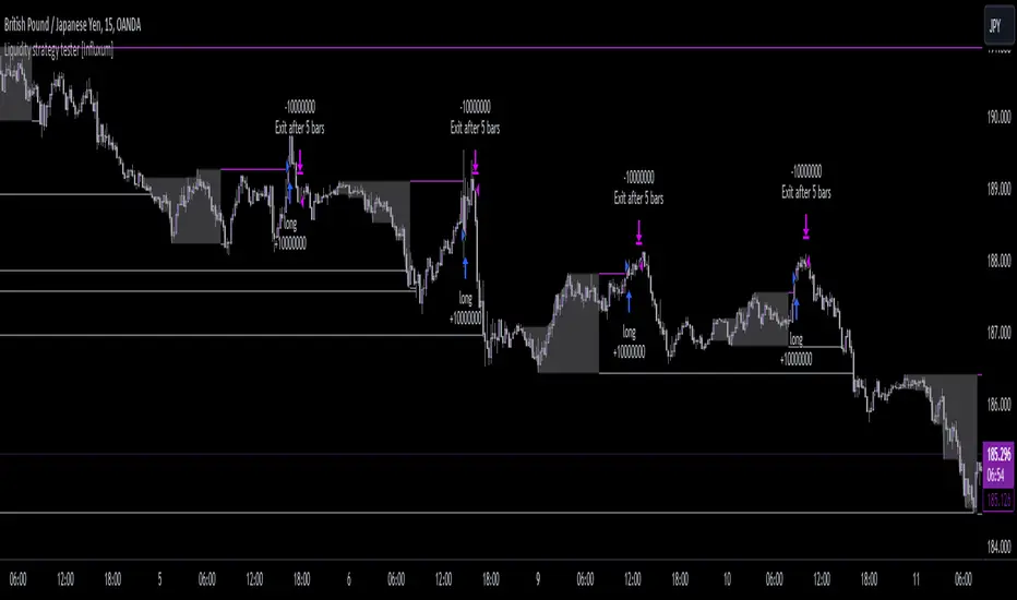
QuantBuilder | FractalystWhat's the strategy's purpose and functionality?
QuantBuilder is designed for both traders and investors who want to utilize mathematical techniques to develop profitable strategies through backtesting on historical data.
The primary goal is to develop profitable quantitive strategies that not only outperform the underlying asset in terms of returns but also minimize drawdown.
For instance, consider Bitcoin (BTC), which has experienced significant volatility, averaging an estimated 200% annual return over the past decade, with maximum drawdowns exceeding -80%. By employing this strategy with diverse entry and exit techniques, users can potentially seek to enhance their Compound Annual Growth Rate (CAGR) while managing risk to maintain a lower maximum drawdown.
While this strategy employs quantitative techniques, including mathematical methods such as probabilities and positive expected values, it demonstrates exceptional efficacy across all markets. It particularly excels in futures, indices, stocks, cryptocurrencies, and commodities, leveraging their inherent trending behaviors for optimized performance.
In both trending and consolidating market conditions, QuantBuilder employs a combination of multi-timeframe probabilities, expected values, directional biases, moving averages and diverse entry models to identify and capitalize on bullish market movements.
How does the strategy perform for both investors and traders?
The strategy has two main modes, tailored for different market participants: Traders and Investors.
1. Trading:
- Designed for traders looking to capitalize on bullish markets.
- Utilizes a percentage risk per trade to manage risk and optimize returns.
- Suitable for both swing and intraday trading with a focus on probabilities and risk per trade approach.
2. Investing:
- Geared towards investors who aim to capitalize on bullish trending markets without using leverage while mitigating the asset's maximum drawdown.
- Utilizes pre-define percentage of the equity to buy, hold, and manage the asset.
- Focuses on long-term growth and capital appreciation by fully/partially investing in the asset during bullish conditions.
How does the strategy identify market structure? What are the underlying calculations?
The strategy utilizes an efficient logic with for loops to pinpoint the first swing candle featuring a pivot of 2, establishing the point at which the break of structure begins.
What entry criteria are used in this script? What are the underlying calculations?
The script utilizes two entry models: BreakOut and fractal.
Underlying Calculations:
Breakout: The script assigns the most recent swing high to a variable. When the price closes above this level and all other conditions are met, the script executes a breakout entry (conservative approach).
Fractal: The script identifies a swing low with a period of 2. Once this condition is met, the script executes the trade (aggressive approach).
How does the script calculate probabilities? What are the underlying calculations?
The script calculates probabilities by monitoring price interactions with liquidity levels. Here’s how the underlying calculations work:
Tracking Price Hits: The script counts the number of times the price taps into each liquidity side after the EQM level is activated. This data is stored in an array for further analysis.
Sample Size Consideration: The total number of price interactions serves as the sample size for calculating probabilities.
Probability Calculation: For each liquidity side, the script calculates the probability by taking the average of the recorded hits. This allows for a dynamic assessment of the likelihood that a particular side will be hit next, based on historical performance.
Dynamic Adjustment: As new price data comes in, the probabilities are recalculated, providing real-time aduptive insights into market behavior.
Note: The calculations are performed independently for each directional range. A range is considered bearish if the previous breakout was through a sellside liquidity. Conversely, a range is considered bullish if the most recent breakout was through a buyside liquidity.
How does the script calculate expected values? What are the underlying calculations?
The script calculates expected values by leveraging the probabilities of winning and losing trades, along with their respective returns. The process involves the following steps:
This quantitative methodology provides a robust framework for assessing the expected performance of trading strategies based on historical data and backtesting results.
How is the contextual bias calculated? What are the underlying calculations?
The contextual bias in the QuantBuilder script is calculated through a structured approach that assesses market structure based on swing highs and lows. Here’s how it works:
Identification of Swing Points: The script identifies significant swing points using a defined pivot logic, focusing on the first swing high and swing low. This helps establish critical levels for determining market structure.
Break of Structure (BOS) Assessment:
Bullish BOS: The script recognizes a bullish break of structure when a candle closes above the first swing high, followed by at least one swing low.
Bearish BOS: Conversely, a bearish break of structure is identified when a candle closes below the first swing low, followed by at least one swing high.
Bias Assignment: Based on the identified break of structure, the script assigns directional biases:
A bullish bias is assigned if a bullish BOS is confirmed.
A bearish bias is assigned if a bearish BOS is confirmed.
Quantitative Evaluation: Each identified bias is quantitatively evaluated, allowing the script to assign numerical values representing the strength of each bias. This quantification aids in assessing the reliability of market sentiment across multiple timeframes.
What's the purpose of using moving averages in this strategy? What are the underlying calculations?
Using moving averages is a widely-used technique to trade with the trend.
The main purpose of using moving averages in this strategy is to filter out bearish price action and to only take trades when the price is trading ABOVE specified moving averages.
The script uses different types of moving averages with user-adjustable timeframes and periods/lengths, allowing traders to try out different variations to maximize strategy performance and minimize drawdowns.
By applying these calculations, the strategy effectively identifies bullish trends and avoids market conditions that are not conducive to profitable trades.
The MA filter allows traders to choose whether they want a specific moving average above or below another one as their entry condition.
What type of stop-loss identification method are used in this strategy? What are the underlying calculations?
- Initial Stop-loss:
1. ATR Based:
The Average True Range (ATR) is a method used in technical analysis to measure volatility. It is not used to indicate the direction of price but to measure volatility, especially volatility caused by price gaps or limit moves.
Calculation:
- To calculate the ATR, the True Range (TR) first needs to be identified. The TR takes into account the most current period high/low range as well as the previous period close.
The True Range is the largest of the following:
- Current Period High minus Current Period Low
- Absolute Value of Current Period High minus Previous Period Close
- Absolute Value of Current Period Low minus Previous Period Close
- The ATR is then calculated as the moving average of the TR over a specified period. (The default period is 14)
2. ADR Based:
The Average Day Range (ADR) is an indicator that measures the volatility of an asset by showing the average movement of the price between the high and the low over the last several days.
Calculation:
- To calculate the ADR for a particular day:
- Calculate the average of the high prices over a specified number of days.
- Calculate the average of the low prices over the same number of days.
- Find the difference between these average values.
- The default period for calculating the ADR is 14 days. A shorter period may introduce more noise, while a longer period may be slower to react to new market movements.
3. PL Based:
This method places the stop-loss at the low of the previous candle.
If the current entry is based on the hunt entry strategy, the stop-loss will be placed at the low of the candle that wicks through the lower FRMA band.
Example:
If the previous candle's low is 100, then the stop-loss will be set at 100.
This method ensures the stop-loss is placed just below the most recent significant low, providing a logical and immediate level for risk management.
- Trailing Stop-Loss:
One of the key elements of this strategy is its ability to detect structural liquidity and structural invalidation levels across multiple timeframes to trail the stop-loss once the trade is in running profits.
By utilizing this approach, the strategy allows enough room for price to run.
By using these methods, the strategy dynamically adjusts the initial stop-loss based on market volatility, helping to protect against adverse price movements while allowing for enough room for trades to develop.
Each market behaves differently across various timeframes, and it is essential to test different parameters and optimizations to find out which trailing stop-loss method gives you the desired results and performance.
What type of break-even and take profit identification methods are used in this strategy? What are the underlying calculations?
For Break-Even:
Percentage (%) Based:
Moves the initial stop-loss to the entry price when the price reaches a certain percentage above the entry.
Calculation:
Break-even level = Entry Price * (1 + Percentage / 100)
Example:
If the entry price is $100 and the break-even percentage is 5%, the break-even level is $100 * 1.05 = $105.
Risk-to-Reward (RR) Based:
Moves the initial stop-loss to the entry price when the price reaches a certain RR ratio.
Calculation:
Break-even level = Entry Price + (Initial Risk * RR Ratio)
For TP1 (Take Profit 1):
- You can choose to set a take profit level at which your position gets fully closed or 50% if the TP2 boolean is enabled.
- Similar to break-even, you can select either a percentage (%) or risk-to-reward (RR) based take profit level, allowing you to set your TP1 level as a percentage amount above the entry price or based on RR.
For TP2 (Take Profit 2):
- You can choose to set a take profit level at which your position gets fully closed.
- As with break-even and TP1, you can select either a percentage (%) or risk-to-reward (RR) based take profit level, allowing you to set your TP2 level as a percentage amount above the entry price or based on RR.
What's the day filter Filter, what does it do?
The day filter allows users to customize the session time and choose the specific days they want to include in the strategy session. This helps traders tailor their strategies to particular trading sessions or days of the week when they believe the market conditions are more favorable for their trading style.
Customize Session Time:
Users can define the start and end times for the trading session.
This allows the strategy to only consider trades within the specified time window, focusing on periods of higher market activity or preferred trading hours.
Select Days:
Users can select which days of the week to include in the strategy.
This feature is useful for excluding days with historically lower volatility or unfavorable trading conditions (e.g., Mondays or Fridays).
Benefits:
Focus on Optimal Trading Periods:
By customizing session times and days, traders can focus on periods when the market is more likely to present profitable opportunities.
Avoid Unfavorable Conditions:
Excluding specific days or times can help avoid trading during periods of low liquidity or high unpredictability, such as major news events or holidays.
What tables are available in this script?
- Summary: Provides a general overview, displaying key performance parameters such as Net Profit, Profit Factor, Max Drawdown, Average Trade, Closed Trades and more.
Total Commission: Displays the cumulative commissions incurred from all trades executed within the selected backtesting window. This value is derived by summing the commission fees for each trade on your chart.
Average Commission: Represents the average commission per trade, calculated by dividing the Total Commission by the total number of closed trades. This metric is crucial for assessing the impact of trading costs on overall profitability.
Avg Trade: The sum of money gained or lost by the average trade generated by a strategy. Calculated by dividing the Net Profit by the overall number of closed trades. An important value since it must be large enough to cover the commission and slippage costs of trading the strategy and still bring a profit.
MaxDD: Displays the largest drawdown of losses, i.e., the maximum possible loss that the strategy could have incurred among all of the trades it has made. This value is calculated separately for every bar that the strategy spends with an open position.
Profit Factor: The amount of money a trading strategy made for every unit of money it lost (in the selected currency). This value is calculated by dividing gross profits by gross losses.
Avg RR: This is calculated by dividing the average winning trade by the average losing trade. This field is not a very meaningful value by itself because it does not take into account the ratio of the number of winning vs losing trades, and strategies can have different approaches to profitability. A strategy may trade at every possibility in order to capture many small profits, yet have an average losing trade greater than the average winning trade. The higher this value is, the better, but it should be considered together with the percentage of winning trades and the net profit.
Winrate: The percentage of winning trades generated by a strategy. Calculated by dividing the number of winning trades by the total number of closed trades generated by a strategy. Percent profitable is not a very reliable measure by itself. A strategy could have many small winning trades, making the percent profitable high with a small average winning trade, or a few big winning trades accounting for a low percent profitable and a big average winning trade. Most mean-reversion successful strategies have a percent profitability of 40-80% but are profitable due to risk management control.
BE Trades: Number of break-even trades, excluding commission/slippage.
Losing Trades: The total number of losing trades generated by the strategy.
Winning Trades: The total number of winning trades generated by the strategy.
Total Trades: Total number of taken traders visible your charts.
Net Profit: The overall profit or loss (in the selected currency) achieved by the trading strategy in the test period. The value is the sum of all values from the Profit column (on the List of Trades tab), taking into account the sign.
- Monthly: Displays performance data on a month-by-month basis, allowing users to analyze performance trends over each month and year.
- Weekly: Displays performance data on a week-by-week basis, helping users to understand weekly performance variations.
- UI Table: A user-friendly table that allows users to view and save the selected strategy parameters from user inputs. This table enables easy access to key settings and configurations, providing a straightforward solution for saving strategy parameters by simply taking a screenshot with Alt + S or ⌥ + S.
User-input styles and customizations:
To facilitate studying historical data, all conditions and filters can be applied to your charts. By plotting background colors on your charts, you'll be able to identify what worked and what didn't in certain market conditions.
Please note that all background colors in the style are disabled by default to enhance visualization.
How to Use This Quantitive Strategy Builder to Create a Profitable Edge and System?
Choose Your Strategy mode:
- Decide whether you are creating an investing strategy or a trading strategy.
Select a Market:
- Choose a one-sided market such as stocks, indices, or cryptocurrencies.
Historical Data:
- Ensure the historical data covers at least 10 years of price action for robust backtesting.
Timeframe Selection:
- Choose the timeframe you are comfortable trading with. It is strongly recommended to use a timeframe above 15 minutes to minimize the impact of commissions/slippage on your profits.
Set Commission and Slippage:
- Properly set the commission and slippage in the strategy properties according to your broker/prop firm specifications.
Parameter Optimization:
- Use trial and error to test different parameters until you find the performance results you are looking for in the summary table or, preferably, through deep backtesting using the strategy tester.
Trade Count:
- Ensure the number of trades is 200 or more; the higher, the better for statistical significance.
Positive Average Trade:
- Make sure the average trade is above zero.
(An important value since it must be large enough to cover the commission and slippage costs of trading the strategy and still bring a profit.)
Performance Metrics:
- Look for a high profit factor, and net profit with minimum drawdown.
- Ideally, aim for a drawdown under 20-30%, depending on your risk tolerance.
Refinement and Optimization:
- Try out different markets and timeframes.
- Continue working on refining your edge using the available filters and components to further optimize your strategy.
What makes this strategy original?
QuantBuilder stands out due to its unique combination of quantitative techniques and innovative algorithms that leverage historical data for real-time trading decisions. Unlike most algorithmic strategies that work based on predefined rules, this strategy adapts to real-time market probabilities and expected values, enhancing its reliability. Key features include:
Mathematical Framework: The strategy integrates advanced mathematical concepts, such as probabilities and expected values, to assess trade viability and optimize decision-making.
Multi-Timeframe Analysis: By utilizing multi-timeframe probabilities, QuantBuilder provides a comprehensive view of market conditions, enhancing the accuracy of entry and exit points.
Dynamic Market Structure Identification: The script employs a systematic approach to identify market structure changes, utilizing a blend of swing highs and lows to detect contextual/direction bias of the market.
Built-in Trailing Stop Loss: The strategy features a dynamic trailing stop loss based on multi-timeframe analysis of market structure. This allows traders to lock in profits while adapting to changing market conditions, ensuring that exits are executed at optimal levels without prematurely closing positions.
Robust Performance Metrics: With detailed performance tables and visualizations, users can easily evaluate strategy effectiveness and adjust parameters based on historical performance.
Adaptability: The strategy is designed to work across various markets and timeframes, making it versatile for different trading styles and objectives.
Suitability for Investors and Traders: QuantBuilder is ideal for both investors and traders looking to rely on mathematically proven data to create profitable strategies, ensuring that decisions are grounded in quantitative analysis.
These original elements combine to create a powerful tool that can help both traders and investors to build and refine profitable strategies based on algorithmic quantitative analysis.
Terms and Conditions | Disclaimer
Our charting tools are provided for informational and educational purposes only and should not be construed as financial, investment, or trading advice. They are not intended to forecast market movements or offer specific recommendations. Users should understand that past performance does not guarantee future results and should not base financial decisions solely on historical data.
Built-in components, features, and functionalities of our charting tools are the intellectual property of @Fractalyst Unauthorized use, reproduction, or distribution of these proprietary elements is prohibited.
By continuing to use our charting tools, the user acknowledges and accepts the Terms and Conditions outlined in this legal disclaimer and agrees to respect our intellectual property rights and comply with all applicable laws and regulations.

Grok/Claude Turtle Soup Strategy # 🥣 Turtle Soup Strategy (Enhanced)
## A Mean-Reversion Strategy Based on Failed Breakouts
---
## Historical Origins
### The Original Turtle Traders (1983-1988)
The Turtle Trading system is one of the most famous experiments in trading history. In 1983, legendary commodities trader **Richard Dennis** made a bet with his partner **William Eckhardt** about whether great traders were born or made. Dennis believed trading could be taught; Eckhardt believed it was innate.
To settle the debate, Dennis recruited 23 ordinary people through newspaper ads—including a professional blackjack player, a fantasy game designer, and an accountant—and taught them his trading system in just two weeks. He called them "Turtles" after turtle farms he had visited in Singapore, saying *"We are going to grow traders just like they grow turtles in Singapore."*
The results were extraordinary. Over the next five years, the Turtles reportedly earned over **$175 million in profits**. The experiment proved Dennis right: trading could indeed be taught.
#### The Original Turtle Rules:
- **Entry:** Buy when price breaks above the 20-day high (System 1) or 55-day high (System 2)
- **Exit:** Sell when price breaks below the 10-day low (System 1) or 20-day low (System 2)
- **Stop Loss:** 2x ATR (Average True Range) from entry
- **Position Sizing:** Based on volatility (ATR)
- **Philosophy:** Pure trend-following—catch big moves by riding breakouts
The Turtle system was a **trend-following** strategy that assumed breakouts would lead to sustained trends. It worked brilliantly in trending markets but suffered during choppy, range-bound conditions.
---
### The Turtle Soup Strategy (1990s)
In the 1990s, renowned trader **Linda Bradford Raschke** (along with Larry Connors) observed something interesting: many of the breakouts that the Turtle system traded actually *failed*. Price would spike above the 20-day high, trigger Turtle buy orders, then immediately reverse—trapping the breakout traders.
Raschke realized these failed breakouts were predictable and tradeable. She developed the **Turtle Soup** strategy, which does the *exact opposite* of the original Turtle system:
> *"Instead of buying the breakout, we wait for it to fail—then fade it."*
The name "Turtle Soup" is a clever play on words: the strategy essentially "eats" the Turtles by trading against them when their breakouts fail.
#### Original Turtle Soup Rules:
- **Setup:** Price makes a new 20-day high (or low)
- **Qualifier:** The previous 20-day high must be at least 3-4 days old (not a fresh breakout)
- **Entry Trigger:** Price reverses back inside the channel (failed breakout)
- **Entry:** Go SHORT (against the failed breakout above), or LONG (against the failed breakdown below)
- **Philosophy:** Mean-reversion—fade false breakouts and profit from trapped traders
#### Turtle Soup Plus One Variant:
Raschke also developed a more conservative variant called "Turtle Soup Plus One" which waits for the *next bar* after the breakout to confirm the failure before entering. This reduces false signals but may miss some opportunities.
---
## Our Enhanced Turtle Soup Strategy
We have taken the classic Turtle Soup concept and enhanced it with modern technical indicators and filters to improve signal quality and adapt to today's markets.
### Core Logic Preserved
The fundamental strategy remains true to Raschke's original concept:
| Turtle (Original) | Turtle Soup (Our Strategy) |
|-------------------|---------------------------|
| BUY breakout above 20-day high | SHORT when that breakout FAILS |
| SELL breakout below 20-day low | LONG when that breakdown FAILS |
| Trend-following | Mean-reversion |
| "The trend is your friend" | "Failed breakouts trap traders" |
---
### Enhancements & Improvements
#### 1. RSI Exhaustion Filter
**Addition:** RSI must confirm exhaustion before entry
- **For SHORT entries:** RSI > 60 (buyers exhausted)
- **For LONG entries:** RSI < 40 (sellers exhausted)
**Why:** The original Turtle Soup had no momentum filter. Adding RSI ensures we only fade breakouts when the market is showing signs of exhaustion, significantly reducing false signals. This enhancement was inspired by later traders who found RSI extremes (originally 90/10, softened to 60/40) dramatically improved win rates.
#### 2. ADX Trending Filter
**Addition:** ADX must be > 20 for trades to execute
**Why:** While the original Turtle Soup was designed for ranging markets, we found that requiring *some* trend strength (ADX > 20) actually improves results. This ensures we're trading in markets with enough directional movement to create meaningful failed breakouts, rather than random noise in dead markets.
#### 3. Heikin Ashi Smoothing
**Addition:** Optional Heikin Ashi calculations for breakout detection
**Why:** Heikin Ashi candles smooth out price noise and make trend reversals more visible. When enabled, the strategy uses HA values to detect breakouts and failures, reducing whipsaws from erratic price spikes.
#### 4. Dynamic Donchian Channels with Regime Detection
**Addition:** Color-coded channels based on market regime
- 🟢 **Green:** Bullish regime (uptrend + DI+ > DI- + OBV bullish)
- 🔴 **Red:** Bearish regime (downtrend + DI- > DI+ + OBV bearish)
- 🟡 **Yellow:** Neutral regime
**Why:** Visual regime detection helps traders understand the broader market context. The original Turtle Soup had no regime awareness—our enhancement lets traders see at a glance whether conditions favor the strategy.
#### 5. Volume Spike Detection (Optional)
**Addition:** Optional filter requiring volume surge on the breakout bar
**Why:** Failed breakouts are more significant when they occur on high volume. A volume spike on the breakout bar (default 1.2x average) indicates more traders got trapped, creating stronger reversal potential.
#### 6. ATR-Based Stops and Targets
**Addition:** Configurable ATR-based stop losses and profit targets
- **Stop Loss:** 1.5x ATR (default)
- **Profit Target:** 2.0x ATR (default)
**Why:** The original Turtle Soup used fixed stop placement. ATR-based stops adapt to current volatility, providing tighter stops in calm markets and wider stops in volatile conditions.
#### 7. Signal Cooldown
**Addition:** Minimum bars between trades (default 5)
**Why:** Prevents overtrading during choppy conditions where multiple failed breakouts might occur in quick succession.
#### 8. Real-Time Info Panel
**Addition:** Comprehensive dashboard showing:
- Current regime (Bullish/Bearish/Neutral)
- RSI value and zone
- ADX value and trending status
- Breakout status
- Bars since last high/low
- Current setup status
- Position status
**Why:** Gives traders instant visibility into all strategy conditions without needing to check multiple indicators.
---
## Entry Rules Summary
### SHORT Entry (Fading Failed Breakout Above)
1. ✅ Price breaks ABOVE the 20-period Donchian high
2. ✅ Previous 20-period high was at least 1 bar ago
3. ✅ Price closes back BELOW the Donchian high (failed breakout)
4. ✅ RSI > 60 (exhausted buyers)
5. ✅ ADX > 20 (trending market)
6. ✅ Cooldown period met
→ **Enter SHORT**, betting the breakout will fail
### LONG Entry (Fading Failed Breakdown Below)
1. ✅ Price breaks BELOW the 20-period Donchian low
2. ✅ Previous 20-period low was at least 1 bar ago
3. ✅ Price closes back ABOVE the Donchian low (failed breakdown)
4. ✅ RSI < 40 (exhausted sellers)
5. ✅ ADX > 20 (trending market)
6. ✅ Cooldown period met
→ **Enter LONG**, betting the breakdown will fail
---
## Exit Rules
1. **ATR Stop Loss:** Position closed if price moves 1.5x ATR against entry
2. **ATR Profit Target:** Position closed if price moves 2.0x ATR in favor
3. **Channel Exit:** Position closed if price breaks the exit channel in the opposite direction
4. **Mid-Channel Exit:** Position closed if price returns to channel midpoint
---
## Best Market Conditions
The Turtle Soup strategy performs best when:
- ✅ Markets are prone to false breakouts
- ✅ Volatility is moderate (not too low, not extreme)
- ✅ Price is oscillating within a broader range
- ✅ There are clear support/resistance levels
The strategy may struggle when:
- ❌ Strong trends persist (breakouts follow through)
- ❌ Volatility is extremely low (no meaningful breakouts)
- ❌ Markets are in news-driven directional moves
---
## Default Settings
| Parameter | Default | Description |
|-----------|---------|-------------|
| Lookback Period | 20 | Donchian channel period |
| Min Bars Since Extreme | 1 | Bars since last high/low |
| RSI Length | 14 | RSI calculation period |
| RSI Short Level | 60 | RSI must be above this for shorts |
| RSI Long Level | 40 | RSI must be below this for longs |
| ADX Length | 14 | ADX calculation period |
| ADX Threshold | 20 | Minimum ADX for trades |
| ATR Period | 20 | ATR calculation period |
| ATR Stop Multiplier | 1.5 | Stop loss distance in ATR |
| ATR Target Multiplier | 2.0 | Profit target distance in ATR |
| Cooldown Period | 5 | Minimum bars between trades |
| Volume Multiplier | 1.2 | Volume spike threshold |
---
## Philosophy
> *"The Turtle system made millions by following breakouts. The Turtle Soup strategy makes money when those breakouts fail. In trading, there's always someone on the other side of the trade—this strategy profits by being the smart money that fades the trapped breakout traders."*
The beauty of the Turtle Soup strategy is its elegant simplicity: it exploits a known, repeatable pattern (failed breakouts) while using modern filters (RSI, ADX) to improve timing and reduce false signals.
---
## Credits
- **Original Turtle System:** Richard Dennis & William Eckhardt (1983)
- **Turtle Soup Strategy:** Linda Bradford Raschke & Larry Connors (1990s)
- **RSI Enhancement:** Various traders who discovered RSI extremes improve reversal detection
- **This Implementation:** Enhanced with Heikin Ashi smoothing, regime detection, ADX filtering, and comprehensive visualization
---
*"We're not following the turtles—we're making soup out of them."* 🥣

Liquidity SweeperStrategy Overview
This Pine Script implements a Liquidity Sweep Trading Strategy, a sophisticated approach that capitalizes on market manipulation tactics commonly used by institutional traders. The strategy identifies when price "sweeps" above recent swing highs or below swing lows to trigger stop losses and grab liquidity, then quickly reverses direction - creating high-probability trading opportunities.
Core Concept: What is a Liquidity Sweep?
A liquidity sweep occurs when:
Price breaks above a swing high (or below a swing low) to trigger retail stop losses
Institutional players absorb this liquidity at favorable prices
Price quickly reverses back into the previous range
This creates a "fake breakout" or "stop hunt" pattern
The strategy exploits these manipulative moves by entering trades in the direction of the reversal.
How the Strategy Works
1. Swing Point Detection
Uses a lookback period (default: 20 bars) to identify significant swing highs and lows
Employs proper pivot point detection using ta.highestbars() and ta.lowestbars()
Only considers confirmed swing points (not just recent highs/lows)
2. Liquidity Sweep Identification
High Sweep (Short Setup):
Price moves above the last swing high (triggering buy stops)
Same bar closes back below the swing high (showing rejection)
Low Sweep (Long Setup):
Price moves below the last swing low (triggering sell stops)
Same bar closes back above the swing low (showing support)
3. Confirmation Process
Requires price to stay within the swept range for a specified number of bars (default: 3)
This confirms the sweep was genuine and not just normal volatility
Prevents false signals and improves trade quality
4. Entry Logic
Long Entries: Triggered after confirmed low sweeps
Short Entries: Triggered after confirmed high sweeps
5. Risk Management
Stop Loss: Placed at a multiple of ATR (default: 1.5x) from entry price
Take Profit: Risk/Reward ratio based (default: 2:1)
Position Sizing: 10% of equity per trade (configurable)
Red X-crosses: High sweeps detected
Green X-crosses: Low sweeps detected
Red triangles (down): Short entry signals
Green triangles (up): Long entry signals
Horizontal lines: Current swing high/low levels
Info label: Shows last detected swing levels
Optimal Conditions:
Timeframes: 1H, 4H, and Daily work best
Market Conditions: Ranging and trending markets both suitable
Volatility: Moderate to high volatility preferred
Session Times: Most effective during active trading sessions
Strengths:
✅ Exploits institutional manipulation tactics
✅ Clear entry/exit rules with defined risk
✅ Works across multiple asset classes
✅ Includes proper confirmation to reduce false signals
✅ Visual clarity for manual verification
✅ Reasonable risk/reward parameters
Limitations:
⚠️ Requires patience - not a high-frequency strategy
⚠️ Market dependent - fewer signals in low volatility periods
⚠️ Needs sufficient lookback data for swing identification
⚠️ May have drawdown periods during strong trending moves
⚠️ Requires understanding of market structure concepts
Best Practices for Users
Optimization Tips:
Adjust lookback period based on timeframe (shorter for lower TFs)
Test different confirmation periods for your market
Consider market session times when backtesting
Use alongside volume analysis for additional confirmation
Risk Management:
Never risk more than 2-3% per trade of total capital
Consider reducing position size during high-impact news
Monitor correlation if trading multiple pairs simultaneously
Use additional filters (trend, support/resistance) for confluence
Backtesting Recommendations:
Test on at least 6 months of historical data
Include different market conditions (trending, ranging, volatile)
Consider transaction costs and slippage in results
Forward test on demo before live implementation
Expected Results
Based on typical liquidity sweep strategy performance:
Disclaimer
This strategy is based on market structure analysis and institutional trading behavior patterns. Past performance doesn't guarantee future results. Users should:
Thoroughly backtest before live trading
Start with small position sizes
Understand the underlying concepts before implementation
Consider combining with other analysis methods
Always use proper risk management
The strategy works best when traders understand the psychological and structural elements of liquidity sweeps rather than just following signals blindly.
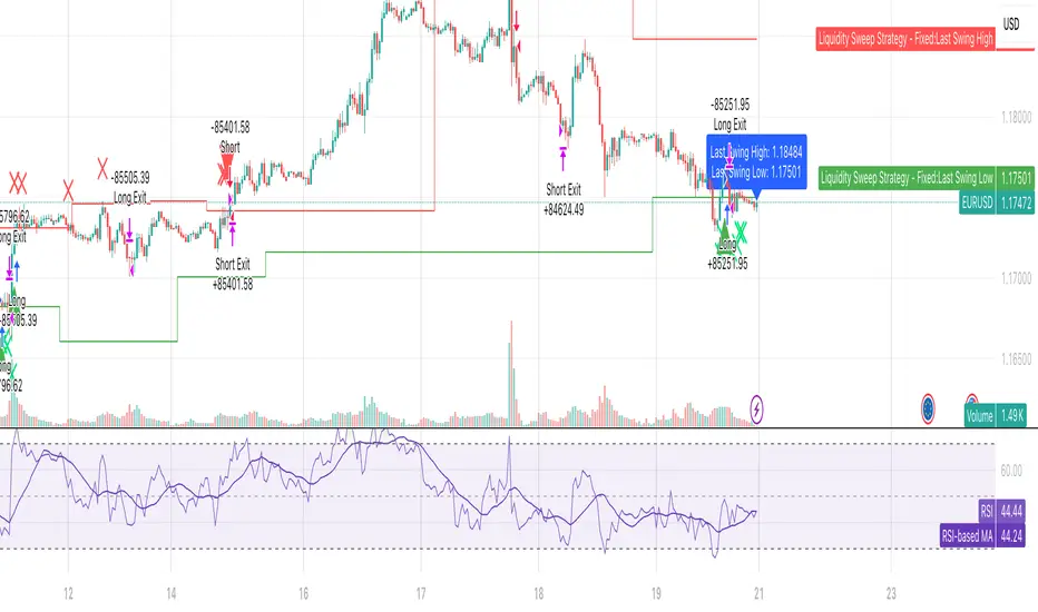
TheHorsyAlgoPROThe Horsy algo is an automated strategy that uses any minute Higher timeframe range as reference and search for a purge of liquidity on the HTF high or low where buyside or sell side liquidity is, the algo only search this at specific desired times that can be configured according to the time you usually trade, the strategy is known as Turtle soup purge and reverse or lately as CRT.
Why is useful?
The purpose of this Algorithm is to help turtle soup traders to quickly identify when the market is likely to reverse the algo evaluates if the opportunity is worth it, base on risk reward and other desired filters. Also this strategy can help to quickly backtest the trader strategy it can be configured in different timeframes and adapt to the trader personality, they can easily see the results and statistics and notice if its profitable or not.
This algo is useful for intraday traders looking for a purge and reverse at a key times and at key HTF price levels this only looks the previous HTF highs and lows but is important to also monitor Order blocks, FVGs, gaps, or wicks to have the best results.
How it works and how it does it?
The Horsy algo simply Jumps from one type of liquidity to another one buyside to sell side or vice versa. In order for the algo to trigger an entry it has to meet these conditions
1. Take HTF liquidity, trade above a HTF high or below a HTF low in the selected time window
2. Make a change in the state of delivery with a close below the previous candle low for shorts and close above previous candle high for longs.
3. Allow for a reasonable risk reward, it will use the highest high for shorts and the lowest low for longs. The default take profit is the opposite side of the range.
4. Validate others user filters this include enter only trades aligned with the HTF bias, or trades aligned with the LTF bias or booth. The algo have the option to enter only premium and discount entries. And finally, an option to allow for different contract sizes depending of the maximum percent of the account we want to risk default is 1%. For this last option is important to check the initial balance and leverage are configured correctly, is disable by default because it requires more capital to perform well.
We can see the algo performing in the picture below with a short trade, notice there are some white lines, they are the high or the low of HTF candle that start generating inside candles in the HTF meaning a possible consolidation. The algo plots the HTF ranges in a shaded boxes as you can see below
The HTF bias as you can see in the picture is calculated based on the last close of the HTF meaning close above previous HTF high is bullish close below previous HTF low is bearish. This HTF bias level is also the last HTF mid-price or 50%. By default, this line is enabled.
The LTF bias is calculated based on the range created from the expansion outside the previous HTF range is also the mid-price. If the LTF close above previous HTF high is bullish and if the LTF close below previous HTF low is bearish. By default this LTF bias line is disable.
This strategy includes an original and personal developed code that uses dealing ranges to recognize if the market is expanding, retracing, reversing or consolidating. This allow the algo to exit the position when it detects a retracement or at the end of the expansion. This is the default exit type.
You can monitor the previous dealing ranges created in history with an option than can be enable, by default is disable, this ranges are created after price takes buyside and then sell side or vice versa. So this dealing ranges can be useful also to identify minor pools of liquidity and premium and discount in the lower timeframe.
The picture below is a long example, the exit in this case is just at the high of the range. The normal take profit is in a blue line for longs.
How to use it?
First select the desired HTF timeframe recommended is from 30min to 240min then you setup the chart on the lower timeframe you want to trade recommended is from 1min to 15min to enter. By default This strategy is designed to work for intraday during key times when price take stops and then moves quickly away from them. You can select as much as 6 different times or just one. After you select the desired time window where the algo will look for the purge and reverse, They are highlighted in the candles that change colors excluding the gray ones that indicates consolidation.
Then the Algo allow to performs several additional filters in the entries you can select if you want to trade only longs or shorts trades, you can select when to move the stop loss to Break even. In deviations of the risk or you can just select to remove risk when price hits the 50% of previous HTF range.
You can select the minimum desired risk reward of the trade before is allow to be taken. Once is configured correctly the algo should trigger signals with a triangle up or down plus the strategy entry.
At the beginning of the picture there are some blue lines in the HTF high low and close, this is to easily identify that the market is in the Asia session, the time can be configured by the user, these lines are normally gray.
On the right top of the screen you can see some statistics about the strategy how many trades it took, ARR is an approximated value of the accumulated total risk reward of all the trades when they get closed in the simulation.
Profit factor and percent profitable are also shown should be green it means that the strategy makes money over time. But apart from that is important to notice how it makes money it is stable over time? it is a roller coaster? that why I Include this other measurements MxcsTps is the maximum consecutives take profits and Mxcsls is the maximum consecutive stop losses it takes, the slash number after it is the consecutive Break evens. So this way you know what to expect and what is normal in the strategy.
The algo shows all the times the stop loss, take profit and break even level if enable in the colored red lines for short and blue lines for longs. You can also select how price will manage the profit or stoploss point meaning that you can choose to wait for the candle to close to invalidate your idea or to take profit. This is good to avoid liquidity sweeps but can also lead to mayor loses if the idea is wrong. The default setting is to close the trade when price takes the high or low where the stoploss is, the take profit is taken after a retracement to allow to profit on expansions. You can select also to exit on a reversal if you want to ride all the move. This last option has to be used with caution because sometimes price just retrace or reverse very fast decreasing the trade profit and overall strategy performance.
The algo have the option to use standard deviation from the normal risk if you prefer to prevent liquidity sweeps near the stop level this make wider stops but can lead to increased loses so it has to be used carefully.
Below is a picture that show the entry stop and take profit levels with an exit on a retracement activated.
Strategy Results
The backtesting results are obtained simulating a 2000usd account in the Micro Nasdaq using 1 contract per trade. Commission are set to 2usd per contract, slippage to 1tick. You can see in list of trades we are not risking more than 1 % percent of the account. The backtested range is from august to November 2024. This strategy doesn’t generate too much trades because of the time filters and conditions that has to be meet to take an entry but you can see the results of the last 4months with the available data that are around 32 trades.
The default settings for this strategy is HTF as 240min designed to work on a LTF 5min chart, the default purge times are 245-300, 745-800, 845-900, 1045-1100 and 1245-1300 UTC-4, the algo will look for shorts or longs, with a minimum risk reward of 2.0. With an additional filter of the HTFBias. The take profit is by default taken on the first retracement after hitting the target. The default settings are optimized to work on the Nasdaq or Spy, but can also perform well in other assets with the correct adjustments.
Remember entries constitute only a small component of a complete winning strategy. Other factors like risk management, position-sizing, trading frequency, trading fees, and many others must also be properly managed to achieve profitability. Past performance doesn’t guarantee future results. To really take advantage of this strategy you have to study turtle soup and the HTF key levels use this only as a confirmation that your overall idea will play out and use it to backtest your model.
Summary of features
·Adaptable strategy to different HTF timeframes from 1-1440min
· Select up to 6 different purge time windows UTC-4, UTC-5
· Choose desired Risk Reward per trade
· Easily see the HTF high low close and 50% key levels in the LTF
· Identify HTF consolidations that generate key major liquidity pools
· HTF/LTF bias filters to trade in favor of the big trend or in sync
· Shaded boxes that indicate if the market is bullish, bearish or consolidating
· See the current midpoint of the last expansion move
· Optimal trade entry filter to trade only in a discount or premium
· Customizable trade management take profit, stop, breakeven level
· Option to exit on a close, retracement or reversal after hitting the take profit level
· Option to exit on a close or reversal after hitting stop loss
· Configurable breakeven point with standard deviations or at 50% of the HTF
· Calculate different contract sizes depending of a percentage of the initial balance
· Standard deviations from normal risk can be used to prevent liquidity sweeps
· See dealing ranges history to check minor pools of liquidity and premium or discount
· Dashboard with instant statistics about the strategy current settings

InvoTrading - Swing High and Low with BreakoutInvoTrading - Swing High and Low with Breakout Strategy
This strategy is designed to identify trading opportunities based on swing highs and lows, combined with breakout confirmations. It utilizes pivot points to detect potential reversal levels and initiates trades when the price breaks out of these levels under specific conditions.
Key Features:
- Pivot Points: The strategy calculates pivot highs and lows using customizable left and right bars. These pivots represent potential swing points in the market.
- Breakout Detection: It monitors for breakouts above pivot highs (Bullish Break of Structure - BOS) and below pivot lows (Bearish Break of Structure).
- Strong Swings (Optional): You can enable "Strong Swing" detection, which considers only those pivots where the price attempted but failed to break the pivot level, indicating stronger support or resistance.
- Trade Management: The strategy sets entry points, stop losses, and take profits based on a customizable risk-reward ratio.
- Trade Table: An optional table displays recent trades, including their status (Pending, Success, or Failed).
- Visual Aids: Customizable colors and line settings help visualize pivot points, strong swings, and breakout candles on the chart.
---
Settings:
1. Pivot Settings:
- Left Bars: Number of bars to the left of the pivot point (default: 5).
- Right Bars: Number of bars to the right of the pivot point (default: 5).
- Pivot Based On: Choose between "High/Low" or "Close" prices for pivot calculations.
2. Color Settings:
- Pivot High Color: Color for Pivot High markers (default: Blue).
- Pivot Low Color: Color for Pivot Low markers (default: Red).
- Strong Swing High Color: Color for Strong Swing High markers (default: Black).
- Strong Swing Low Color: Color for Strong Swing Low markers (default: Black).
- Breakout Candle Color (BOS): Color for the breakout candle (default: Yellow).
3. Line Settings:
- Line Width: Width of the pivot lines (default: 1).
- Line Length (Bars): Length of the pivot lines in bars (default: 20).
- Maximum Number of Lines to Keep: Limits the number of pivot lines displayed to avoid clutter (default: 100).
4. Trade Settings:
- Enable Buy and Sell Signals: Activates trade entries and exits on the chart (default: False).
- Show Trades Table: Displays a table summarizing recent trades (default: False).
- Risk-Reward Ratio: Sets the desired risk-reward ratio for trades (default: 1.5).
- Number of Trades to Display: Maximum number of recent trades shown in the table (default: 5).
- Enable Strong Trade: Only triggers trades when a "Strong Swing" is detected (default: False).
---
How It Works:
- Pivot Detection: The script identifies pivot highs and lows based on the specified number of left and right bars.
- Strong Swings: If enabled, the strategy marks a pivot as a strong swing if the price attempts to break it but closes back within the pivot level.
- Breakout Confirmation:
- Long Entry: Occurs when the price closes above a pivot high, signaling a bullish breakout. If "Strong Trade" is enabled, it must be a strong swing high.
- Short Entry: Occurs when the price closes below a pivot low, signaling a bearish breakout. If "Strong Trade" is enabled, it must be a strong swing low.
- Trade Execution: Upon a valid breakout, the strategy places a trade with a stop loss set at the previous candle's low (for longs) or high (for shorts). The take profit is calculated based on the specified risk-reward ratio.
- Trade Monitoring: The strategy updates the status of each trade (Pending, Success, Failed) based on whether the take profit or stop loss is hit.
- Visualization: Breakout candles are highlighted, and pivot lines are drawn with customizable colors and widths. Strong swings are marked distinctly.
---
Usage Tips:
- Backtesting: Before using this strategy live, backtest it on different time frames and instruments to assess its performance.
- Customization: Adjust the pivot settings and risk-reward ratio to match your trading style and the volatility of the instrument you're trading.
- Risk Management: Always use proper risk management techniques, even though the strategy calculates stop losses and take profits.
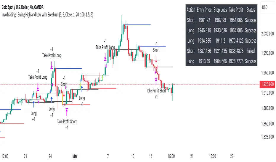
Liquidity Sweep & FVG StrategyThis strategy combines higher-timeframe liquidity levels, stop-hunt (sweep) logic, Fair Value Gaps (FVGs) and structure-based take-profits into a single execution engine.
It is not a simple mash-up of indicators: every module (HTF levels, sweeps, FVGs, ZigZag, sessions) feeds the same entry/exit logic.
1. Core Idea
The script looks for situations where price:
Sweeps a higher-timeframe high/low (takes liquidity around obvious levels),
Then forms a displacement candle with a gap (FVG) in the opposite direction,
Then uses the edge of that FVG as a limit entry,
And manages exits using unswept structural levels (ZigZag swings or HTF levels) as targets.
The intent is to systematically trade failed breakouts / stop hunts with a defined structure and risk model.
It is a backtesting / study tool, not a signal service.
2. How the Logic Works (Conceptual)
a) Higher-Timeframe Liquidity Engine
Daily, Weekly and Monthly highs/lows are pulled via request.security() and stored as HTF liquidity levels.
Each level is drawn as a line with optional label (1D/1W/1M High/Low).
A level is marked as “swept” once price trades through it; swept levels may be removed or shortened depending on settings.
b) Sweep & Manipulation Filter
A low sweep occurs when the current low trades through a stored HTF low.
A high sweep occurs when the current high trades through a stored HTF high.
If both a high and a low are swept in the same bar, the script flags this as “manipulation” and blocks new entries around that noise.
The script also tracks the sweep wick, bar index and HTF timeframe for later use in SL placement and labels.
c) FVG Detection & Management
FVGs are defined using a 3-candle displacement model:
Bullish FVG: high < low
Bearish FVG: low > high
Only gaps larger than a minimum size (ATR-based if no manual value is set) are kept.
FVGs are stored in arrays as boxes with: top, bottom, mid (CE), direction, and state (filled / reclaimed).
Boxes are auto-extended and visually faded when price is far away, or deleted when filled.
d) Entry Conditions (Sweep + FVG)
For each recent sweep window:
After a low sweep, the script searches for the nearest bullish FVG below price and uses its top edge as a long limit entry.
After a high sweep, it searches for the nearest bearish FVG above price and uses its bottom edge as a short limit entry.
A “knife protection” check blocks trades where price is already trading through the proposed stop.
Only one entry per sweep is allowed; entries are only placed inside the configured NY trading sessions and only if no manipulation flag is active and EOD protection allows it.
e) Stop-Loss Placement (“Tick-Free” SL)
The stop is not placed directly on the HTF level; instead, the script scans a window around the sweep bar to find a local extreme:
Longs: lowest low in a configurable bar window around the sweep.
Shorts: highest high in that window.
This produces a structure-based SL that is generally outside the main sweep wick.
f) Take-Profit Logic (ZigZag + HTF Levels)
A lightweight ZigZag engine tracks swing highs/lows and removes levels that have already been broken.
For intraday timeframes (< 1h), TP candidates come from unswept ZigZag swings above/below the entry.
For higher timeframes (≥ 1h), TP candidates fall back to unswept HTF liquidity levels.
The script picks up to two targets:
TP1: nearest valid target in the trade direction (or a 2R fallback if none exists),
TP2: second target (or a 4R fallback if none exists).
A multi-TP model is used: typically 50% at TP1, remainder managed towards TP2 with breakeven plus offset once TP1 is hit.
g) Session & End-of-Day Filters
Three predefined NY sessions (Early, Open, Afternoon) are available; entries are only allowed inside active sessions.
An End-of-Day filter checks a user-defined NY close time and:
Blocks new entries close to the end of the day,
Optionally forces flat before the close.
3. Inputs Overview (Conceptual)
Liquidity settings: which HTF levels to track (1D/1W/1M), how many to show, and sweep priority (highest TF vs nearest vs any).
FVG settings: visibility radius, search window after a sweep, minimum FVG size.
ZigZag settings: swing length used for TP discovery.
Execution & protection: limit order timeout, breakeven offset, EOD protection.
Visuals: labels, sweep markers, manipulation warning, session highlighting, TP lines, etc.
For exact meaning of each input, please refer to the inline comments in the open-source code.
4. Strategy Properties & Backtesting Notes
Default strategy properties in this script:
Initial capital: 100,000
Order size: 10% of equity (strategy.percent_of_equity)
Commission: 0.01% per trade (adjust as needed for your broker/asset)
Slippage: must be set manually in the Strategy Tester (recommended: at least a few ticks on fast markets).
Even though the order size is 10% of equity, actual risk per trade depends on the SL distance and is typically much lower than 10% of the account. You should still adjust these values to keep risk within what you personally consider sustainable (e.g. somewhere in the 1–2% range per trade).
For more meaningful results:
Test on liquid instruments (e.g. major indices, FX, or liquid futures).
Use enough history to reach 100+ closed trades on your market/timeframe.
Always include realistic commission and slippage.
Do not assume that past performance will continue.
5. How to Use
Apply the strategy to your preferred symbol and timeframe.
Set broker-like commission and slippage in the Strategy Tester.
Adjust:
HTF levels (1D/1W/1M),
Sessions (NY windows),
FVG search window and minimum size,
ZigZag length and EOD filter.
Observe how entries only appear:
After a HTF sweep,
In the configured session,
At a FVG edge,
With TP lines anchored at unswept structure / liquidity.
Use this primarily as a research and backtesting tool to study how your own ICT / SMC ideas behave over a large sample of trades.
6. Disclaimer
This script is for educational and research purposes only.
It does not constitute financial advice, and it does not guarantee profitability. Always validate results with realistic assumptions and use your own judgment before trading live.
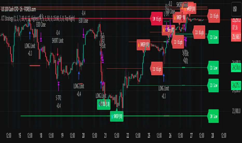
Bober XM v2.0# ₿ober XM v2.0 Trading Bot Documentation
**Developer's Note**: While our previous Bot 1.3.1 was removed due to guideline violations, this setback only fueled our determination to create something even better. Rising from this challenge, Bober XM 2.0 emerges not just as an update, but as a complete reimagining with multi-timeframe analysis, enhanced filters, and superior adaptability. This adversity pushed us to innovate further and deliver a strategy that's smarter, more agile, and more powerful than ever before. Challenges create opportunity - welcome to Cryptobeat's finest work yet.
## !!!!You need to tune it for your own pair and timeframe and retune it periodicaly!!!!!
## Overview
The ₿ober XM v2.0 is an advanced dual-channel trading bot with multi-timeframe analysis capabilities. It integrates multiple technical indicators, customizable risk management, and advanced order execution via webhook for automated trading. The bot's distinctive feature is its separate channel systems for long and short positions, allowing for asymmetric trade strategies that adapt to different market conditions across multiple timeframes.
### Key Features
- **Multi-Timeframe Analysis**: Analyze price data across multiple timeframes simultaneously
- **Dual Channel System**: Separate parameter sets for long and short positions
- **Advanced Entry Filters**: RSI, Volatility, Volume, Bollinger Bands, and KEMAD filters
- **Machine Learning Moving Average**: Adaptive prediction-based channels
- **Multiple Entry Strategies**: Breakout, Pullback, and Mean Reversion modes
- **Risk Management**: Customizable stop-loss, take-profit, and trailing stop settings
- **Webhook Integration**: Compatible with external trading bots and platforms
### Strategy Components
| Component | Description |
|---------|-------------|
| **Dual Channel Trading** | Uses either Keltner Channels or Machine Learning Moving Average (MLMA) with separate settings for long and short positions |
| **MLMA Implementation** | Machine learning algorithm that predicts future price movements and creates adaptive bands |
| **Pivot Point SuperTrend** | Trend identification and confirmation system based on pivot points |
| **Three Entry Strategies** | Choose between Breakout, Pullback, or Mean Reversion approaches |
| **Advanced Filter System** | Multiple customizable filters with multi-timeframe support to avoid false signals |
| **Custom Exit Logic** | Exits based on OBV crossover of its moving average combined with pivot trend changes |
### Note for Novice Users
This is a fully featured real trading bot and can be tweaked for any ticker — SOL is just an example. It follows this structure:
1. **Indicator** – gives the initial signal
2. **Entry strategy** – decides when to open a trade
3. **Exit strategy** – defines when to close it
4. **Trend confirmation** – ensures the trade follows the market direction
5. **Filters** – cuts out noise and avoids weak setups
6. **Risk management** – controls losses and protects your capital
To tune it for a different pair, you'll need to start from scratch:
1. Select the timeframe (candle size)
2. Turn off all filters and trend entry/exit confirmations
3. Choose a channel type, channel source and entry strategy
4. Adjust risk parameters
5. Tune long and short settings for the channel
6. Fine-tune the Pivot Point Supertrend and Main Exit condition OBV
This will generate a lot of signals and activity on the chart. Your next task is to find the right combination of filters and settings to reduce noise and tune it for profitability.
### Default Strategy values
Default values are tuned for: Symbol BITGET:SOLUSDT.P 5min candle
Filters are off by default: Try to play with it to understand how it works
## Configuration Guide
### General Settings
| Setting | Description | Default Value |
|---------|-------------|---------------|
| **Long Positions** | Enable or disable long trades | Enabled |
| **Short Positions** | Enable or disable short trades | Enabled |
| **Risk/Reward Area** | Visual display of stop-loss and take-profit zones | Enabled |
| **Long Entry Source** | Price data used for long entry signals | hl2 (High+Low/2) |
| **Short Entry Source** | Price data used for short entry signals | hl2 (High+Low/2) |
The bot allows you to trade long positions, short positions, or both simultaneously. Each direction has its own set of parameters, allowing for fine-tuned strategies that recognize the asymmetric nature of market movements.
### Multi-Timeframe Settings
1. **Enable Multi-Timeframe Analysis**: Toggle 'Enable Multi-Timeframe Analysis' in the Multi-Timeframe Settings section
2. **Configure Timeframes**: Set appropriate higher timeframes based on your trading style:
- Timeframe 1: Default is now 15 minutes (intraday confirmation)
- Timeframe 2: Default is 4 hours (trend direction)
3. **Select Sources per Indicator**: For each indicator (RSI, KEMAD, Volume, etc.), choose:
- The desired timeframe (current, mtf1, or mtf2)
- The appropriate price type (open, high, low, close, hl2, hlc3, ohlc4)
### Entry Strategies
- **Breakout**: Enter when price breaks above/below the channel
- **Pullback**: Enter when price pulls back to the channel
- **Mean Reversion**: Enter when price is extended from the channel
You can enable different strategies for long and short positions.
### Core Components
### Risk Management
- **Position Size**: Control risk with percentage-based position sizing
- **Stop Loss Options**:
- Fixed: Set a specific price or percentage from entry
- ATR-based: Dynamic stop-loss based on market volatility
- Swing: Uses recent swing high/low points
- **Take Profit**: Multiple targets with percentage allocation
- **Trailing Stop**: Dynamic stop that follows price movement
## Advanced Usage Strategies
### Moving Average Type Selection Guide
- **SMA**: More stable in choppy markets, good for higher timeframes
- **EMA/WMA**: More responsive to recent price changes, better for entry signals
- **VWMA**: Adds volume weighting for stronger trends, use with Volume filter
- **HMA**: Balance between responsiveness and noise reduction, good for volatile markets
### Multi-Timeframe Strategy Approaches
- **Trend Confirmation**: Use higher timeframe RSI (mtf2) for overall trend, current timeframe for entries
- **Entry Precision**: Use KEMAD on current timeframe with volume filter on mtf1
- **False Signal Reduction**: Apply RSI filter on mtf1 with strict KEMAD settings
### Market Condition Optimization
| Market Condition | Recommended Settings |
|------------------|----------------------|
| **Trending** | Use Breakout strategy with KEMAD filter on higher timeframe |
| **Ranging** | Use Mean Reversion with strict RSI filter (mtf1) |
| **Volatile** | Increase ATR multipliers, use HMA for moving averages |
| **Low Volatility** | Decrease noise parameters, use pullback strategy |
## Webhook Integration
The strategy features a professional webhook system that allows direct connectivity to your exchange or trading platform of choice through third-party services like 3commas, Alertatron, or Autoview.
The webhook payload includes all necessary parameters for automated execution:
- Entry price and direction
- Stop loss and take profit levels
- Position size
- Custom identifier for webhook routing
## Performance Optimization Tips
1. **Start with Defaults**: Begin with the default settings for your timeframe before customizing
2. **Adjust One Component at a Time**: Make incremental changes and test the impact
3. **Match MA Types to Market Conditions**: Use appropriate moving average types based on the Market Condition Optimization table
4. **Timeframe Synergy**: Create logical relationships between timeframes (e.g., 5min chart with 15min and 4h higher timeframes)
5. **Periodic Retuning**: Markets evolve - regularly review and adjust parameters
## Common Setups
### Crypto Trend-Following
- MLMA with EMA or HMA
- Higher RSI thresholds (75/25)
- KEMAD filter on mtf1
- Breakout entry strategy
### Stock Swing Trading
- MLMA with SMA for stability
- Volume filter with higher threshold
- KEMAD with increased filter order
- Pullback entry strategy
### Forex Scalping
- MLMA with WMA and lower noise parameter
- RSI filter on current timeframe
- Use highest timeframe for trend direction only
- Mean Reversion strategy
## Webhook Configuration
- **Benefits**:
- Automated trade execution without manual intervention
- Immediate response to market conditions
- Consistent execution of your strategy
- **Implementation Notes**:
- Requires proper webhook configuration on your exchange or platform
- Test thoroughly with small position sizes before full deployment
- Consider latency between signal generation and execution
### Backtesting Period
Define a specific historical period to evaluate the bot's performance:
| Setting | Description | Default Value |
|---------|-------------|---------------|
| **Start Date** | Beginning of backtest period | January 1, 2025 |
| **End Date** | End of backtest period | December 31, 2026 |
- **Best Practice**: Test across different market conditions (bull markets, bear markets, sideways markets)
- **Limitation**: Past performance doesn't guarantee future results
## Entry and Exit Strategies
### Dual-Channel System
A key innovation of the Bober XM is its dual-channel approach:
- **Independent Parameters**: Each trade direction has its own channel settings
- **Asymmetric Trading**: Recognizes that markets often behave differently in uptrends versus downtrends
- **Optimized Performance**: Fine-tune settings for both bullish and bearish conditions
This approach allows the bot to adapt to the natural asymmetry of markets, where uptrends often develop gradually while downtrends can be sharp and sudden.
### Channel Types
#### 1. Keltner Channels
Traditional volatility-based channels using EMA and ATR:
| Setting | Long Default | Short Default |
|---------|--------------|---------------|
| **EMA Length** | 37 | 20 |
| **ATR Length** | 13 | 17 |
| **Multiplier** | 1.4 | 1.9 |
| **Source** | low | high |
- **Strengths**:
- Reliable in trending markets
- Less prone to whipsaws than Bollinger Bands
- Clear visual representation of volatility
- **Weaknesses**:
- Can lag during rapid market changes
- Less effective in choppy, non-trending markets
#### 2. Machine Learning Moving Average (MLMA)
Advanced predictive model using kernel regression (RBF kernel):
| Setting | Description | Options |
|---------|-------------|--------|
| **Source MA** | Price data used for MA calculations | Any price source (low/high/close/etc.) |
| **Moving Average Type** | Type of MA algorithm for calculations | SMA, EMA, WMA, VWMA, RMA, HMA |
| **Trend Source** | Price data used for trend determination | Any price source (close default) |
| **Window Size** | Historical window for MLMA calculations | 5+ (default: 16) |
| **Forecast Length** | Number of bars to forecast ahead | 1+ (default: 3) |
| **Noise Parameter** | Controls smoothness of prediction | 0.01+ (default: ~0.43) |
| **Band Multiplier** | Multiplier for channel width | 0.1+ (default: 0.5-0.6) |
- **Strengths**:
- Predictive rather than reactive
- Adapts quickly to changing market conditions
- Better at identifying trend reversals early
- **Weaknesses**:
- More computationally intensive
- Requires careful parameter tuning
- Can be sensitive to input data quality
### Entry Strategies
| Strategy | Description | Ideal Market Conditions |
|----------|-------------|-------------------------|
| **Breakout** | Enters when price breaks through channel bands, indicating strong momentum | High volatility, emerging trends |
| **Pullback** | Enters when price retraces to the middle band after testing extremes | Established trends with regular pullbacks |
| **Mean Reversion** | Enters at channel extremes, betting on a return to the mean | Range-bound or oscillating markets |
#### Breakout Strategy (Default)
- **Implementation**: Enters long when price crosses above the upper band, short when price crosses below the lower band
- **Strengths**: Captures strong momentum moves, performs well in trending markets
- **Weaknesses**: Can lead to late entries, higher risk of false breakouts
- **Optimization Tips**:
- Increase channel multiplier for fewer but more reliable signals
- Combine with volume confirmation for better accuracy
#### Pullback Strategy
- **Implementation**: Enters long when price pulls back to middle band during uptrend, short during downtrend pullbacks
- **Strengths**: Better entry prices, lower risk, higher probability setups
- **Weaknesses**: Misses some strong moves, requires clear trend identification
- **Optimization Tips**:
- Use with trend filters to confirm overall direction
- Adjust middle band calculation for market volatility
#### Mean Reversion Strategy
- **Implementation**: Enters long at lower band, short at upper band, expecting price to revert to the mean
- **Strengths**: Excellent entry prices, works well in ranging markets
- **Weaknesses**: Dangerous in strong trends, can lead to fighting the trend
- **Optimization Tips**:
- Implement strong trend filters to avoid counter-trend trades
- Use smaller position sizes due to higher risk nature
### Confirmation Indicators
#### Pivot Point SuperTrend
Combines pivot points with ATR-based SuperTrend for trend confirmation:
| Setting | Default Value |
|---------|---------------|
| **Pivot Period** | 25 |
| **ATR Factor** | 2.2 |
| **ATR Period** | 41 |
- **Function**: Identifies significant market turning points and confirms trend direction
- **Implementation**: Requires price to respect the SuperTrend line for trade confirmation
#### Weighted Moving Average (WMA)
Provides additional confirmation layer for entries:
| Setting | Default Value |
|---------|---------------|
| **Period** | 15 |
| **Source** | ohlc4 (average of Open, High, Low, Close) |
- **Function**: Confirms trend direction and filters out low-quality signals
- **Implementation**: Price must be above WMA for longs, below for shorts
### Exit Strategies
#### On-Balance Volume (OBV) Based Exits
Uses volume flow to identify potential reversals:
| Setting | Default Value |
|---------|---------------|
| **Source** | ohlc4 |
| **MA Type** | HMA (Options: SMA, EMA, WMA, RMA, VWMA, HMA) |
| **Period** | 22 |
- **Function**: Identifies divergences between price and volume to exit before reversals
- **Implementation**: Exits when OBV crosses its moving average in the opposite direction
- **Customizable MA Type**: Different MA types provide varying sensitivity to OBV changes:
- **SMA**: Traditional simple average, equal weight to all periods
- **EMA**: More weight to recent data, responds faster to price changes
- **WMA**: Weighted by recency, smoother than EMA
- **RMA**: Similar to EMA but smoother, reduces noise
- **VWMA**: Factors in volume, helpful for OBV confirmation
- **HMA**: Reduces lag while maintaining smoothness (default)
#### ADX Exit Confirmation
Uses Average Directional Index to confirm trend exhaustion:
| Setting | Default Value |
|---------|---------------|
| **ADX Threshold** | 35 |
| **ADX Smoothing** | 60 |
| **DI Length** | 60 |
- **Function**: Confirms trend weakness before exiting positions
- **Implementation**: Requires ADX to drop below threshold or DI lines to cross
## Filter System
### RSI Filter
- **Function**: Controls entries based on momentum conditions
- **Parameters**:
- Period: 15 (default)
- Overbought level: 71
- Oversold level: 23
- Multi-timeframe support: Current, MTF1 (15min), or MTF2 (4h)
- Customizable price source (open, high, low, close, hl2, hlc3, ohlc4)
- **Implementation**: Blocks long entries when RSI > overbought, short entries when RSI < oversold
### Volatility Filter
- **Function**: Prevents trading during excessive market volatility
- **Parameters**:
- Measure: ATR (Average True Range)
- Period: Customizable (default varies by timeframe)
- Threshold: Adjustable multiplier
- Multi-timeframe support
- Customizable price source
- **Implementation**: Blocks trades when current volatility exceeds threshold × average volatility
### Volume Filter
- **Function**: Ensures adequate market liquidity for trades
- **Parameters**:
- Threshold: 0.4× average (default)
- Measurement period: 5 (default)
- Moving average type: Customizable (HMA default)
- Multi-timeframe support
- Customizable price source
- **Implementation**: Requires current volume to exceed threshold × average volume
### Bollinger Bands Filter
- **Function**: Controls entries based on price relative to statistical boundaries
- **Parameters**:
- Period: Customizable
- Standard deviation multiplier: Adjustable
- Moving average type: Customizable
- Multi-timeframe support
- Customizable price source
- **Implementation**: Can require price to be within bands or breaking out of bands depending on strategy
### KEMAD Filter (Kalman EMA Distance)
- **Function**: Advanced trend confirmation using Kalman filter algorithm
- **Parameters**:
- Process Noise: 0.35 (controls smoothness)
- Measurement Noise: 24 (controls reactivity)
- Filter Order: 6 (higher = more smoothing)
- ATR Length: 8 (for bandwidth calculation)
- Upper Multiplier: 2.0 (for long signals)
- Lower Multiplier: 2.7 (for short signals)
- Multi-timeframe support
- Customizable visual indicators
- **Implementation**: Generates signals based on price position relative to Kalman-filtered EMA bands
## Risk Management System
### Position Sizing
Automatically calculates position size based on account equity and risk parameters:
| Setting | Default Value |
|---------|---------------|
| **Risk % of Equity** | 50% |
- **Implementation**:
- Position size = (Account equity × Risk %) ÷ (Entry price × Stop loss distance)
- Adjusts automatically based on volatility and stop placement
- **Best Practices**:
- Start with lower risk percentages (1-2%) until strategy is proven
- Consider reducing risk during high volatility periods
### Stop-Loss Methods
Multiple stop-loss calculation methods with separate configurations for long and short positions:
| Method | Description | Configuration |
|--------|-------------|---------------|
| **ATR-Based** | Dynamic stops based on volatility | ATR Period: 14, Multiplier: 2.0 |
| **Percentage** | Fixed percentage from entry | Long: 1.5%, Short: 1.5% |
| **PIP-Based** | Fixed currency unit distance | 10.0 pips |
- **Implementation Notes**:
- ATR-based stops adapt to changing market volatility
- Percentage stops maintain consistent risk exposure
- PIP-based stops provide precise control in stable markets
### Trailing Stops
Locks in profits by adjusting stop-loss levels as price moves favorably:
| Setting | Default Value |
|---------|---------------|
| **Stop-Loss %** | 1.5% |
| **Activation Threshold** | 2.1% |
| **Trailing Distance** | 1.4% |
- **Implementation**:
- Initial stop remains fixed until profit reaches activation threshold
- Once activated, stop follows price at specified distance
- Locks in profit while allowing room for normal price fluctuations
### Risk-Reward Parameters
Defines the relationship between risk and potential reward:
| Setting | Default Value |
|---------|---------------|
| **Risk-Reward Ratio** | 1.4 |
| **Take Profit %** | 2.4% |
| **Stop-Loss %** | 1.5% |
- **Implementation**:
- Take profit distance = Stop loss distance × Risk-reward ratio
- Higher ratios require fewer winning trades for profitability
- Lower ratios increase win rate but reduce average profit
### Filter Combinations
The strategy allows for simultaneous application of multiple filters:
- **Recommended Combinations**:
- Trending markets: RSI + KEMAD filters
- Ranging markets: Bollinger Bands + Volatility filters
- All markets: Volume filter as minimum requirement
- **Performance Impact**:
- Each additional filter reduces the number of trades
- Quality of remaining trades typically improves
- Optimal combination depends on market conditions and timeframe
### Multi-Timeframe Filter Applications
| Filter Type | Current Timeframe | MTF1 (15min) | MTF2 (4h) |
|-------------|-------------------|-------------|------------|
| RSI | Quick entries/exits | Intraday trend | Overall trend |
| Volume | Immediate liquidity | Sustained support | Market participation |
| Volatility | Entry timing | Short-term risk | Regime changes |
| KEMAD | Precise signals | Trend confirmation | Major reversals |
## Visual Indicators and Chart Analysis
The bot provides comprehensive visual feedback on the chart:
- **Channel Bands**: Keltner or MLMA bands showing potential support/resistance
- **Pivot SuperTrend**: Colored line showing trend direction and potential reversal points
- **Entry/Exit Markers**: Annotations showing actual trade entries and exits
- **Risk/Reward Zones**: Visual representation of stop-loss and take-profit levels
These visual elements allow for:
- Real-time strategy assessment
- Post-trade analysis and optimization
- Educational understanding of the strategy logic
## Implementation Guide
### TradingView Setup
1. Load the script in TradingView Pine Editor
2. Apply to your preferred chart and timeframe
3. Adjust parameters based on your trading preferences
4. Enable alerts for webhook integration
### Webhook Integration
1. Configure webhook URL in TradingView alerts
2. Set up receiving endpoint on your trading platform
3. Define message format matching the bot's output
4. Test with small position sizes before full deployment
### Optimization Process
1. Backtest across different market conditions
2. Identify parameter sensitivity through multiple tests
3. Focus on risk management parameters first
4. Fine-tune entry/exit conditions based on performance metrics
5. Validate with out-of-sample testing
## Performance Considerations
### Strengths
- Adaptability to different market conditions through dual channels
- Multiple layers of confirmation reducing false signals
- Comprehensive risk management protecting capital
- Machine learning integration for predictive edge
### Limitations
- Complex parameter set requiring careful optimization
- Potential over-optimization risk with so many variables
- Computational intensity of MLMA calculations
- Dependency on proper webhook configuration for execution
### Best Practices
- Start with conservative risk settings (1-2% of equity)
- Test thoroughly in demo environment before live trading
- Monitor performance regularly and adjust parameters
- Consider market regime changes when evaluating results
## Conclusion
The ₿ober XM v2.0 represents a significant evolution in trading strategy design, combining traditional technical analysis with machine learning elements and multi-timeframe analysis. The core strength of this system lies in its adaptability and recognition of market asymmetry.
### Market Asymmetry and Adaptive Approach
The strategy acknowledges a fundamental truth about markets: bullish and bearish phases behave differently and should be treated as distinct environments. The dual-channel system with separate parameters for long and short positions directly addresses this asymmetry, allowing for optimized performance regardless of market direction.
### Targeted Backtesting Philosophy
It's counterproductive to run backtests over excessively long periods. Markets evolve continuously, and strategies that worked in previous market regimes may be ineffective in current conditions. Instead:
- Test specific market phases separately (bull markets, bear markets, range-bound periods)
- Regularly re-optimize parameters as market conditions change
- Focus on recent performance with higher weight than historical results
- Test across multiple timeframes to ensure robustness
### Multi-Timeframe Analysis as a Game-Changer
The integration of multi-timeframe analysis fundamentally transforms the strategy's effectiveness:
- **Increased Safety**: Higher timeframe confirmations reduce false signals and improve trade quality
- **Context Awareness**: Decisions made with awareness of larger trends reduce adverse entries
- **Adaptable Precision**: Apply strict filters on lower timeframes while maintaining awareness of broader conditions
- **Reduced Noise**: Higher timeframe data naturally filters market noise that can trigger poor entries
The ₿ober XM v2.0 provides traders with a framework that acknowledges market complexity while offering practical tools to navigate it. With proper setup, realistic expectations, and attention to changing market conditions, it delivers a sophisticated approach to systematic trading that can be continuously refined and optimized.
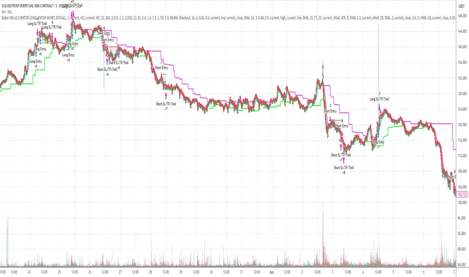
IU Bigger than range strategyDESCRIPTION
IU Bigger Than Range Strategy is designed to capture breakout opportunities by identifying candles that are significantly larger than the previous range. It dynamically calculates the high and low of the last N candles and enters trades when the current candle's range exceeds the previous range. The strategy includes multiple stop-loss methods (Previous High/Low, ATR, Swing High/Low) and automatically manages take-profit and stop-loss levels based on user-defined risk-to-reward ratios. This versatile strategy is optimized for higher timeframes and assets like BTC but can be fine-tuned for different instruments and intervals.
USER INPUTS:
Look back Length: Number of candles to calculate the high-low range. Default is 22.
Risk to Reward: Sets the target reward relative to the stop-loss distance. Default is 3.
Stop Loss Method: Choose between:(Default is "Previous High/Low")
- Previous High/Low
- ATR (Average True Range)
- Swing High/Low
ATR Length: Defines the length for ATR calculation (only applicable when ATR is selected as the stop-loss method) (Default is 14).
ATR Factor: Multiplier applied to the ATR to determine stop-loss distance(Default is 2).
Swing High/Low Length: Specifies the length for identifying swing points (only applicable when Swing High/Low is selected as the stop-loss method).(Default is 2)
LONG CONDITION:
The current candle’s range (absolute difference between open and close) is greater than the previous range.
The closing price is higher than the opening price (bullish candle).
SHORT CONDITIONS:
The current candle’s range exceeds the previous range.
The closing price is lower than the opening price (bearish candle).
LONG EXIT:
Stop-loss:
- Previous Low
- ATR-based trailing stop
- Recent Swing Low
Take-profit:
- Defined by the Risk-to-Reward ratio (default 3x the stop-loss distance).
SHORT EXIT:
Stop-loss:
- Previous High
- ATR-based trailing stop
- Recent Swing High
Take-profit:
- Defined by the Risk-to-Reward ratio (default 3x the stop-loss distance).
ALERTS:
Long Entry Triggered
Short Entry Triggered
WHY IT IS UNIQUE:
This strategy dynamically adapts to different market conditions by identifying candles that exceed the previous range, ensuring that it only enters trades during strong breakout scenarios.
Multiple stop-loss methods provide flexibility for different trading styles and risk profiles.
The visual representation of stop-loss and take-profit levels with color-coded plots improves trade monitoring and decision-making.
HOW USERS CAN BENEFIT FROM IT:
Ideal for breakout traders looking to capitalize on momentum-driven price moves.
Provides flexibility to customize stop-loss methods and fine-tune risk management parameters.
Helps minimize drawdowns with a strong risk-to-reward framework while maximizing profit potential.
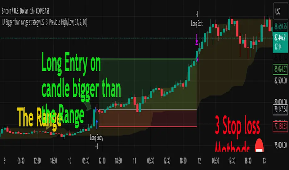
16. SMC Strategy with SL - low TimeframeOverview
The "SMC Strategy with SL - low Timeframe" is a comprehensive trading strategy that uses key concepts from Smart Money Theory to identify favorable areas in the market for buying or selling. This strategy takes advantage of price imbalances, support and resistance zones, and swing highs/lows to generate high-probability trade signals.
The key features of this strategy include:
Swing High/Low Analysis: Used to determine the Premium, Equilibrium, and Discount Zones.
Order Block Integration: An added layer of confluence to identify valid buy and sell signals.
Trend Direction Confirmation: Using a Simple Moving Average (SMA) to determine the overall trend.
Entry and Exit Rules: Based on price position relative to key zones and moving average, along with optional stop-loss and take-profit levels.
Detailed Description
Swing High and Swing Low Analysis
The script calculates Swing High and Swing Low based on the most recent price highs and lows over a specified look-back period (swingHighLength and swingLowLength, set to 8 by default).
It then derives the Premium, Equilibrium, and Discount Zones:
Premium Zone: Represents potential resistance, calculated based on recent swing highs.
Discount Zone: Represents potential support, calculated based on recent swing lows.
Equilibrium: The midpoint between Swing High and Swing Low, dividing the price range into Premium (above equilibrium) and Discount (below equilibrium) areas.
Zone Visualization
The strategy plots the Premium Zone (resistance) in red, the Discount Zone (support) in green, and the Equilibrium level in blue on the chart. This helps visually assess the current price relative to these important areas.
Simple Moving Average (SMA)
A 50-period Simple Moving Average (SMA) is added to help identify the trend direction.
Buy signals are valid only if the price is above the SMA, indicating an uptrend.
Sell signals are valid only if the price is below the SMA, indicating a downtrend.
Entry Rules
The script generates buy or sell signals when certain conditions are met:
A buy signal is triggered when:
Price is below the Equilibrium and within the Discount Zone.
Price is above the SMA.
The buy signal is further confirmed by the presence of an Order Block (recent lowest price area).
A sell signal is triggered when:
Price is above the Equilibrium and within the Premium Zone.
Price is below the SMA.
The sell signal is further confirmed by the presence of an Order Block (recent highest price area).
Order Block
The strategy defines Order Blocks as recent highs and lows within a look-back period (orderBlockLength set to 20 by default).
These blocks represent areas where large players (smart money) have historically been active, increasing the probability of the price reacting in these areas again.
Trade Management and Trade Direction
The user can set Trade Direction to either "Long Only," "Short Only," or "Both." This allows the strategy to adapt based on market conditions or trading preferences.
Based on the Trade Direction, the strategy either:
Closes open trades that are against new signals.
Allows only specific directional trades (either long or short).
Stop-loss levels are defined based on a fixed percentage (stop_loss_percent), which helps to manage risk and minimize losses.
Exit Rules
The strategy uses stop-loss levels for risk management.
A stop-loss price is set at a fixed percentage below the entry price for long positions or above the entry price for short positions.
When the price hits the defined stop-loss level, the trade is closed.
Liquidity Zones
The script identifies recent Swing Highs and Lows as potential liquidity zones. These are levels where price could react strongly, as they represent areas of interest for large traders.
The liquidity zones are plotted as crosses on the chart, marking areas where price may encounter significant buying or selling pressure.
Visual Feedback
The script uses visual markers (green for buy signals and red for sell signals) to indicate potential entries on the chart.
It also plots liquidity zones to help traders identify areas where stop hunts and liquidity grabs might occur.
Monthly Performance Dashboard
The script includes a performance tracking feature that displays monthly profit and loss metrics on the chart.
This dashboard allows the trader to see a visual representation of trading performance over time, providing insights into profitability and consistency.
The table shows profit or loss for each month and year, allowing the user to track the overall success of the strategy.
Key Benefits
Smart Money Concepts (SMC): This strategy incorporates SMC principles like order blocks and liquidity zones, which are used by institutional traders to determine potential market moves.
Zone Analysis: The use of Premium, Discount, and Equilibrium zones provides a solid framework for determining where to enter and exit trades based on price discounts or premiums.
Confluence: Signals are not taken in isolation. They are confirmed by factors like trend direction (SMA) and order blocks, providing greater trade accuracy.
Risk Management: By integrating stop-loss functionality, traders can manage their risks effectively.
Visual Performance Metrics: The monthly and yearly performance dashboard gives valuable feedback on how well the strategy has performed historically.
Practical Use
Buy in Discount Zone: Traders would be looking to buy when the price is discounted relative to its recent range and is above the SMA, indicating an overall uptrend.
Sell in Premium Zone: Conversely, traders would be looking to sell when the price is at a premium relative to its recent range and below the SMA, indicating an overall downtrend.
Order Block Confirmation: Ensures that buying or selling is supported by historical price behavior at significant levels, providing confidence that the market is likely to react at these areas.
This strategy is designed to help traders take advantage of price inefficiencies and areas where institutional traders are likely to be active, increasing the odds of successful trades. By leveraging Smart Money concepts and strong technical confluence, it aims to provide high-probability trade setups.

Superior-Range Bound Renko - Strategy - 11-29-25 - SignalLynxSuperior-Range Bound Renko Strategy with Advanced Risk Management Template
Signal Lynx | Free Scripts supporting Automation for the Night-Shift Nation 🌙
1. Overview
Welcome to Superior-Range Bound Renko (RBR) — a volatility-aware, structure-respecting swing-trading system built on top of a full Risk Management (RM) Template from Signal Lynx.
Instead of relying on static lookbacks (like “14-period RSI”) or plain MA crosses, Superior RBR:
Adapts its range definition to market volatility in real time
Emulates Renko Bricks on a standard, time-based chart (no Renko chart type required)
Uses a stack of Laguerre Filters to detect genuine impulse vs. noise
Adds an Adaptive SuperTrend powered by a small k-means-style clustering routine on volatility
Under the hood, this script also includes the full Signal Lynx Risk Management Engine:
A state machine that separates “Signal” from “Execution”
Layered exit tools: Stop Loss, Trailing Stop, Staged Take Profit, Advanced Adaptive Trailing Stop (AATS), and an RSI-style stop (RSIS)
Designed for non-repainting behavior on closed candles by basing execution-critical logic on previous-bar data
We are publishing this as an open-source template so traders and developers can leverage a professional-grade RM engine while integrating their own signal logic if they wish.
2. Quick Action Guide (TL;DR)
Best Timeframe:
4 Hours (H4) and above. This is a high-conviction swing-trading system, not a scalper.
Best Assets:
Volatile instruments that still respect market structure:
Bitcoin, Ethereum, Gold (XAUUSD), high-volatility Forex pairs (e.g., GBPJPY), indices with clean ranges.
Strategy Type:
Volatility-Adaptive Trend Following + Impulse Detection.
It hunts for genuine expansion out of ranges, not tiny mean-reversion nibbles.
Key Feature:
Renko Emulation on time-based candles.
We mathematically model Renko Bricks and overlay them on your standard chart to define:
“Equilibrium” zones (inside the brick structure)
“Breakout / impulse” zones (when price AND the impulse line depart from the bricks)
Repainting:
Designed to be non-repainting on closed candles.
All RM execution logic uses confirmed historical data (no future bars, no security() lookahead). Intrabar flicker during formation is allowed, but once a bar closes the engine’s decisions are stable.
Core Toggles & Filters:
Enable Longs and Shorts independently
Optional Weekend filter (block trades on Saturday/Sunday)
Per-module toggles: Stop Loss, Trailing Stop, Staged Take Profits, AATS, RSIS
3. Detailed Report: How It Works
A. The Strategy Logic: Superior RBR
Superior RBR builds its entry signal from multiple mathematical layers working together.
1) Adaptive Lookback (Volatility Normalization)
Instead of a fixed 100-bar or 200-bar range, the script:
Computes ATR-based volatility over a user-defined period.
Normalizes that volatility relative to its recent min/max.
Maps the normalized value into a dynamic lookback window between a minimum and maximum (e.g., 4 to 100 bars).
High Volatility:
The lookback shrinks, so the system reacts faster to explosive moves.
Low Volatility:
The lookback expands, so the system sees a “bigger picture” and filters out chop.
All the core “Range High/Low” and “Range Close High/Low” boundaries are built on top of this adaptive window.
2) Range Construction & Quick Ranges
The engine constructs several nested ranges:
Outer Range:
rangeHighFinal – dynamic highest high
rangeLowFinal – dynamic lowest low
Inner Close Range:
rangeCloseHighFinal – highest close
rangeCloseLowFinal – lowest close
Quick Ranges:
“Half-length” variants of those, used to detect more responsive changes in structure and volatility.
These ranges define:
The macro box price is trading inside
Shorter-term “pressure zones” where price is coiling before expansion
3) Renko Emulation (The Bricks)
Rather than using the Renko chart type (which discards time), this script emulates Renko behavior on your normal candles:
A “brick size” is defined either:
As a standard percentage move, or
As a volatility-driven (ATR) brick, optionally inhibited by a minimum standard size
The engine tracks a base value and derives:
brickUpper – top of the emulated brick
brickLower – bottom of the emulated brick
When price moves sufficiently beyond those levels, the brick “shifts”, and the directional memory (renkoDir) updates:
renkoDir = +2 when bricks are advancing upward
renkoDir = -2 when bricks are stepping downward
You can think of this as a synthetic Renko tape overlaid on time-based candles:
Inside the brick: equilibrium / consolidation
Breaking away from the brick: momentum / expansion
4) Impulse Tracking with Laguerre Filters
The script uses multiple Laguerre Filters to smooth price and brick-derived data without traditional lag.
Key filters include:
LagF_1 / LagF_W: Based on brick upper/lower baselines
LagF_Q: Based on HLCC4 (high + low + 2×close)/4
LagF_Y / LagF_P: Complex averages combining brick structures and range averages
LagF_V (Primary Impulse Line):
A smooth, high-level impulse line derived from a blend of the above plus the outer ranges
Conceptually:
When the impulse line pushes away from the brick structure and continues in one direction, an impulse move is underway.
When its direction flips and begins to roll over, the impulse is fading, hinting at mean reversion back into the range.
5) Fib-Based Structure & Swaps
The system also layers in Fib levels derived from the adaptive ranges:
Standard levels (12%, 23.6%, 38.2%, 50%, 61%, 76.8%, 88%) from the main range
A secondary “swap” set derived from close-range dynamics (fib12Swap, fib23Swap, etc.)
These Fibs are used to:
Bucket price into structural zones (below 12, between 23–38, etc.)
Detect breakouts when price and Laguerre move beyond key Fib thresholds
Drive zSwap logic (where a secondary Fib set becomes the active structure once certain conditions are met)
6) Adaptive SuperTrend with K-Means-Style Volatility Clustering
Under the hood, the script uses a small k-means-style clustering routine on ATR:
ATR is measured over a fixed period
The range of ATR values is split into Low, Medium, High volatility centroids
Current ATR is assigned to the nearest centroid (cluster)
From that, a SuperTrend variant (STK) is computed with dynamic sensitivity:
In quiet markets, SuperTrend can afford to be tighter
In wild markets, it widens appropriately to avoid constant whipsaw
This SuperTrend-based oscillator (LagF_K and its signals) is then combined with the brick and Laguerre stack to confirm valid trend regimes.
7) Final Baseline Signals (+2 / -2)
The “brain” of Superior RBR lives in the Baseline & Signal Generation block:
Two composite signals are built: B1 and B2:
They combine:
Fib breakouts
Renko direction (renkoDir)
Expansion direction (expansionQuickDir)
Multiple Laguerre alignments (LagF_Q, LagF_W, LagF_Y, LagF_Z, LagF_P, LagF_V)
They also factor in whether Fib structures are expanding or contracting.
A user toggle selects the “Baseline” signal:
finalSig = B2 (default) or B1 (alternate baseline)
finalSig is then filtered through the RM state machine and only when everything aligns, we emit:
+2 = Long / Buy signal
-2 = Short / Sell signal
0 = No new trade
Those +2 / -2 values are what feed the Risk Management Engine.
B. The Risk Management (RM) Engine
This script features the Signal Lynx Risk Management Engine, a proprietary state machine built to separate Signal from Execution.
Instead of firing orders directly on indicator conditions, we:
Convert the raw signal into a clean integer (Fin = +2 / -2 / 0)
Feed it into a Trade State Machine that understands:
Are we flat?
Are we in a long or short?
Are we in a closing sequence?
Should we permit re-entry now or wait?
Logic Injection / Template Concept:
The RM engine expects a simple integer:
+2 → Buy
-2 → Sell
Everything else (0) is “no new trade”
This makes the script a template:
You can remove the Superior RBR block
Drop in your own logic (RSI, MACD, price action, etc.)
As long as you output +2 or -2 into the same signal channel, the RM engine can drive all exits and state transitions.
Aggressive vs Conservative Modes:
The input AgressiveRM (Aggressive RM) governs how we interpret signals:
Conservative Mode (Aggressive RM = false):
Uses a more filtered internal signal (AF) to open trades
Effectively waits for a clean trend flip / confirmation before new entries
Minimizes whipsaw at the cost of fewer trades
Aggressive Mode (Aggressive RM = true):
Reacts directly to the fresh alert (AO) pulses
Allows faster re-entries in the same direction after RM-based exits
Still respects your pyramiding setting; this script ships with pyramiding = 0 by default, so it will not stack multiple positions unless you change that parameter in the strategy() call.
The state machine enforces discipline on top of your signal logic, reducing double-fires and signal spam.
C. Advanced Exit Protocols (Layered Defense)
The exit side is where this template really shines. Instead of a single “take profit or stop loss,” it uses multiple, cooperating layers.
1) Hard Stop Loss
A classic percentage-based Stop Loss (SL) relative to the entry price.
Acts as a final “catastrophic protection” layer for unexpected moves.
2) Standard Trailing Stop
A percentage-based Trailing Stop (TS) that:
Activates only after price has moved a certain percentage in your favor (tsActivation)
Then trails price by a configurable percentage (ts)
This is a straightforward, battle-tested trailing mechanism.
3) Staged Take Profits (Three Levels)
The script supports three staged Take Profit levels (TP1, TP2, TP3):
Each stage has:
Activation percentage (how far price must move in your favor)
Trailing amount for that stage
Position percentage to close
Example setup:
TP1:
Activate at +10%
Trailing 5%
Close 10% of the position
TP2:
Activate at +20%
Trailing 10%
Close another 10%
TP3:
Activate at +30%
Trailing 5%
Close the remaining 80% (“runner”)
You can tailor these quantities for partial scaling out vs. letting a core position ride.
4) Advanced Adaptive Trailing Stop (AATS)
AATS is a sophisticated volatility- and structure-aware stop:
Uses Hirashima Sugita style levels (HSRS) to model “floors” and “ceilings” of price:
Dungeon → Lower floors → Mid → Upper floors → Penthouse
These levels classify where current price sits within a long-term distribution.
Combines HSRS with Bollinger-style envelopes and EMAs to determine:
Is price extended far into the upper structure?
Is it compressed near the lower ranges?
From this, it computes an adaptive factor that controls how tight or loose the trailing level (aATS / bATS) should be:
High Volatility / Penthouse areas:
Stop loosens to avoid getting wicked out by inevitable spikes.
Low Volatility / compressed structure:
Stop tightens to lock in and protect profit.
AATS is designed to be the “smart last line” that responds to context instead of a single fixed percentage.
5) RSI-Style Stop (RSIS)
On top of AATS, the script includes a RSI-like regime filter:
A McGinley Dynamic mean of price plus ATR bands creates a dynamic channel.
Crosses above the top band and below the lower band change a directional state.
When enabled (UseRSIS):
RSIS can confirm or veto AATS closes:
For longs: A shift to bearish RSIS can force exits sooner.
For shorts: A shift to bullish RSIS can do the same.
This extra layer helps avoid over-reactive stops in strong trends while still respecting a regime change when it happens.
D. Repainting Protection
Many strategies look incredible in the Strategy Tester but fail in live trading because they rely on intrabar values or future-knowledge functions.
This template is built with closed-candle realism in mind:
The Risk Management logic explicitly uses previous bar data (open , high , low , close ) for the key decisions on:
Trailing stop updates
TP triggers
SL hits
RM state transitions
No security() lookahead or future-bar access is used.
This means:
Backtest behavior is designed to match what you can actually get with TradingView alerts and live automation.
Signals may “flicker” intrabar while the candle is forming (as with any strategy), but on closed candles, the RM decisions are stable and non-repainting.
4. For Developers & Modders
We strongly encourage you to mod this script.
To plug your own strategy into the RM engine:
Look for the section titled:
// BASELINE & SIGNAL GENERATION
You will see composite logic building B1 and B2, and then selecting:
baseSig = B2
altSig = B1
finalSig = sigSwap ? baseSig : altSig
You can replace the content used to generate baseSig / altSig with your own logic, for example:
RSI crosses
MACD histogram flips
Candle pattern detectors
External condition flags
Requirements are simple:
Your final logic must output:
2 → Buy signal
-2 → Sell signal
0 → No new trade
That output flows into the RM engine via finalSig → AlertOpen → state machine → Fin.
Once you wire your signals into finalSig, the entire Risk Management system (Stops, TPs, AATS, RSIS, re-entry logic, weekend filters, long/short toggles) becomes available for your custom strategy without re-inventing the wheel.
This makes Superior RBR not just a strategy, but a reference architecture for serious Pine dev work.
5. About Signal Lynx
Automation for the Night-Shift Nation 🌙
Signal Lynx focuses on helping traders and developers bridge the gap between indicator logic and real-world automation. The same RM engine you see here powers multiple internal systems and templates, including other public scripts like the Super-AO Strategy with Advanced Risk Management.
We provide this code open source under the Mozilla Public License 2.0 (MPL-2.0) to:
Demonstrate how Adaptive Logic and structured Risk Management can outperform static, one-layer indicators
Give Pine Script users a battle-tested RM backbone they can reuse, remix, and extend
If you are looking to automate your TradingView strategies, route signals to exchanges, or simply want safer, smarter strategy structures, please keep Signal Lynx in your search.
License: Mozilla Public License 2.0 (Open Source).
If you make beneficial modifications, please consider releasing them back to the community so everyone can benefit.

ICT Liquidity Sweep Asia/London 1 Trade per High & Low🧠 ICT Liquidity Sweep Asia/London — 1 Trade per High & Low
This strategy is inspired by the ICT (Inner Circle Trader) concepts of liquidity sweeps and market structure, focusing on the Asia and London sessions.
It automatically identifies liquidity grabs (sweeps) above or below key session highs/lows and enters trades with a fixed risk/reward ratio (RR).
----------------------------------------------------------------------------------
----------------------------------------------------------------------------------
⚙️ Core Logic
-Asia Session: 8:00 PM – 11:59 PM (New York time)
-London Session: 2:00 AM – 5:00 AM (New York time)
-The script marks the Asia High/Low and London High/Low ranges for each day.
-When the market sweeps above a session high → potential Short setup
-When the market sweeps below a session low → potential Long setup
-A trade is triggered when the confirmation candle closes in the opposite direction of the sweep (bearish after a high sweep, bullish after a low sweep).
-Only one trade per sweep type (1 per High, 1 per Low) is allowed per session.
----------------------------------------------------------------------------------
----------------------------------------------------------------------------------
📈 Risk Management
-Configurable Risk/Reward Target (default = 2:1)
-Configurable Position Size (number of contracts)
-Each trade uses a fixed Stop Loss (beyond the wick of the sweep) and a Take Profit calculated from the RR setting.
-All trades are automatically logged in the Strategy Tester with performance metrics.
----------------------------------------------------------------------------------
----------------------------------------------------------------------------------
💡 Features
✅ Visual session highlighting (Asia = Aqua, London = Orange)
✅ Automatic liquidity line plotting (session highs/lows)
✅ Entry & exit labels (optional visual display)
✅ Customizable RR and contract size
✅ Works on any instrument (ideal for indices, futures, or forex)
✅ Compatible with all timeframes (optimized for 1M–15M)
----------------------------------------------------------------------------------
----------------------------------------------------------------------------------
⚠️ Notes
-Best used on New York time-based charts.
-Designed for educational and backtesting purposes — not financial advice.
-Use as a foundation for further optimization (e.g., SMT confirmation, FVG filter, or time-based restrictions).
----------------------------------------------------------------------------------
----------------------------------------------------------------------------------
🧩 Recommended Use
Pair this with:
-ICT’s concepts like CISD (Change in State of Delivery) and FVGs (Fair Value Gaps)
-Higher timeframe liquidity maps
-Session bias or daily narrative filters
----------------------------------------------------------------------------------
----------------------------------------------------------------------------------
Author: jygirouard
Strategy Version: 1.3
Type: ICT Liquidity Sweep Automation
Timezone: America/New_York
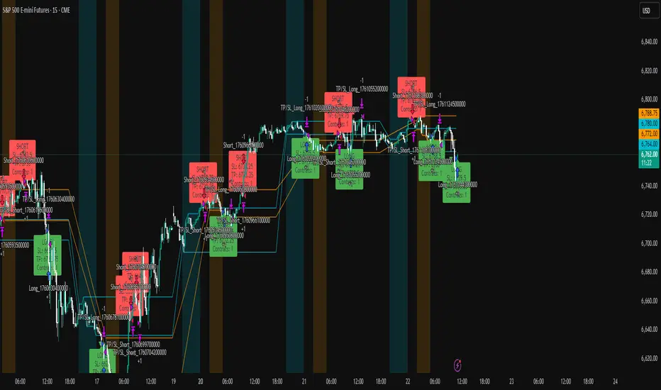
Bullish Reversal Bar Strategy [Skyrexio]Overview
Bullish Reversal Bar Strategy leverages the combination of candlestick pattern Bullish Reversal Bar (description in Methodology and Justification of Methodology), Williams Alligator indicator and Williams Fractals to create the high probability setups. Candlestick pattern is used for the entering into trade, while the combination of Williams Alligator and Fractals is used for the trend approximation as close condition. Strategy uses only long trades.
Unique Features
No fixed stop-loss and take profit: Instead of fixed stop-loss level strategy utilizes technical condition obtained by Fractals and Alligator or the candlestick pattern invalidation to identify when current uptrend is likely to be over (more information in "Methodology" and "Justification of Methodology" paragraphs)
Configurable Trading Periods: Users can tailor the strategy to specific market windows, adapting to different market conditions.
Trend Trade Filter: strategy uses Alligator and Fractal combination as high probability trend filter.
Methodology
The strategy opens long trade when the following price met the conditions:
1.Current candle's high shall be below the Williams Alligator's lines (Jaw, Lips, Teeth)(all details in "Justification of Methodology" paragraph)
2.Price shall create the candlestick pattern "Bullish Reversal Bar". Optionally if MFI and AO filters are enabled current candle shall have the decreasing AO and at least one of three recent bars shall have the squat state on the MFI (all details in "Justification of Methodology" paragraph)
3.If price breaks through the high of the candle marked as the "Bullish Reversal Bar" the long trade is open at the price one tick above the candle's high
4.Initial stop loss is placed at the Bullish Reversal Bar's candle's low
5.If price hit the Bullish Reversal Bar's low before hitting the entry price potential trade is cancelled
6.If trade is active and initial stop loss has not been hit, trade is closed when the combination of Alligator and Williams Fractals shall consider current trend change from upward to downward.
Strategy settings
In the inputs window user can setup strategy setting:
Enable MFI (if true trades are filtered using Market Facilitation Index (MFI) condition all details in "Justification of Methodology" paragraph), by default = false)
Enable AO (if true trades are filtered using Awesome Oscillator (AO) condition all details in "Justification of Methodology" paragraph), by default = false)
Justification of Methodology
Let's explore the key concepts of this strategy and understand how they work together. The first and key concept is the Bullish Reversal Bar candlestick pattern. This is just the single bar pattern. The rules are simple:
Candle shall be closed in it's upper half
High of this candle shall be below all three Alligator's lines (Jaw, Lips, Teeth)
Next, let’s discuss the short-term trend filter, which combines the Williams Alligator and Williams Fractals. Williams Alligator
Developed by Bill Williams, the Alligator is a technical indicator that identifies trends and potential market reversals. It consists of three smoothed moving averages:
Jaw (Blue Line): The slowest of the three, based on a 13-period smoothed moving average shifted 8 bars ahead.
Teeth (Red Line): The medium-speed line, derived from an 8-period smoothed moving average shifted 5 bars forward.
Lips (Green Line): The fastest line, calculated using a 5-period smoothed moving average shifted 3 bars forward.
When the lines diverge and align in order, the "Alligator" is "awake," signaling a strong trend. When the lines overlap or intertwine, the "Alligator" is "asleep," indicating a range-bound or sideways market. This indicator helps traders determine when to enter or avoid trades.
Fractals, another tool by Bill Williams, help identify potential reversal points on a price chart. A fractal forms over at least five consecutive bars, with the middle bar showing either:
Up Fractal: Occurs when the middle bar has a higher high than the two preceding and two following bars, suggesting a potential downward reversal.
Down Fractal: Happens when the middle bar shows a lower low than the surrounding two bars, hinting at a possible upward reversal.
Traders often use fractals alongside other indicators to confirm trends or reversals, enhancing decision-making accuracy.
How do these tools work together in this strategy? Let’s consider an example of an uptrend.
When the price breaks above an up fractal, it signals a potential bullish trend. This occurs because the up fractal represents a shift in market behavior, where a temporary high was formed due to selling pressure. If the price revisits this level and breaks through, it suggests the market sentiment has turned bullish.
The breakout must occur above the Alligator’s teeth line to confirm the trend. A breakout below the teeth is considered invalid, and the downtrend might still persist. Conversely, in a downtrend, the same logic applies with down fractals.
How we can use all these indicators in this strategy? This strategy is a counter trend one. Candle's high shall be below all Alligator's lines. During this market stage the bullish reversal bar candlestick pattern shall be printed. This bar during the downtrend is a high probability setup for the potential reversal to the upside: bulls were able to close the price in the upper half of a candle. The breaking of its high is a high probability signal that trend change is confirmed and script opens long trade. If market continues going down and break down the bullish reversal bar's low potential trend change has been invalidated and strategy close long trade.
If market really reversed and started moving to the upside strategy waits for the trend change form the downtrend to the uptrend according to approximation of Alligator and Fractals combination. If this change happens strategy close the trade. This approach helps to stay in the long trade while the uptrend continuation is likely and close it if there is a high probability of the uptrend finish.
Optionally users can enable MFI and AO filters. First of all, let's briefly explain what are these two indicators. The Awesome Oscillator (AO), created by Bill Williams, is a momentum-based indicator that evaluates market momentum by comparing recent price activity to a broader historical context. It assists traders in identifying potential trend reversals and gauging trend strength.
AO = SMA5(Median Price) − SMA34(Median Price)
where:
Median Price = (High + Low) / 2
SMA5 = 5-period Simple Moving Average of the Median Price
SMA 34 = 34-period Simple Moving Average of the Median Price
This indicator is filtering signals in the following way: if current AO bar is decreasing this candle can be interpreted as a bullish reversal bar. This logic is applicable because initially this strategy is a trend reversal, it is searching for the high probability setup against the current trend. Decreasing AO is the additional high probability filter of a downtrend.
Let's briefly look what is MFI. The Market Facilitation Index (MFI) is a technical indicator that measures the price movement per unit of volume, helping traders gauge the efficiency of price movement in relation to trading volume. Here's how you can calculate it:
MFI = (High−Low)/Volume
MFI can be used in combination with volume, so we can divide 4 states. Bill Williams introduced these to help traders interpret the interaction between volume and price movement. Here’s a quick summary:
Green Window (Increased MFI & Increased Volume): Indicates strong momentum with both price and volume increasing. Often a sign of trend continuation, as both buying and selling interest are rising.
Fake Window (Increased MFI & Decreased Volume): Shows that price is moving but with lower volume, suggesting weak support for the trend. This can signal a potential end of the current trend.
Squat Window (Decreased MFI & Increased Volume): Shows high volume but little price movement, indicating a tug-of-war between buyers and sellers. This often precedes a breakout as the pressure builds.
Fade Window (Decreased MFI & Decreased Volume): Indicates a lack of interest from both buyers and sellers, leading to lower momentum. This typically happens in range-bound markets and may signal consolidation before a new move.
For our purposes we are interested in squat bars. This is the sign that volume cannot move the price easily. This type of bar increases the probability of trend reversal. In this indicator we added to enable the MFI filter of reversal bars. If potential reversal bar or two preceding bars have squat state this bar can be interpret as a reversal one.
Backtest Results
Operating window: Date range of backtests is 2023.01.01 - 2024.12.31. It is chosen to let the strategy to close all opened positions.
Commission and Slippage: Includes a standard Binance commission of 0.1% and accounts for possible slippage over 5 ticks.
Initial capital: 10000 USDT
Percent of capital used in every trade: 50%
Maximum Single Position Loss: -5.29%
Maximum Single Profit: +29.99%
Net Profit: +5472.66 USDT (+54.73%)
Total Trades: 103 (33.98% win rate)
Profit Factor: 1.634
Maximum Accumulated Loss: 1231.15 USDT (-8.32%)
Average Profit per Trade: 53.13 USDT (+0.94%)
Average Trade Duration: 76 hours
How to Use
Add the script to favorites for easy access.
Apply to the desired timeframe and chart (optimal performance observed on 4h ETH/USDT).
Configure settings using the dropdown choice list in the built-in menu.
Set up alerts to automate strategy positions through web hook with the text: {{strategy.order.alert_message}}
Disclaimer:
Educational and informational tool reflecting Skyrex commitment to informed trading. Past performance does not guarantee future results. Test strategies in a simulated environment before live implementation
These results are obtained with realistic parameters representing trading conditions observed at major exchanges such as Binance and with realistic trading portfolio usage parameters.

Octopus Nest Strategy Hello Fellas,
Hereby, I come up with a popular strategy from YouTube called Octopus Nest Strategy. It is a no repaint, lower timeframe scalping strategy utilizing PSAR, EMA and TTM Squeeze.
The strategy considers these market factors:
PSAR -> Trend
EMA -> Trend
TTM Squeeze -> Momentum and Volatility by incorporating Bollinger Bands and Keltner Channels
Note: As you can see there is a potential improvement by incorporating volume.
What's Different Compared To The Original Strategy?
I added an option which allows users to use the Adaptive PSAR of @loxx, which will hopefully improve results sometimes.
Signals
Enter Long -> source above EMA 100, source crosses above PSAR and TTM Squeeze crosses above 0
Enter Short -> source below EMA 100, source crosses below PSAR and TTM Squeeze crosses below 0
Exit Long and Exit Short are triggered from the risk management. Thus, it will just exit on SL or TP.
Risk Management
"High Low Stop Loss" and "Automatic High Low Take Profit" are used here.
High Low Stop Loss: Utilizes the last high for short and the last low for long to calculate the stop loss level. The last high or low gets multiplied by the user-defined multiplicator and if no recent high or low was found it uses the backup multiplier.
Automatic High Low Take Profit: Utilizes the current stop loss level of "High Low Stop Loss" and gets calculated by the user-defined risk ratio.
Now, follows the bunch of knowledge for the more inexperienced readers.
PSAR: Parabolic Stop And Reverse; Developed by J. Welles Wilders and a classic trend reversal indicator.
The indicator works most effectively in trending markets where large price moves allow traders to capture significant gains. When a security’s price is range-bound, the indicator will constantly be reversing, resulting in multiple low-profit or losing trades.
TTM Squeeze: TTM Squeeze is a volatility and momentum indicator introduced by John Carter of Trade the Markets (now Simpler Trading), which capitalizes on the tendency for price to break out strongly after consolidating in a tight trading range.
The volatility component of the TTM Squeeze indicator measures price compression using Bollinger Bands and Keltner Channels. If the Bollinger Bands are completely enclosed within the Keltner Channels, that indicates a period of very low volatility. This state is known as the squeeze. When the Bollinger Bands expand and move back outside of the Keltner Channel, the squeeze is said to have “fired”: volatility increases and prices are likely to break out of that tight trading range in one direction or the other. The on/off state of the squeeze is shown with small dots on the zero line of the indicator: red dots indicate the squeeze is on, and green dots indicate the squeeze is off.
EMA: Exponential Moving Average; Like a simple moving average, but with exponential weighting of the input data.
Don't forget to check out the settings and keep it up.
Best regards,
simwai
---
Credits to:
@loxx
@Bjorgum
@Greeny
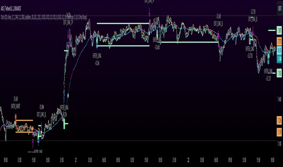
YinYang RSI Volume Trend StrategyThere are many strategies that use RSI or Volume but very few that take advantage of how useful and important the two of them combined are. This strategy uses the Highs and Lows with Volume and RSI weighted calculations on top of them. You may be wondering how much of an impact Volume and RSI can have on the prices; the answer is a lot and we will discuss those with plenty of examples below, but first…
How does this strategy work?
It’s simple really, when the purchase source crosses above the inner low band (red) it creates a Buy or Long. This long has a Trailing Stop Loss band (the outer low band that's also red) that can be adjusted in the Settings. The Stop Loss is based on a % of the inner low band’s price and by default it is 0.1% lower than the inner band’s price. This Stop Loss is not only a stop loss but it can also act as a Purchase Available location.
You can get back into a trade after a stop loss / take profit has been hit when your Reset Purchase Availability After condition has been met. This can either be at Stop Loss, Entry or None.
It is advised to allow it to reset in case the stop loss was a fake out but the call was right. Sometimes it may trigger stop loss multiple times in a row, but you don’t lose much on stop loss and you gain lots when the call is right.
The Take Profit location is the basis line (white). Take Profit occurs when the Exit Source (close, open, high, low or other) crosses the basis line and then on a different bar the Exit Source crosses back over the basis line. For example, if it was a Long and the bar’s Exit Source closed above the basis line, and then 2 bars later its Exit Source closed below the basis line, Take Profit would occur. You can disable Take Profit in Settings, but it is very useful as many times the price will cross the Basis and then correct back rather than making it all the way to the opposing zone.
Longs:
If for instance your Long doesn’t need to Take Profit and instead reaches the top zone, it will close the position when it crosses above the inner top line (green).
Please note you can change the Exit Source too which is what source (close, open, high, low) it uses to end the trades.
The Shorts work the same way as the Long but just opposite, they start when the purchase source crosses under the inner upper band (green).
Shorts:
Shorts take profit when it crosses under the basis line and then crosses back.
Shorts will Stop loss when their outer upper band (green) is crossed with the Exit Source.
Short trades are completed and closed when its Exit Source crosses under the inner low red band.
So, now that you understand how the strategy works, let’s discuss why this strategy works and how it is profitable.
First we will discuss Volume as we deem it plays a much bigger role overall and in our strategy:
As I’m sure many of you know, Volume plays a huge factor in how much something moves, but it also plays a role in the strength of the movement. For instance, let’s look at two scenarios:
Bitcoin’s price goes up $1000 in 1 Day but the Volume was only 10 million
Bitcoin’s price goes up $200 in 1 Day but the Volume was 40 million
If you were to only look at the price, you’d say #1 was more important because the price moved x5 the amount as #2, but once you factor in the volume, you know this is not true. The reason why Volume plays such a huge role in Price movement is because it shows there is a large Limit Order battle going on. It means that both Bears and Bulls believe that price is a good time to Buy and Sell. This creates a strong Support and Resistance price point in this location. If we look at scenario #2, when there is high volume, especially if it is drastically larger than the average volume Bitcoin was displaying recently, what can we decipher from this? Well, the biggest take away is that the Bull’s won the battle, and that likely when that happens we will see bullish movement continuing to happen as most of the Bears Limit Orders have been fulfilled. Whereas with #2, when large price movement happens and Bitcoin goes up $1000 with low volume what can we deduce? The main takeaway is that Bull’s pressured the price up with Market Orders where they purchased the best available price, also what this means is there were very few people who were wanting to sell. This generally dictates that Whale Limit orders for Sells/Shorts are much higher up and theres room for movement, but it also means there is likely a whale that is ready to dump and crash it back down.
You may be wondering, what did this example have to do with YinYang RSI Volume Trend Strategy? Well the reason we’ve discussed this is because we use Volume multiple times to apply multiplications in our calculations to add large weight to the price when there is lots of volume (this is applied both positively and negatively). For instance, if the price drops a little and there is high volume, our strategy will move its bounds MUCH lower than the price actually dropped, and if there was low volume but the price dropped A LOT, our strategy will only move its bounds a little. We believe this reflects higher levels of price accuracy than just price alone based on the examples described above.
Don’t believe us?
Here is with Volume NOT factored in (VWMA = SMA and we remove our Volume Filter calculation):
Which produced -$2880 Profit
Here is with our Volume factored in:
Which produced $553,000 (55.3%)
As you can see, we wen’t from $-2800 profit with volume not factored to $553,000 with volume factored. That's quite a big difference! (Please note previous success does not predict future success we are simply displaying the $ amounts as example).
Now how about RSI and why does it matter in this strategy?
As I’m sure most of you are aware, RSI is one of the leading indicators used in trading. For this reason we figured it would only make sense to incorporate it into our calculations. We fiddled with RSI for quite awhile and sometimes what logically seems to be the right way to use it isn’t. Now, because of this, our RSI calculation is a little odd, but basically what we’re doing is we calculate the RSI, then turn it into a percentage (between 0-1) that can easily be multiplied to the price point we need. The price point we use is the difference between our high purchase zone and our low purchase zone. This allows us to see how much price movement there is between zones. We multiply our zone size with our RSI multiplication and we get the amount we will add +/- to our basis line (white line). This officially creates the NEW high and low purchase zones that we are actually using and displaying in our trades.
If you found that confusing, here are some examples to why it is an important calculation for this strategy:
Before RSI factored in:
Which produced 27.8% Profit
After RSI factored in:
Which produced 553% Profit
As you can see, the RSI makes not only the purchase zones more accurate, but it also greatly increases the profit the strategy is able to make. It also helps ensure an relatively linear profit slope so you know it is reliable with its trades.
This strategy can work on pretty much anything, but you should tweak the values a bit for each pair you are trading it with for best results.
We hope you can find some use out of this simple but effective strategy, if you have any questions, comments or concerns please let us know.
HAPPY TRADING!
Pressure Pivots - MPI (Strategy)⇋ PRESSURE PIVOTS — MARKET PRESSURE INDEX STRATEGY
A comprehensive reversal trading system that combines order flow pressure analysis, multi-factor confluence detection, and adaptive machine learning to identify high-probability turning points in liquid markets.
━━━━━━━━━━━━━━━━━━━━━━━━━━━━━━━━━━━━━
CORE INNOVATION: MARKET PRESSURE INDEX (MPI)
Traditional indicators measure price movement. The Market Pressure Index measures the force behind the movement.
How MPI Works:
Every bar tells two stories through volume distribution:
• Buy Pressure: Volume × (Close - Low) / (High - Low)
• Sell Pressure: Volume × (High - Close) / (High - Low)
• Net Pressure: Buy Pressure - Sell Pressure
This raw pressure is then normalized against baseline activity to create the bounded MPI (-1.0 to +1.0):
• Smooth Pressure: EMA(Net Pressure, period)
• Baseline Activity: SMA(|Net Pressure|, period × 2)
• MPI: (Smooth Pressure / Baseline) × Sensitivity
What MPI Reveals:
MPI > +0.7: Extreme buy pressure → Exhaustion potential
MPI = +0.2 to +0.7: Healthy bullish momentum
MPI = -0.2 to +0.2: Neutral/balanced pressure
MPI = -0.7 to -0.2: Healthy bearish momentum
MPI < -0.7: Extreme sell pressure → Exhaustion potential
Why It Works:
Two bars can both move 10 points, but if one closes at the high on high volume (aggressive buying) and the other closes mid-range on average volume (weak buying), only MPI distinguishes between sustainable momentum and exhaustion. This volume-weighted pressure analysis reveals conviction behind price moves—the key to timing reversals.
━━━━━━━━━━━━━━━━━━━━━━━━━━━━━━━━━━━━━
SEVEN-FACTOR CONFLUENCE SYSTEM
MPI extremes alone aren't enough. The system requires multiple independent confirmations through weighted scoring:
1. DIVERGENCE (Weight: 3.0) — Premium Signal Type: DIV
Price makes new high but MPI makes lower high (or inverse for bullish)
• Detection: Tracks pivots with 5-bar lookback, compares price vs MPI at pivot points
• Signal: Purple triangles, highest weight (pressure weakening while price extends)
2. LIQUIDITY SWEEP (Weight: 2.5) — Premium Signal Type: LIQ
Price breaks swing high/low within 0.3 ATR then reverses
• Detection: Break within tolerance + close back through level
• Signal: Orange triangles, second-highest weight (stop hunt reversal)
3. ORDER FLOW IMBALANCE (Weight: 2.0) — Premium Signal Type: OF
Aggressive buying/selling 50% above normal
• Detection: EMA(aggressive volume) vs SMA(imbalance) threshold
• Signal: Aqua triangles, institutional positioning
4. VELOCITY EXHAUSTION (Weight: 1.5)
Parabolic move (2+ ATRs in 3 bars) + extreme MPI
• Detection: |3-bar price change / ATR| > threshold + MPI > ±0.5
• Indicates: Momentum deceleration, blow-off top/bottom
5. WICK REJECTION (Weight: 1.5)
Single bar: wick > 60% of range, or sequence: 2 bars with 40% + 30% wicks
• Detection: Shooting stars (bearish) or hammers (bullish)
• Indicates: Intrabar rejection, battle won by opposing side
6. VOLUME SPIKE (Weight: 1.0)
Volume > 20-bar average × multiplier (default: 2.0x)
• Detection: Participation surge confirmation
• Lowest weight: Can be manipulated, better as confirmation
7. POSITION FACTOR (Weight: 1.0)
At 10-bar highest (bearish) or lowest (bullish)
• Detection: Structural positioning for reversal
• Base requirement: Must be at extreme to score
Scoring Logic:
Premium Signals (DIV/LIQ/OF): Must score ≥6.0 (default premiumThreshold)
Standard Signals (STD): Must score ≥4.0 (default standardThreshold)
Example Scoring:
Divergence (3.0) + Liquidity Sweep (2.5) + Volume (1.0) = 6.5 → FIRES (DIV signal)
Recent High (1.0) + Wick (1.5) + Volume (1.0) + Velocity (1.5) = 5.0 → FIRES (STD signal)
━━━━━━━━━━━━━━━━━━━━━━━━━━━━━━━━━━━━━
ADAPTIVE LEARNING ENGINE
Unlike static strategies, this system learns from every trade and optimizes itself.
Performance Tracking:
Every trade records:
• Entry Score: Confluence level at entry
• Signal Type: DIV / LIQ / OF / STD
• Win/Loss: Boolean outcome
• R-Multiple: (Exit - Entry) / (Entry - Stop)
• MAE: Maximum Adverse Excursion (worst drawdown)
• MFE: Maximum Favorable Excursion (best profit reached)
Three Adaptive Parameters:
1. Signal Threshold Adaptation
If Win Rate < Target (45%): RAISE threshold → fewer signals, better quality
If Win Rate > Target + 10% AND good R: LOWER threshold → more signals, profitable
2. Stop Distance Adaptation
If Avg MAE > 0.85 AND WR < 50%: WIDEN stops → reduce premature exits
If Avg MAE < 0.4 AND WR > 55%: TIGHTEN stops → reduce risk
3. Target Distance Adaptation
If Avg MFE > Target × 1.5: EXTEND targets → capture more of runners
If Avg MFE < Target × 0.7: SHORTEN targets → take profits faster
Signal Type Filtering:
The system tracks performance by type (DIV/LIQ/OF/STD):
• If Type WR < 40% AND Avg R < 0.8: Type DISABLED
• If Type WR ≥ 40% OR Avg R ≥ 0.8: Type RE-ENABLED
Example: If OF signals consistently lose while DIV signals win, system automatically stops taking OF signals and focuses on DIV.
Warmup Period:
First 30 trades (default) gather baseline data with relaxed thresholds. After warmup, full adaptation activates.
━━━━━━━━━━━━━━━━━━━━━━━━━━━━━━━━━━━━━
COMPLETE POSITION MANAGEMENT
Dynamic Position Sizing:
Base Contracts = (Equity × Risk%) / (Stop Distance × Point Value)
Then multiplied by:
• Score Bonus: Up to +50% for highest-scoring signals
• Signal Type Bonus: DIV signals +50%, LIQ signals +30%
• Streak Multiplier: After 3 losses: 50% reduction, After 3 wins: 25% increase
Example: High-scoring DIV signal on winning streak = 3-4× larger position than weak STD signal on losing streak
Entry Modes:
Single Entry: Full size at once, exit at TP2 (or partial at TP1)
Tiered Entry: 40% at TP1 (2R), 60% at TP2 (4R adaptive)
Stop Management (3 Modes):
Structural: Beyond recent 20-bar swing high/low + buffer
ATR: Fixed ATR multiplier (default: 2.0 ATR, then adapts)
Hybrid: Attempt structural, fallback to ATR if invalid
Plus:
• Breakeven: Move stop to entry ± 1 tick when 1R reached
• Trailing: Activate when 1.5R reached, trail 0.8R behind price
• Max Loss Override: Cap dollar risk regardless of calculation
Target Management:
Fixed Mode: TP1 = 2R, TP2 = 4R
Adaptive Mode: TP1 = 2R fixed, TP2 adapts based on MFE analysis
Partial Exits: Default 50% at TP1, remainder at TP2 or trailing stop
━━━━━━━━━━━━━━━━━━━━━━━━━━━━━━━━━━━━━
COMPREHENSIVE RISK CONTROLS
Daily Limits:
• Max Daily Loss: $2,000 default → HALT trading
• Max Daily Trades: 15 default → prevent overtrading
• Max Concurrent: 2 positions → limit correlation risk
Session Controls:
• Trading Hours: Specify start/end times + timezone
• Weekend Block: Optional (avoid crypto weekend volatility)
Prop Firm Protection (Live Trading Only):
• Daily Loss Limit: Stricter of general or prop limit ($1,000 default)
• Trailing Drawdown: Tracks high water mark, HALTS if breach ($2,500 default)
• Reset on Reload: Optional high water mark reset
Liquidity Filter (Optional):
• Time-Based: Avoid first/last X minutes of session
• Volume-Based: Require minimum volume ratio (0.5× average default)
Market Regime Filter (Optional):
• ADX-Based: Only trade when ADX > threshold (trending)
• Block: Consolidation (ADX < 20) or Transitional regimes
━━━━━━━━━━━━━━━━━━━━━━━━━━━━━━━━━━━━━
REAL-TIME DASHBOARD
MPI Gauge Section:
Shows current pressure: 🟢 STRONG BUY (+0.5 to +1.0), 🟩 BUY PRESSURE (+0.2 to +0.5), ⚪ NEUTRAL (-0.2 to +0.2), 🟥 SELL PRESSURE (-0.5 to -0.2), 🔴 STRONG SELL (-1.0 to -0.5)
Signal Status Section:
• Active Signals: "🔴 DIV SELL" (purple background), "🟢 LIQ BUY" (orange), "🔵 OF SELL" (aqua), "🟢 STD BUY" (green)
• Warnings: "⚠️ BEAR WARNING" / "⚠️ BULL WARNING" (yellow) — setup forming, not full signal
• Scanning: "⏳ SCANNING..." (gray) — no signal active
• Confidence Bar: Visual score display "██████░░░░" showing confluence strength
Divergence Indicator:
"🟣 BEARISH DIVERGENCE" or "🟡 BULLISH DIVERGENCE" when detected
Performance Statistics:
• Overall Win Rate: Wins/Total with visual bar (lime ≥70%, yellow 50-70%, red <50%)
• Directional: Bearish vs Bullish win rates separately
• By Signal Type: DIV / LIQ / OF / STD individual performance tracking
━━━━━━━━━━━━━━━━━━━━━━━━━━━━━━━━━━━━━
KEY PARAMETERS EXPLAINED
🎯 Pressure Engine:
• MPI Period (5-50, default: 14): Smoothing period — lower for scalping, higher for position trading
• MPI Sensitivity (0.5-5.0, default: 1.5): Amplification — lower compresses range, higher more extremes
🔍 Detection:
• Wick Threshold (0.3-0.9, default: 0.6): Minimum wick-to-range ratio for rejection
• Volume Spike (1.2-3.0x, default: 2.0): Multiplier above average for spike
• Aggressive Ratio (0.5-0.9, default: 0.65): Close position in range for aggressive orders
• Velocity Threshold (1.0-5.0 ATR, default: 2.0): ATR-normalized move for exhaustion
• MPI Extreme (0.5-0.95, default: 0.7): Level considered overbought/oversold
⚖️ Weights:
• Divergence: 3.0 (highest — pressure weakening)
• Liquidity: 2.5 (second — stop hunts)
• Order Flow: 2.0 (institutional positioning)
• Velocity: 1.5 (momentum exhaustion)
• Wick: 1.5 (rejection patterns)
• Volume: 1.0 (lowest — can be manipulated)
🎚️ Thresholds:
• Premium (4.0-15.0, default: 6.0): Score for DIV/LIQ/OF signals
• Standard (2.0-8.0, default: 4.0): Score for STD signals
• Warning Confluence (1-4, default: 2): Factors for yellow diamond warnings
🧬 Adaptive:
• Enable (true/false, default: true): Master learning switch
• Warmup Trades (5-100, default: 30): Data collection before adaptation
• Lookback (20-200, default: 50): Recent trades for performance calculation
• Adapt Speed (0.05-0.50, default: 0.15): Parameter adjustment rate
• Target Win Rate (30-70%, default: 45%): Optimization goal
• Target R-Multiple (0.5-5.0, default: 1.5): Risk/reward goal
💼 Position:
• Base Risk (0.1-10.0%, default: 1.5%): Equity risked per trade
• Max Contracts (1-100, default: 10): Hard position limit
• DIV Bonus (1.0-3.0x, default: 1.5): Size multiplier for divergence signals
• LIQ Bonus (1.0-3.0x, default: 1.3): Size multiplier for liquidity signals
🛡️ Stops:
• Mode (Structural/ATR/Hybrid, default: ATR): Stop placement method
• ATR Multiplier (0.5-5.0, default: 2.0): Stop distance in ATRs (adapts)
• Breakeven at (0.3-3.0R, default: 1.0R): When to move stop to entry
• Trail Trigger (0.5-5.0R, default: 1.5R): When to activate trailing
• Trail Offset (0.3-3.0R, default: 0.8R): Distance behind price
🎯 Targets:
• Mode (Fixed/Adaptive, default: Fixed): Target placement method
• TP1 (0.5-10.0R, default: 2.0R): First target for partial exit
• TP2 (1.0-15.0R, default: 4.0R): Final target (adapts in adaptive mode)
• Partial % (0-100%, default: 50%): Position percentage to exit at TP1
━━━━━━━━━━━━━━━━━━━━━━━━━━━━━━━━━━━━━
PROFESSIONAL USAGE PROTOCOL
Phase 1: Paper Trading (Weeks 1-4)
• Setup: Default settings, all adaptive features ON, 0.5% base risk
• Goal: 30+ trades for warmup, observe MPI behavior and signal frequency
• Adjust: MPI sensitivity if stuck near neutral or always at extremes
• Threshold: Raise/lower if too many/few signals
Phase 2: Micro Live (Weeks 5-8)
• Requirements: WR >43%, at least one type >55%, Avg R >0.8
• Setup: 10-25% intended size, 0.5-1.0% risk, 1 position max
• Focus: Execution quality, match dashboard performance
• Journal: Screenshot every signal, track outcomes
Phase 3: Full Scale (Month 3+)
• Requirements: WR >45% over 50+ trades, Avg R >1.2, drawdown <15%
• Progression: Months 3-4 (1.0-1.5% risk), 5-6 (1.5-2.0%), 7+ (1.5-2.5%)
• Maintenance: Weekly dashboard review, monthly deep analysis
• Warnings: Reduce size if WR drops >10%, consecutive losses >7, or drawdown >20%
━━━━━━━━━━━━━━━━━━━━━━━━━━━━━━━━━━━━━
DEVELOPMENT INSIGHTS
The Pressure Insight: Emerged from analyzing intrabar volume distribution. Within every candlestick, volume accumulates at different price levels. MPI deconstructs this to reveal conviction behind moves.
The Confluence Challenge: Early versions using MPI extremes alone achieved only 42% win rate. The seven-factor confluence system emerged from testing which combinations produced reliable reversals. Divergence + liquidity sweep became the strongest setup (68% win rate in isolation).
The Adaptive Breakthrough: Per-signal-type performance tracking revealed DIV signals winning at 71% while OF signals languished at 38%. Adaptive filtering disabled weak types automatically, recovering win rate from 39% to 54% during the 2022 volatility spike.
The Position Sizing Revelation: Dynamic sizing based on signal quality and recent performance increased Sharpe ratio from 1.2 to 1.9 while decreasing max drawdown from 18% to 12% over 500 trades. Bigger positions on better signals = geometric edge amplification.
The Risk Control Lesson: Testing with $50K accounts revealed catastrophic failure modes: daily loss cascades, overtrading commission bleed, weekend gap blowouts. Multi-layer controls (daily limits, concurrent caps, prop firm protection) became essential.
━━━━━━━━━━━━━━━━━━━━━━━━━━━━━━━━━━━━━
LIMITATIONS & ASSUMPTIONS
What This Is NOT:
• NOT a Holy Grail: Typical performance 52-58% WR, 1.3-1.8 avg R, probabilistic edge
• NOT Predictive: Identifies high-probability conditions, doesn't forecast prices
• NOT Market-Agnostic: Best on liquid auction-driven markets (futures, forex, major crypto)
• NOT Hands-Off: Requires oversight for news events, gaps, system anomalies
• NOT Immune to Regime Changes: Adaptive engine helps but cannot predict black swans
Critical Assumptions:
1. Volume reflects intent (valid for regulated markets, violated by wash trading)
2. Pressure extremes mean-revert (true in ranging/exhaustion, fails in paradigm shifts)
3. Stop hunts exist (valid in liquid markets, less in thin/random walk periods)
4. Past patterns persist (valid in stable regimes, fails when structure fundamentally changes)
Works Best On: Major futures (ES, NQ, CL), liquid forex pairs (EUR/USD, GBP/USD), large-cap stocks, BTC
Performs Poorly On: Low-volume stocks, illiquid crypto pairs, news-driven headline events
━━━━━━━━━━━━━━━━━━━━━━━━━━━━━━━━━━━━━
RISK DISCLOSURE
Trading futures, forex, and leveraged instruments involves substantial risk of loss and is not suitable for all investors. Past performance is not indicative of future results. This strategy is provided for educational purposes only and should not be construed as financial advice.
The adaptive engine learns from historical data—there is no guarantee that past relationships will persist. Market conditions change, volatility regimes shift, and black swan events occur. No strategy can eliminate the risk of loss.
Users must validate performance on their specific instruments and timeframes before risking capital. The developer makes no warranties regarding profitability or suitability. Users assume all responsibility for trading decisions and outcomes.
"The market doesn't care about your indicators. It only cares about pressure—who's willing to pay more, who's desperate to sell. Find the exhaustion. Trade the reversal. Let the system learn the rest."
Taking you to school. — Dskyz, Trade with insight. Trade with anticipation.
USDJPY Fair Value Gap + Session Strategy🎯 Overview
This strategy combines Fair Value Gaps (FVGs) with session-based order flow analysis, specifically optimized for USDJPY. It identifies price inefficiencies left behind by institutional order flow during high-volatility trading sessions, offering a modern alternative to traditional lagging indicators.
🔬 What Are Fair Value Gaps?
Fair Value Gaps represent areas where aggressive institutional buying or selling created "gaps" in the market structure:
Bullish FVG: Price moves up so aggressively that it leaves unfilled buy orders behind
Bearish FVG: Price moves down so quickly that it leaves unfilled sell orders behind
Research shows approximately 80% of FVGs get "filled" (price returns to the gap) within 20-60 bars, making them highly predictable trading zones.
(see the generated image above)
(see the generated image above)
FVG Detection Logic:
text
// Bullish FVG: Gap between high and current low
bullishFVG = low > high and high > high
// Bearish FVG: Gap between low and current high
bearishFVG = high < low and low < low
🌏 Session-Based Trading
Why Sessions Matter for USDJPY
(see the generated image above)
Tokyo Session (00:00-09:00 UTC)
Highest volatility during first hour (00:00-01:00 UTC)
Average movement: 51-60 pips
Best for breakout strategies
London/NY Overlap (13:00-16:00 UTC)
Maximum liquidity and institutional participation
Tightest spreads and most reliable FVG formations
Optimal for continuation trades
Monday Premium Effect
USDJPY moves 120+ pips on Mondays due to weekend positioning
Enhanced FVG formation during session opens
📊 Strategy Components
(see the generated image above)
1. Fair Value Gap Detection
Identifies bullish and bearish FVGs automatically
Age limit: FVGs expire after 20 bars to avoid stale setups
Size filter: Minimum gap size to filter out noise
2. Session Filtering
Tokyo Open focus: Trades during first hour of Asian session
London/NY Overlap: Captures high-liquidity institutional flows
Weekend gap strategy: Enhanced signals on Monday opens
3. Volume Confirmation
Requires 1.5x average volume spike
Confirms institutional participation
Reduces false signals
4. Trend Alignment
50 EMA filter ensures trades align with higher timeframe trend
Long trades above EMA, short trades below
Prevents costly counter-trend trades
5. Risk Management
2:1 Risk/Reward minimum ensures profitability with 40%+ win rate
Percentage-based stops adapt to USDJPY volatility (0.3% default)
Configurable position sizing
🎯 Entry Conditions
(see the generated image above)
Long Entry (BUY)
✅ Bullish FVG detected in previous bars
✅ Price returns to FVG zone during active trading session
✅ Volume spike above 1.5x average
✅ Price above 50 EMA (trend confirmation)
✅ Bullish candle closes within FVG zone
✅ Trading during Tokyo open OR London/NY overlap
Short Entry (SELL)
✅ Bearish FVG detected in previous bars
✅ Price returns to FVG zone during active trading session
✅ Volume spike above 1.5x average
✅ Price below 50 EMA (trend confirmation)
✅ Bearish candle closes within FVG zone
✅ Trading during Tokyo open OR London/NY overlap
📈 Expected Performance
Backtesting Results (Based on Similar Strategies):
Win Rate: 44-59% (profitable due to high R:R ratio)
Average Winner: 60-90 pips during London/NY sessions
Average Loser: 30-40 pips (tight stops at FVG boundaries)
Risk/Reward: 2:1 minimum, often 3:1 during strong trends
Best Performance: Monday Tokyo opens and Wednesday London/NY overlaps
Why This Works for USDJPY:
90% correlation with US-Japan bond yield spreads
High volatility provides sufficient pip movement
Heavy institutional/central bank participation creates clear FVGs
Consistent volatility patterns across trading sessions
⚙️ Configurable Parameters
Session Settings:
Trade Tokyo Session (Enable/Disable)
Trade London/NY Overlap (Enable/Disable)
FVG Settings:
FVG Minimum Size (Filter small gaps)
Maximum FVG Age (20 bars default)
Show FVG Markers (Visual display)
Volume Settings:
Use Volume Filter (Enable/Disable)
Volume Multiplier (1.5x default)
Volume Average Period (20 bars)
Trend Settings:
Use Trend Filter (Enable/Disable)
Trend EMA Period (50 default)
Risk Management:
Risk/Reward Ratio (2.0 default)
Stop Loss Percentage (0.3% default)
🎨 Visual Indicators
🟡 Yellow Line: 50 EMA trend filter
🟢 Green Triangles: Long entry signals
🔴 Red Triangles: Short entry signals
🟢 Green Dots: Bullish FVG zones
🔴 Red Dots: Bearish FVG zones
🟦 Blue Background: Tokyo open session
🟧 Orange Background: London/NY overlap
📊 Recommended Settings
Optimal Timeframes:
Primary: 5-minute charts (scalping)
Secondary: 15-minute charts (swing trading)
Parameter Optimization:
Conservative: Stop Loss 0.2%, R:R 2:1, Volume 2.0x
Balanced: Stop Loss 0.3%, R:R 2:1, Volume 1.5x (default)
Aggressive: Stop Loss 0.4%, R:R 1.5:1, Volume 1.2x
Risk Management:
Maximum 1-2% of account per trade
Daily loss limit: Stop after 3-5 consecutive losses
Use fixed percentage position sizing
⚠️ Important Considerations
Avoid Trading During:
Major news events (BOJ interventions, NFP, FOMC)
Holiday periods with reduced liquidity
Low volatility Asian afternoon sessions
When US-Japan yield differential narrows sharply
Best Practices:
Limit to 2-3 trades per session maximum
Always respect the 50 EMA trend filter
Never risk more than planned per trade
Paper trade for 2-4 weeks before live implementation
Track performance by session and day of week
🚀 How to Use
Add the script to your USDJPY chart
Set timeframe to 5-minute or 15-minute
Adjust parameters based on your risk tolerance
Enable strategy alerts for automated notifications
Wait for visual signals (triangles) to appear
Enter trades according to your risk management rules
📚 Strategy Foundation
This strategy is based on:
Smart Money Concepts (SMC): Institutional order flow tracking
Market Microstructure: Understanding how FVGs form in electronic trading
Quantified Risk Management: Statistical edge through proper R:R ratios
Session Liquidity Patterns: Exploiting predictable volatility cycles
Universal Breakout Strategy [KedArc Quant]Description:
A flexible breakout framework where you can test different logics (Prev Day, Bollinger, Volume, ATR, EMA Trend, RSI Confirm, Candle Confirm, Time Filter) under one system.
Choose your breakout mode, and the strategy will handle entries, exits, and optional risk management (ATR stops, take-profits, daily loss guard, cooldowns).
An on-chart info table shows live mode values (like Prev High/Low, Bollinger levels, RSI, etc.) plus P&L stats for quick analysis.
Use it to compare which breakout style works best on your instrument and timeframe, whether intraday, swing, or positional trading
🔑 Why it’s useful
* Flexibility: Switch between breakout strategies without loading different indicators.
* Clarity: On-chart info table displays current mode, relevant indicator levels, and live strategy P&L stats.
* Testing efficiency: Quickly A/B test different breakout styles under the same backtest environment.
* Transparency: Every trade is rule-based and displayed with entry/exit markers.
🚀 How it helps traders
* Lets you experiment with breakout strategies quickly without loading multiple scripts.
* Helps identify which breakout method fits your instrument & timeframe.
* Gives clear on-chart visual + statistical feedback for confident decision-making.
⚙️ Input Configuration
* Breakout Mode → choose which strategy to test:
* *Prev Day* → breakouts of yesterday’s High/Low.
* *Bollinger* → Upper/Lower BB pierce.
* *Volume* → Breakout confirmed with volume above average.
* *ATR Stop* → Wide range breakout using ATR filter.
* *Time Filter* → Breakouts inside defined session hours.
* *EMA Trend* → Breakouts only in EMA fast > slow alignment.
* *RSI Confirm* → Breakouts with RSI confirmation (e.g. >55 for longs).
* *Candle Confirm* → Breakouts validated by bullish/bearish candle.
* Lookback / ATR / Bollinger inputs → adjust sensitivity.
* Intrabar mode → option to evaluate breakouts using bar highs/lows instead of closes.
* Table options → show/hide info table, show/hide P&L stats, choose corner placement.
📈 Entry & Exit Logic
* Entry → occurs when breakout condition of chosen mode is met.
* Exit → default exits via opposite signals or optional stop/target if enabled.
* Session filter → optional auto-flat at session end.
* P&L management → optional daily loss guard, cooldown between trades, and ATR-based stop/take profit.
❓ FAQ — Choosing the best setup
Q: Which strategy should I use for which chart?
* *Prev Day Breakouts*: Best on indices, FX, and liquid futures with strong daily levels.
* *Bollinger*: Works well in range-bound environments, or crypto pairs with volatility compression.
* *Volume*: Good on equities where breakout strength is tied to volume spikes.
* *ATR Stop*: Suits volatile instruments (commodities, crypto).
* *EMA Trend*: Useful in trending markets (stocks, indices).
* *RSI Confirm*: Adds momentum filter, better for swing trades.
* *Candle Confirm*: Ideal for scalpers needing visual confirmation.
* *Time Filter*: For intraday traders who want signals only in high-liquidity sessions.
Q: What timeframe should I use?
* Intraday traders → 5m to 15m (Time Filter, Candle Confirm).
* Swing traders → 1H to 4H (EMA Trend, RSI Confirm, ATR Stop).
* Position traders → Daily (Prev Day, Bollinger).
* Breakout
A trade entry condition triggered when price crosses above a resistance level (for longs) or below a support level (for shorts).
* Prev Day High/Low
Formula:
Prev High = High of (Day )
Prev Low = Low of (Day )
* Bollinger Bands
Formula:
Basis = SMA(Close, Length)
Upper Band = Basis + (Multiplier × StdDev(Close, Length))
Lower Band = Basis – (Multiplier × StdDev(Close, Length))
* Volume Confirmation
A breakout is only valid if:
Volume > SMA(Volume, Length)
* ATR (Average True Range)
Measures volatility.
Formula:
ATR = SMA(True Range, Length)
where True Range = max(High–Low, |High–Close |, |Low–Close |)
* EMA (Exponential Moving Average)
Weighted moving average giving more weight to recent prices.
Formula:
EMA = (Price × α) + (EMA × (1–α))
with α = 2 / (Length + 1)
* RSI (Relative Strength Index)
Momentum oscillator scaled 0–100.
Formula:
RSI = 100 – (100 / (1 + RS))
where RS = Avg(Gain, Length) ÷ Avg(Loss, Length)
* Candle Confirmation
Bullish candle: Close > Open AND Close > Close
Bearish candle: Close < Open AND Close < Close
Win Rate (%)
Formula:
Win Rate = (Winning Trades ÷ Total Trades) × 100
* Average Trade P&L
Formula:
Avg Trade = Net Profit ÷ Total Trades
📊 Performance Notes
The Universal Breakout Strategy is designed as a framework rather than a single-asset optimized system. Results will vary depending on the chart, timeframe, and asset chosen.
On the current defaults (15-minute, INR-denominated example), the backtest produced 132 trades over the selected period. This provides a statistically sufficient sample size.
Win rate (~35%) is relatively low, but this is balanced by a positive reward-to-risk ratio (~1.8). In practice, a lower win rate with larger wins versus smaller losses is sustainable.
The average P&L per trade is close to breakeven under default settings. This is expected, as the strategy is not tuned for a single symbol but offered as a universal breakout framework.
Commissions (0.1%) and slippage (1 tick) are included in the simulation, ensuring realistic conditions.
Risk management is conservative, with order sizing set at 1 unit per trade. This avoids over-leveraging and keeps exposure well under the 5-10% equity risk guideline.
👉 Traders are encouraged to:
Experiment with inputs such as ATR period, breakout length, or Bollinger parameters.
Test across different timeframes and instruments (equities, futures, forex, crypto) to find optimal setups.
Combine with filters (trend direction, volatility regimes, or volume conditions) for further refinement.
⚠️ Disclaimer This script is provided for educational purposes only.
Past performance does not guarantee future results.
Trading involves risk, and users should exercise caution and use proper risk management when applying this strategy.
