Cari skrip untuk "a股板块+沪深两市+股价不超过10元的股票+技术形态好"
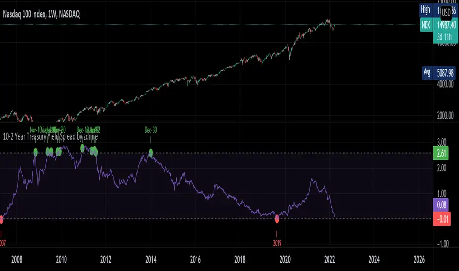
10-2 Year Treasury Yield Spread by zdmreLong-term bond yield reflects inflation. Short-term bond yields are tools used to predict Fed's interest rate policy. Spread between the two represents four cycles of an economy.
1. Growth
Short-term yield rises as interest rates rise. Spread narrows.
2. Slow growth
Central bank raises interest rates faster and short-term yield exceeds long-term yield. Spread turns negative.
3. Recession
High interest rates lead to more defaults. Inflation caps consumption. Central bank lowers interest rate to stimulate the economy and short-term yield falls. Spread widens.
4. Recovery
Central bank continues easing. Spread remains wide and yield curve remains steep.
0 = Recession Risk
2.6 = Recovery Plan
DYOR
6 Figures Scalping 2x MACD10-11-2019
This script plots a double MACD in a new indicator pane
The default settings:
Pink = STD MACD , settings 12-26-9
Green - Fast MACD, settings 5-15-1
The MACD settings can be changed in the indicators setting window

10/20/50/100/200 SMA'sMultiple MA's to get a good feel for momentum and interim supports and resistances


Moving Average x10 (SMA, EMA)10 configurable Simple and Exponential moving averages combined in one indicator
SMA RIBBON10 SMA's arranged in a ribbon. Color coded depending on price close. Free to use, open source. As seen in some charts.

10Y Bond Yield Spread (beta)10-Year Bond Yield Spread using Quandl data
See also:
- seekingalpha.com
- www.babypips.com
- www.forexfactory.com

10 Simple & 6 Exponential Moving Averages (w/ 18 day,week,month)* This is for the trader who wants tons of moving averages on their chart from one indicator
* Using the options, you should be able ot turn off some of them if the screen is too noisy for you
* You should also be able to change colors and thickness of the bars
* The thicker bars are for longer term averages
* This version is similar to my other script except it adds the 18 day, 18 week, and 18 Month SMa
* I added them after watching ira Epstein's YouTube videos
* Let me know if there are any bugs or things that need to be change

Advanced Trading System - Volume Profile + BB + RSI + FVG + FibAdvanced Multi-Indicator Trading System with Volume Profile, Bollinger Bands, RSI, FVG & Fibonacci
Overview
This comprehensive trading indicator combines five powerful technical analysis tools into one unified system, designed to identify high-probability trading opportunities with precision entry and exit signals. The indicator integrates Volume Profile analysis, Bollinger Bands, RSI momentum, Fair Value Gaps (FVG), and Fibonacci retracement levels to provide traders with a complete market analysis framework.
Key Features
1. Volume Profile & Point of Control (POC)
Automatically calculates the Point of Control - the price level with the highest trading volume
Identifies Value Area High (VAH) and Value Area Low (VAL)
Updates dynamically based on customizable lookback periods
Helps identify key support and resistance zones where institutional traders are active
2. Bollinger Bands Integration
Standard 20-period Bollinger Bands with customizable multiplier
Identifies overbought and oversold conditions
Measures market volatility through band width
Signals generated when price approaches extreme levels
3. RSI Momentum Analysis
14-period Relative Strength Index with visual background coloring
Overbought (70) and oversold (30) threshold alerts
Integrated into buy/sell signal logic for confirmation
Real-time momentum tracking in info dashboard
4. Fair Value Gap (FVG) Detection
Automatically identifies bullish and bearish fair value gaps
Visual representation with colored boxes
Highlights imbalance zones where price may return
Used for high-probability entry confirmation
5. Fibonacci Retracement Levels
Auto-calculated based on recent swing high/low
Key levels: 23.6%, 38.2%, 50%, 61.8%, 78.6%
Perfect for identifying profit-taking zones
Dynamic lines that update with market movement
6. Smart Signal Generation
The indicator generates BUY and SELL signals based on multi-condition confluence:
BUY Signal Requirements:
Price near lower Bollinger Band
RSI in oversold territory (< 30)
High volume confirmation (optional)
Bullish FVG or POC alignment
SELL Signal Requirements:
Price near upper Bollinger Band
RSI in overbought territory (> 70)
High volume confirmation (optional)
Bearish FVG or POC alignment
7. Automated Take Profit Levels
Three dynamic profit targets: 1%, 2%, and 3%
Automatically calculated from entry price
Visual markers on chart
Individual alerts for each level
8. Comprehensive Alert System
The indicator includes 10+ alert types:
Buy signal alerts
Sell signal alerts
Take profit level alerts (TP1, TP2, TP3)
Fibonacci level cross alerts
RSI overbought/oversold alerts
Bullish/Bearish FVG detection alerts
9. Real-Time Info Dashboard
Live display of all key metrics
Color-coded for quick visual analysis
Shows RSI, BB Width, Volume ratio, POC, Fib levels
Current signal status (BUY/SELL/WAIT)
How to Use
Setup
Add the indicator to your chart
Adjust parameters based on your trading style and timeframe
Set up alerts by clicking "Create Alert" and selecting desired conditions
Recommended Timeframes
Scalping: 5m - 15m
Day Trading: 15m - 1H
Swing Trading: 4H - Daily
Parameter Customization
Volume Profile Settings:
Length: 100 (adjust for more/less historical data)
Rows: 24 (granularity of volume distribution)
Bollinger Bands:
Length: 20 (standard period)
Multiplier: 2.0 (adjust for tighter/wider bands)
RSI Settings:
Length: 14 (standard momentum period)
Overbought: 70
Oversold: 30
Fibonacci:
Lookback: 50 (swing high/low detection period)
Signal Settings:
Volume Filter: Enable/disable volume confirmation
Volume MA Length: 20 (for volume comparison)
Trading Strategy Examples
Strategy 1: Trend Reversal
Wait for BUY signal at lower Bollinger Band
Confirm with bullish FVG or POC support
Enter position
Take partial profits at Fib 38.2% and 50%
Exit remaining position at TP3 or SELL signal
Strategy 2: Breakout Confirmation
Monitor price approaching POC level
Wait for volume spike
Enter on signal confirmation with FVG alignment
Use Fibonacci levels for scaling out
Strategy 3: Range Trading
Identify POC as range midpoint
Buy at lower BB with oversold RSI
Sell at upper BB with overbought RSI
Use FVG zones for additional confirmation
Best Practices
✅ Do:
Use multiple timeframe analysis
Combine with price action analysis
Set stop losses below/above recent swing points
Scale out at Fibonacci levels
Wait for volume confirmation on signals
❌ Don't:
Trade every signal blindly
Ignore overall market context
Use on extremely low timeframes without testing
Neglect risk management
Trade during low liquidity periods
Risk Management
Always use stop losses
Risk no more than 1-2% per trade
Consider market conditions and volatility
Scale position sizes based on signal strength
Use the volume filter for additional confirmation
Technical Specifications
Pine Script Version: 6
Overlay: Yes (displays on main chart)
Max Boxes: 500 (for FVG visualization)
Max Lines: 500 (for Fibonacci levels)
Alerts: 10+ customizable conditions
Performance Notes
This indicator works best in:
Trending markets with clear momentum
High-volume trading sessions
Assets with good liquidity
When multiple signals align
Less effective in:
Extremely choppy/sideways markets
Low-volume periods
During major news events (high volatility)
Updates & Support
This indicator is actively maintained and updated. Future enhancements may include:
Additional volume profile features
More sophisticated FVG tracking
Enhanced alert customization
Backtesting integration
Disclaimer
This indicator is for educational and informational purposes only. It does not constitute financial advice. Past performance does not guarantee future results. Always conduct your own research and consider consulting with a financial advisor before making trading decisions. Trading involves substantial risk of loss.

J&A Sessions & NewsProject J&A: Session Ranges is a precision-engineered tool designed for professional traders who operate based on Time & Price. Unlike standard session indicators that clutter the chart with background colors, this tool focuses on Dynamic Price Ranges to help you visualize the Highs, Lows, and liquidity pools of each session.
It is pre-configured for Frankfurt Time (Europe/Berlin) but is fully customizable for any global location.
Key Features
1. Dynamic Session Ranges (The Boxes) Instead of vertical stripes, this indicator draws Boxes that encapsulate the entire price action of a session.
Real-Time Tracking: The box automatically expands to capture the Highest High and Lowest Low of the current session.
Visual Clarity: Instantly see the trading range of Asia, London, and New York to identify breakouts or range-bound conditions.
2. The "Lunch Break" Logic (Unique Feature) Institutional volume often dies down during lunch hours. This indicator allows you to Split the Session to account for these breaks.
Enabled: The script draws two separate boxes (Morning Session vs. Afternoon Session), allowing you to see fresh ranges after the lunch accumulation.
Disabled: The script draws one continuous box for the full session.
3. Manual High-Impact News Scheduler Never get caught on the wrong side of a spike. Since TradingView scripts cannot access live calendars, this tool includes a Manual Scheduler for risk management.
Input: Simply input the time of high-impact events (e.g., CPI, NFP) from ForexFactory into the settings.
Visual: A dashed line appears on the chart at the exact news time.
Audio Alert: The system triggers an alarm 10 minutes before the event, giving you time to manage positions or exit trades.
Default Configuration (Frankfurt Time)
Asian Session: 01:00 - 10:00 (Lunch disabled)
London Session: 09:00 - 17:30 (Lunch: 12:00-13:00)
New York Session: 14:00 - 22:00 (Lunch: 18:00-19:00)
How to Use
Setup: Apply the indicator. The default timezone is Europe/Berlin. If you live elsewhere, simply change the "Your Timezone" setting to your local time (e.g., America/New_York), and the boxes will align automatically.
Daily Routine: Check the economic calendar in the morning. If there is a "Red Folder" event at 14:30, open the indicator settings and enter 14:30 into the News Scheduler.
Trade: Use the Session Highs and Lows as liquidity targets or breakout levels.
Settings & Customization
Timezone: Full support for major global trading hubs.
Colors: Customize the Box fill and Border colors for every session.
Labels: Rename sessions (e.g., "Tokyo" instead of "Asia") via the settings menu.

Dynamic Equity Allocation Model//@version=6
indicator('Dynamic Equity Allocation Model', shorttitle = 'DEAM', overlay = false, precision = 1, scale = scale.right, max_bars_back = 500)
// DYNAMIC EQUITY ALLOCATION MODEL
// Quantitative framework for dynamic portfolio allocation between stocks and cash.
// Analyzes five dimensions: market regime, risk metrics, valuation, sentiment,
// and macro conditions to generate allocation recommendations (0-100% equity).
//
// Uses real-time data from TradingView including fundamentals (P/E, ROE, ERP),
// volatility indicators (VIX), credit spreads, yield curves, and market structure.
// INPUT PARAMETERS
group1 = 'Model Configuration'
model_type = input.string('Adaptive', 'Allocation Model Type', options = , group = group1, tooltip = 'Conservative: Slower to increase equity, Aggressive: Faster allocation changes, Adaptive: Dynamic based on regime')
use_crisis_detection = input.bool(true, 'Enable Crisis Detection System', group = group1, tooltip = 'Automatic detection and response to crisis conditions')
use_regime_model = input.bool(true, 'Use Market Regime Detection', group = group1, tooltip = 'Identify Bull/Bear/Crisis regimes for dynamic allocation')
group2 = 'Portfolio Risk Management'
target_portfolio_volatility = input.float(12.0, 'Target Portfolio Volatility (%)', minval = 3, maxval = 20, step = 0.5, group = group2, tooltip = 'Target portfolio volatility (Cash reduces volatility: 50% Equity = ~10% vol, 100% Equity = ~20% vol)')
max_portfolio_drawdown = input.float(15.0, 'Maximum Portfolio Drawdown (%)', minval = 5, maxval = 35, step = 2.5, group = group2, tooltip = 'Maximum acceptable PORTFOLIO drawdown (not market drawdown - portfolio with cash has lower drawdown)')
enable_portfolio_risk_scaling = input.bool(true, 'Enable Portfolio Risk Scaling', group = group2, tooltip = 'Scale allocation based on actual portfolio risk characteristics (recommended)')
risk_lookback = input.int(252, 'Risk Calculation Period (Days)', minval = 60, maxval = 504, group = group2, tooltip = 'Period for calculating volatility and risk metrics')
group3 = 'Component Weights (Total = 100%)'
w_regime = input.float(35.0, 'Market Regime Weight (%)', minval = 0, maxval = 100, step = 5, group = group3)
w_risk = input.float(25.0, 'Risk Metrics Weight (%)', minval = 0, maxval = 100, step = 5, group = group3)
w_valuation = input.float(20.0, 'Valuation Weight (%)', minval = 0, maxval = 100, step = 5, group = group3)
w_sentiment = input.float(15.0, 'Sentiment Weight (%)', minval = 0, maxval = 100, step = 5, group = group3)
w_macro = input.float(5.0, 'Macro Weight (%)', minval = 0, maxval = 100, step = 5, group = group3)
group4 = 'Crisis Detection Thresholds'
crisis_vix_threshold = input.float(40, 'Crisis VIX Level', minval = 30, maxval = 80, group = group4, tooltip = 'VIX level indicating crisis conditions (COVID peaked at 82)')
crisis_drawdown_threshold = input.float(15, 'Crisis Drawdown Threshold (%)', minval = 10, maxval = 30, group = group4, tooltip = 'Market drawdown indicating crisis conditions')
crisis_credit_spread = input.float(500, 'Crisis Credit Spread (bps)', minval = 300, maxval = 1000, group = group4, tooltip = 'High yield spread indicating crisis conditions')
group5 = 'Display Settings'
show_components = input.bool(false, 'Show Component Breakdown', group = group5, tooltip = 'Display individual component analysis lines')
show_regime_background = input.bool(true, 'Show Dynamic Background', group = group5, tooltip = 'Color background based on allocation signals')
show_reference_lines = input.bool(false, 'Show Reference Lines', group = group5, tooltip = 'Display allocation percentage reference lines')
show_dashboard = input.bool(true, 'Show Analytics Dashboard', group = group5, tooltip = 'Display comprehensive analytics table')
show_confidence_bands = input.bool(false, 'Show Confidence Bands', group = group5, tooltip = 'Display uncertainty quantification bands')
smoothing_period = input.int(3, 'Smoothing Period', minval = 1, maxval = 10, group = group5, tooltip = 'Smoothing to reduce allocation noise')
background_intensity = input.int(95, 'Background Intensity (%)', minval = 90, maxval = 99, group = group5, tooltip = 'Higher values = more transparent background')
// Styling Options
color_scheme = input.string('EdgeTools', 'Color Theme', options = , group = 'Appearance', tooltip = 'Professional color themes')
use_dark_mode = input.bool(true, 'Optimize for Dark Theme', group = 'Appearance')
main_line_width = input.int(3, 'Main Line Width', minval = 1, maxval = 5, group = 'Appearance')
// DATA RETRIEVAL
// Market Data
sp500 = request.security('SPY', timeframe.period, close)
sp500_high = request.security('SPY', timeframe.period, high)
sp500_low = request.security('SPY', timeframe.period, low)
sp500_volume = request.security('SPY', timeframe.period, volume)
// Volatility Indicators
vix = request.security('VIX', timeframe.period, close)
vix9d = request.security('VIX9D', timeframe.period, close)
vxn = request.security('VXN', timeframe.period, close)
// Fixed Income and Credit
us2y = request.security('US02Y', timeframe.period, close)
us10y = request.security('US10Y', timeframe.period, close)
us3m = request.security('US03MY', timeframe.period, close)
hyg = request.security('HYG', timeframe.period, close)
lqd = request.security('LQD', timeframe.period, close)
tlt = request.security('TLT', timeframe.period, close)
// Safe Haven Assets
gold = request.security('GLD', timeframe.period, close)
usd = request.security('DXY', timeframe.period, close)
yen = request.security('JPYUSD', timeframe.period, close)
// Financial data with fallback values
get_financial_data(symbol, fin_id, period, fallback) =>
data = request.financial(symbol, fin_id, period, ignore_invalid_symbol = true)
na(data) ? fallback : data
// SPY fundamental metrics
spy_earnings_per_share = get_financial_data('AMEX:SPY', 'EARNINGS_PER_SHARE_BASIC', 'TTM', 20.0)
spy_operating_earnings_yield = get_financial_data('AMEX:SPY', 'OPERATING_EARNINGS_YIELD', 'FY', 4.5)
spy_dividend_yield = get_financial_data('AMEX:SPY', 'DIVIDENDS_YIELD', 'FY', 1.8)
spy_buyback_yield = get_financial_data('AMEX:SPY', 'BUYBACK_YIELD', 'FY', 2.0)
spy_net_margin = get_financial_data('AMEX:SPY', 'NET_MARGIN', 'TTM', 12.0)
spy_debt_to_equity = get_financial_data('AMEX:SPY', 'DEBT_TO_EQUITY', 'FY', 0.5)
spy_return_on_equity = get_financial_data('AMEX:SPY', 'RETURN_ON_EQUITY', 'FY', 15.0)
spy_free_cash_flow = get_financial_data('AMEX:SPY', 'FREE_CASH_FLOW', 'TTM', 100000000)
spy_ebitda = get_financial_data('AMEX:SPY', 'EBITDA', 'TTM', 200000000)
spy_pe_forward = get_financial_data('AMEX:SPY', 'PRICE_EARNINGS_FORWARD', 'FY', 18.0)
spy_total_debt = get_financial_data('AMEX:SPY', 'TOTAL_DEBT', 'FY', 500000000)
spy_total_equity = get_financial_data('AMEX:SPY', 'TOTAL_EQUITY', 'FY', 1000000000)
spy_enterprise_value = get_financial_data('AMEX:SPY', 'ENTERPRISE_VALUE', 'FY', 30000000000)
spy_revenue_growth = get_financial_data('AMEX:SPY', 'REVENUE_ONE_YEAR_GROWTH', 'TTM', 5.0)
// Market Breadth Indicators
nya = request.security('NYA', timeframe.period, close)
rut = request.security('IWM', timeframe.period, close)
// Sector Performance
xlk = request.security('XLK', timeframe.period, close)
xlu = request.security('XLU', timeframe.period, close)
xlf = request.security('XLF', timeframe.period, close)
// MARKET REGIME DETECTION
// Calculate Market Trend
sma_20 = ta.sma(sp500, 20)
sma_50 = ta.sma(sp500, 50)
sma_200 = ta.sma(sp500, 200)
ema_10 = ta.ema(sp500, 10)
// Market Structure Score
trend_strength = 0.0
trend_strength := trend_strength + (sp500 > sma_20 ? 1 : -1)
trend_strength := trend_strength + (sp500 > sma_50 ? 1 : -1)
trend_strength := trend_strength + (sp500 > sma_200 ? 2 : -2)
trend_strength := trend_strength + (sma_50 > sma_200 ? 2 : -2)
// Volatility Regime
returns = math.log(sp500 / sp500 )
realized_vol_20d = ta.stdev(returns, 20) * math.sqrt(252) * 100
realized_vol_60d = ta.stdev(returns, 60) * math.sqrt(252) * 100
ewma_vol = ta.ema(math.pow(returns, 2), 20)
realized_vol = math.sqrt(ewma_vol * 252) * 100
vol_premium = vix - realized_vol
// Drawdown Calculation
running_max = ta.highest(sp500, risk_lookback)
current_drawdown = (running_max - sp500) / running_max * 100
// Regime Score
regime_score = 0.0
// Trend Component (40%)
if trend_strength >= 4
regime_score := regime_score + 40
regime_score
else if trend_strength >= 2
regime_score := regime_score + 30
regime_score
else if trend_strength >= 0
regime_score := regime_score + 20
regime_score
else if trend_strength >= -2
regime_score := regime_score + 10
regime_score
else
regime_score := regime_score + 0
regime_score
// Volatility Component (30%)
if vix < 15
regime_score := regime_score + 30
regime_score
else if vix < 20
regime_score := regime_score + 25
regime_score
else if vix < 25
regime_score := regime_score + 15
regime_score
else if vix < 35
regime_score := regime_score + 5
regime_score
else
regime_score := regime_score + 0
regime_score
// Drawdown Component (30%)
if current_drawdown < 3
regime_score := regime_score + 30
regime_score
else if current_drawdown < 7
regime_score := regime_score + 20
regime_score
else if current_drawdown < 12
regime_score := regime_score + 10
regime_score
else if current_drawdown < 20
regime_score := regime_score + 5
regime_score
else
regime_score := regime_score + 0
regime_score
// Classify Regime
market_regime = regime_score >= 80 ? 'Strong Bull' : regime_score >= 60 ? 'Bull Market' : regime_score >= 40 ? 'Neutral' : regime_score >= 20 ? 'Correction' : regime_score >= 10 ? 'Bear Market' : 'Crisis'
// RISK-BASED ALLOCATION
// Calculate Market Risk
parkinson_hl = math.log(sp500_high / sp500_low)
parkinson_vol = parkinson_hl / (2 * math.sqrt(math.log(2))) * math.sqrt(252) * 100
garman_klass_vol = math.sqrt((0.5 * math.pow(math.log(sp500_high / sp500_low), 2) - (2 * math.log(2) - 1) * math.pow(math.log(sp500 / sp500 ), 2)) * 252) * 100
market_volatility_20d = math.max(ta.stdev(returns, 20) * math.sqrt(252) * 100, parkinson_vol)
market_volatility_60d = ta.stdev(returns, 60) * math.sqrt(252) * 100
market_drawdown = current_drawdown
// Initialize risk allocation
risk_allocation = 50.0
if enable_portfolio_risk_scaling
// Volatility-based allocation
vol_based_allocation = target_portfolio_volatility / math.max(market_volatility_20d, 5.0) * 100
vol_based_allocation := math.max(0, math.min(100, vol_based_allocation))
// Drawdown-based allocation
dd_based_allocation = 100.0
if market_drawdown > 1.0
dd_based_allocation := max_portfolio_drawdown / market_drawdown * 100
dd_based_allocation := math.max(0, math.min(100, dd_based_allocation))
dd_based_allocation
// Combine (conservative)
risk_allocation := math.min(vol_based_allocation, dd_based_allocation)
// Dynamic adjustment
current_equity_estimate = 50.0
estimated_portfolio_vol = current_equity_estimate / 100 * market_volatility_20d
estimated_portfolio_dd = current_equity_estimate / 100 * market_drawdown
vol_utilization = estimated_portfolio_vol / target_portfolio_volatility
dd_utilization = estimated_portfolio_dd / max_portfolio_drawdown
risk_utilization = math.max(vol_utilization, dd_utilization)
risk_adjustment_factor = 1.0
if risk_utilization > 1.0
risk_adjustment_factor := math.exp(-0.5 * (risk_utilization - 1.0))
risk_adjustment_factor := math.max(0.5, risk_adjustment_factor)
risk_adjustment_factor
else if risk_utilization < 0.9
risk_adjustment_factor := 1.0 + 0.2 * math.log(1.0 / risk_utilization)
risk_adjustment_factor := math.min(1.3, risk_adjustment_factor)
risk_adjustment_factor
risk_allocation := risk_allocation * risk_adjustment_factor
risk_allocation
else
vol_scalar = target_portfolio_volatility / math.max(market_volatility_20d, 10)
vol_scalar := math.min(1.5, math.max(0.2, vol_scalar))
drawdown_penalty = 0.0
if current_drawdown > max_portfolio_drawdown
drawdown_penalty := (current_drawdown - max_portfolio_drawdown) / max_portfolio_drawdown
drawdown_penalty := math.min(1.0, drawdown_penalty)
drawdown_penalty
risk_allocation := 100 * vol_scalar * (1 - drawdown_penalty)
risk_allocation
risk_allocation := math.max(0, math.min(100, risk_allocation))
// VALUATION ANALYSIS
// Valuation Metrics
actual_pe_ratio = spy_earnings_per_share > 0 ? sp500 / spy_earnings_per_share : spy_pe_forward
actual_earnings_yield = nz(spy_operating_earnings_yield, 0) > 0 ? spy_operating_earnings_yield : 100 / actual_pe_ratio
total_shareholder_yield = spy_dividend_yield + spy_buyback_yield
// Equity Risk Premium (multi-method calculation)
method1_erp = actual_earnings_yield - us10y
method2_erp = actual_earnings_yield + spy_buyback_yield - us10y
payout_ratio = spy_dividend_yield > 0 and actual_earnings_yield > 0 ? spy_dividend_yield / actual_earnings_yield : 0.4
sustainable_growth = spy_return_on_equity * (1 - payout_ratio) / 100
method3_erp = spy_dividend_yield + sustainable_growth * 100 - us10y
implied_growth = spy_revenue_growth * 0.7
method4_erp = total_shareholder_yield + implied_growth - us10y
equity_risk_premium = method1_erp * 0.35 + method2_erp * 0.30 + method3_erp * 0.20 + method4_erp * 0.15
ev_ebitda_ratio = spy_enterprise_value > 0 and spy_ebitda > 0 ? spy_enterprise_value / spy_ebitda : 15.0
debt_equity_health = spy_debt_to_equity < 1.0 ? 1.2 : spy_debt_to_equity < 2.0 ? 1.0 : 0.8
// Valuation Score
base_valuation_score = 50.0
if equity_risk_premium > 4
base_valuation_score := 95
base_valuation_score
else if equity_risk_premium > 3
base_valuation_score := 85
base_valuation_score
else if equity_risk_premium > 2
base_valuation_score := 70
base_valuation_score
else if equity_risk_premium > 1
base_valuation_score := 55
base_valuation_score
else if equity_risk_premium > 0
base_valuation_score := 40
base_valuation_score
else if equity_risk_premium > -1
base_valuation_score := 25
base_valuation_score
else
base_valuation_score := 10
base_valuation_score
growth_adjustment = spy_revenue_growth > 10 ? 10 : spy_revenue_growth > 5 ? 5 : 0
margin_adjustment = spy_net_margin > 15 ? 5 : spy_net_margin < 8 ? -5 : 0
roe_adjustment = spy_return_on_equity > 20 ? 5 : spy_return_on_equity < 10 ? -5 : 0
valuation_score = base_valuation_score + growth_adjustment + margin_adjustment + roe_adjustment
valuation_score := math.max(0, math.min(100, valuation_score * debt_equity_health))
// SENTIMENT ANALYSIS
// VIX Term Structure
vix_term_structure = vix9d > 0 ? vix / vix9d : 1
backwardation = vix_term_structure > 1.05
steep_backwardation = vix_term_structure > 1.15
// Safe Haven Flows
gold_momentum = ta.roc(gold, 20)
dollar_momentum = ta.roc(usd, 20)
yen_momentum = ta.roc(yen, 20)
treasury_momentum = ta.roc(tlt, 20)
safe_haven_flow = gold_momentum * 0.3 + treasury_momentum * 0.3 + dollar_momentum * 0.25 + yen_momentum * 0.15
// Advanced Sentiment Analysis
vix_percentile = ta.percentrank(vix, 252)
vix_zscore = (vix - ta.sma(vix, 252)) / ta.stdev(vix, 252)
vix_momentum = ta.roc(vix, 5)
vvix_proxy = ta.stdev(vix_momentum, 20) * math.sqrt(252)
risk_reversal_proxy = (vix - realized_vol) / realized_vol
// Sentiment Score
base_sentiment = 50.0
vix_adjustment = 0.0
if vix_zscore < -1.5
vix_adjustment := 40
vix_adjustment
else if vix_zscore < -0.5
vix_adjustment := 20
vix_adjustment
else if vix_zscore < 0.5
vix_adjustment := 0
vix_adjustment
else if vix_zscore < 1.5
vix_adjustment := -20
vix_adjustment
else
vix_adjustment := -40
vix_adjustment
term_structure_adjustment = backwardation ? -15 : steep_backwardation ? -30 : 5
vvix_adjustment = vvix_proxy > 2.0 ? -10 : vvix_proxy < 1.0 ? 10 : 0
sentiment_score = base_sentiment + vix_adjustment + term_structure_adjustment + vvix_adjustment
sentiment_score := math.max(0, math.min(100, sentiment_score))
// MACRO ANALYSIS
// Yield Curve
yield_spread_2_10 = us10y - us2y
yield_spread_3m_10 = us10y - us3m
// Credit Conditions
hyg_return = ta.roc(hyg, 20)
lqd_return = ta.roc(lqd, 20)
tlt_return = ta.roc(tlt, 20)
hyg_duration = 4.0
lqd_duration = 8.0
tlt_duration = 17.0
hyg_log_returns = math.log(hyg / hyg )
lqd_log_returns = math.log(lqd / lqd )
hyg_volatility = ta.stdev(hyg_log_returns, 20) * math.sqrt(252)
lqd_volatility = ta.stdev(lqd_log_returns, 20) * math.sqrt(252)
hyg_yield_proxy = -math.log(hyg / hyg ) * 100
lqd_yield_proxy = -math.log(lqd / lqd ) * 100
tlt_yield = us10y
hyg_spread = (hyg_yield_proxy - tlt_yield) * 100
lqd_spread = (lqd_yield_proxy - tlt_yield) * 100
hyg_distance = (hyg - ta.lowest(hyg, 252)) / (ta.highest(hyg, 252) - ta.lowest(hyg, 252))
lqd_distance = (lqd - ta.lowest(lqd, 252)) / (ta.highest(lqd, 252) - ta.lowest(lqd, 252))
default_risk_proxy = 2.0 - (hyg_distance + lqd_distance)
credit_spread = hyg_spread * 0.5 + (hyg_volatility - lqd_volatility) * 1000 * 0.3 + default_risk_proxy * 200 * 0.2
credit_spread := math.max(50, credit_spread)
credit_market_health = hyg_return > lqd_return ? 1 : -1
flight_to_quality = tlt_return > (hyg_return + lqd_return) / 2
// Macro Score
macro_score = 50.0
yield_curve_score = 0
if yield_spread_2_10 > 1.5 and yield_spread_3m_10 > 2
yield_curve_score := 40
yield_curve_score
else if yield_spread_2_10 > 0.5 and yield_spread_3m_10 > 1
yield_curve_score := 30
yield_curve_score
else if yield_spread_2_10 > 0 and yield_spread_3m_10 > 0
yield_curve_score := 20
yield_curve_score
else if yield_spread_2_10 < 0 or yield_spread_3m_10 < 0
yield_curve_score := 10
yield_curve_score
else
yield_curve_score := 5
yield_curve_score
credit_conditions_score = 0
if credit_spread < 200 and not flight_to_quality
credit_conditions_score := 30
credit_conditions_score
else if credit_spread < 400 and credit_market_health > 0
credit_conditions_score := 20
credit_conditions_score
else if credit_spread < 600
credit_conditions_score := 15
credit_conditions_score
else if credit_spread < 1000
credit_conditions_score := 10
credit_conditions_score
else
credit_conditions_score := 0
credit_conditions_score
financial_stability_score = 0
if spy_debt_to_equity < 0.5 and spy_return_on_equity > 15
financial_stability_score := 20
financial_stability_score
else if spy_debt_to_equity < 1.0 and spy_return_on_equity > 10
financial_stability_score := 15
financial_stability_score
else if spy_debt_to_equity < 1.5
financial_stability_score := 10
financial_stability_score
else
financial_stability_score := 5
financial_stability_score
macro_score := yield_curve_score + credit_conditions_score + financial_stability_score
macro_score := math.max(0, math.min(100, macro_score))
// CRISIS DETECTION
crisis_indicators = 0
if vix > crisis_vix_threshold
crisis_indicators := crisis_indicators + 1
crisis_indicators
if vix > 60
crisis_indicators := crisis_indicators + 2
crisis_indicators
if current_drawdown > crisis_drawdown_threshold
crisis_indicators := crisis_indicators + 1
crisis_indicators
if current_drawdown > 25
crisis_indicators := crisis_indicators + 1
crisis_indicators
if credit_spread > crisis_credit_spread
crisis_indicators := crisis_indicators + 1
crisis_indicators
sp500_roc_5 = ta.roc(sp500, 5)
tlt_roc_5 = ta.roc(tlt, 5)
if sp500_roc_5 < -10 and tlt_roc_5 < -5
crisis_indicators := crisis_indicators + 2
crisis_indicators
volume_spike = sp500_volume > ta.sma(sp500_volume, 20) * 2
sp500_roc_1 = ta.roc(sp500, 1)
if volume_spike and sp500_roc_1 < -3
crisis_indicators := crisis_indicators + 1
crisis_indicators
is_crisis = crisis_indicators >= 3
is_severe_crisis = crisis_indicators >= 5
// FINAL ALLOCATION CALCULATION
// Convert regime to base allocation
regime_allocation = market_regime == 'Strong Bull' ? 100 : market_regime == 'Bull Market' ? 80 : market_regime == 'Neutral' ? 60 : market_regime == 'Correction' ? 40 : market_regime == 'Bear Market' ? 20 : 0
// Normalize weights
total_weight = w_regime + w_risk + w_valuation + w_sentiment + w_macro
w_regime_norm = w_regime / total_weight
w_risk_norm = w_risk / total_weight
w_valuation_norm = w_valuation / total_weight
w_sentiment_norm = w_sentiment / total_weight
w_macro_norm = w_macro / total_weight
// Calculate Weighted Allocation
weighted_allocation = regime_allocation * w_regime_norm + risk_allocation * w_risk_norm + valuation_score * w_valuation_norm + sentiment_score * w_sentiment_norm + macro_score * w_macro_norm
// Apply Crisis Override
if use_crisis_detection
if is_severe_crisis
weighted_allocation := math.min(weighted_allocation, 10)
weighted_allocation
else if is_crisis
weighted_allocation := math.min(weighted_allocation, 25)
weighted_allocation
// Model Type Adjustment
model_adjustment = 0.0
if model_type == 'Conservative'
model_adjustment := -10
model_adjustment
else if model_type == 'Aggressive'
model_adjustment := 10
model_adjustment
else if model_type == 'Adaptive'
recent_return = (sp500 - sp500 ) / sp500 * 100
if recent_return > 5
model_adjustment := 5
model_adjustment
else if recent_return < -5
model_adjustment := -5
model_adjustment
// Apply adjustment and bounds
final_allocation = weighted_allocation + model_adjustment
final_allocation := math.max(0, math.min(100, final_allocation))
// Smooth allocation
smoothed_allocation = ta.sma(final_allocation, smoothing_period)
// Calculate portfolio risk metrics (only for internal alerts)
actual_portfolio_volatility = smoothed_allocation / 100 * market_volatility_20d
actual_portfolio_drawdown = smoothed_allocation / 100 * current_drawdown
// VISUALIZATION
// Color definitions
var color primary_color = #2196F3
var color bullish_color = #4CAF50
var color bearish_color = #FF5252
var color neutral_color = #808080
var color text_color = color.white
var color bg_color = #000000
var color table_bg_color = #1E1E1E
var color header_bg_color = #2D2D2D
switch color_scheme // Apply color scheme
'Gold' =>
primary_color := use_dark_mode ? #FFD700 : #DAA520
bullish_color := use_dark_mode ? #FFA500 : #FF8C00
bearish_color := use_dark_mode ? #FF5252 : #D32F2F
neutral_color := use_dark_mode ? #C0C0C0 : #808080
text_color := use_dark_mode ? color.white : color.black
bg_color := use_dark_mode ? #000000 : #FFFFFF
table_bg_color := use_dark_mode ? #1A1A00 : #FFFEF0
header_bg_color := use_dark_mode ? #2D2600 : #F5F5DC
header_bg_color
'EdgeTools' =>
primary_color := use_dark_mode ? #4682B4 : #1E90FF
bullish_color := use_dark_mode ? #4CAF50 : #388E3C
bearish_color := use_dark_mode ? #FF5252 : #D32F2F
neutral_color := use_dark_mode ? #708090 : #696969
text_color := use_dark_mode ? color.white : color.black
bg_color := use_dark_mode ? #000000 : #FFFFFF
table_bg_color := use_dark_mode ? #0F1419 : #F0F8FF
header_bg_color := use_dark_mode ? #1E2A3A : #E6F3FF
header_bg_color
'Behavioral' =>
primary_color := #808080
bullish_color := #00FF00
bearish_color := #8B0000
neutral_color := #FFBF00
text_color := use_dark_mode ? color.white : color.black
bg_color := use_dark_mode ? #000000 : #FFFFFF
table_bg_color := use_dark_mode ? #1A1A1A : #F8F8F8
header_bg_color := use_dark_mode ? #2D2D2D : #E8E8E8
header_bg_color
'Quant' =>
primary_color := #808080
bullish_color := #FFA500
bearish_color := #8B0000
neutral_color := #4682B4
text_color := use_dark_mode ? color.white : color.black
bg_color := use_dark_mode ? #000000 : #FFFFFF
table_bg_color := use_dark_mode ? #0D0D0D : #FAFAFA
header_bg_color := use_dark_mode ? #1A1A1A : #F0F0F0
header_bg_color
'Ocean' =>
primary_color := use_dark_mode ? #20B2AA : #008B8B
bullish_color := use_dark_mode ? #00CED1 : #4682B4
bearish_color := use_dark_mode ? #FF4500 : #B22222
neutral_color := use_dark_mode ? #87CEEB : #2F4F4F
text_color := use_dark_mode ? #F0F8FF : #191970
bg_color := use_dark_mode ? #001F3F : #F0F8FF
table_bg_color := use_dark_mode ? #001A2E : #E6F7FF
header_bg_color := use_dark_mode ? #002A47 : #CCF2FF
header_bg_color
'Fire' =>
primary_color := use_dark_mode ? #FF6347 : #DC143C
bullish_color := use_dark_mode ? #FFD700 : #FF8C00
bearish_color := use_dark_mode ? #8B0000 : #800000
neutral_color := use_dark_mode ? #FFA500 : #CD853F
text_color := use_dark_mode ? #FFFAF0 : #2F1B14
bg_color := use_dark_mode ? #2F1B14 : #FFFAF0
table_bg_color := use_dark_mode ? #261611 : #FFF8F0
header_bg_color := use_dark_mode ? #3D241A : #FFE4CC
header_bg_color
'Matrix' =>
primary_color := use_dark_mode ? #00FF41 : #006400
bullish_color := use_dark_mode ? #39FF14 : #228B22
bearish_color := use_dark_mode ? #FF073A : #8B0000
neutral_color := use_dark_mode ? #00FFFF : #008B8B
text_color := use_dark_mode ? #C0FF8C : #003300
bg_color := use_dark_mode ? #0D1B0D : #F0FFF0
table_bg_color := use_dark_mode ? #0A1A0A : #E8FFF0
header_bg_color := use_dark_mode ? #112B11 : #CCFFCC
header_bg_color
'Arctic' =>
primary_color := use_dark_mode ? #87CEFA : #4169E1
bullish_color := use_dark_mode ? #00BFFF : #0000CD
bearish_color := use_dark_mode ? #FF1493 : #8B008B
neutral_color := use_dark_mode ? #B0E0E6 : #483D8B
text_color := use_dark_mode ? #F8F8FF : #191970
bg_color := use_dark_mode ? #191970 : #F8F8FF
table_bg_color := use_dark_mode ? #141B47 : #F0F8FF
header_bg_color := use_dark_mode ? #1E2A5C : #E0F0FF
header_bg_color
// Transparency settings
bg_transparency = use_dark_mode ? 85 : 92
zone_transparency = use_dark_mode ? 90 : 95
band_transparency = use_dark_mode ? 70 : 85
table_transparency = use_dark_mode ? 80 : 15
// Allocation color
alloc_color = smoothed_allocation >= 80 ? bullish_color : smoothed_allocation >= 60 ? color.new(bullish_color, 30) : smoothed_allocation >= 40 ? primary_color : smoothed_allocation >= 20 ? color.new(bearish_color, 30) : bearish_color
// Dynamic background
var color dynamic_bg_color = na
if show_regime_background
if smoothed_allocation >= 70
dynamic_bg_color := color.new(bullish_color, background_intensity)
dynamic_bg_color
else if smoothed_allocation <= 30
dynamic_bg_color := color.new(bearish_color, background_intensity)
dynamic_bg_color
else if smoothed_allocation > 60 or smoothed_allocation < 40
dynamic_bg_color := color.new(primary_color, math.min(99, background_intensity + 2))
dynamic_bg_color
bgcolor(dynamic_bg_color, title = 'Allocation Signal Background')
// Plot main allocation line
plot(smoothed_allocation, 'Equity Allocation %', color = alloc_color, linewidth = math.max(1, main_line_width))
// Reference lines (static colors for hline)
hline_bullish_color = color_scheme == 'Gold' ? use_dark_mode ? #FFA500 : #FF8C00 : color_scheme == 'EdgeTools' ? use_dark_mode ? #4CAF50 : #388E3C : color_scheme == 'Behavioral' ? #00FF00 : color_scheme == 'Quant' ? #FFA500 : color_scheme == 'Ocean' ? use_dark_mode ? #00CED1 : #4682B4 : color_scheme == 'Fire' ? use_dark_mode ? #FFD700 : #FF8C00 : color_scheme == 'Matrix' ? use_dark_mode ? #39FF14 : #228B22 : color_scheme == 'Arctic' ? use_dark_mode ? #00BFFF : #0000CD : #4CAF50
hline_bearish_color = color_scheme == 'Gold' ? use_dark_mode ? #FF5252 : #D32F2F : color_scheme == 'EdgeTools' ? use_dark_mode ? #FF5252 : #D32F2F : color_scheme == 'Behavioral' ? #8B0000 : color_scheme == 'Quant' ? #8B0000 : color_scheme == 'Ocean' ? use_dark_mode ? #FF4500 : #B22222 : color_scheme == 'Fire' ? use_dark_mode ? #8B0000 : #800000 : color_scheme == 'Matrix' ? use_dark_mode ? #FF073A : #8B0000 : color_scheme == 'Arctic' ? use_dark_mode ? #FF1493 : #8B008B : #FF5252
hline_primary_color = color_scheme == 'Gold' ? use_dark_mode ? #FFD700 : #DAA520 : color_scheme == 'EdgeTools' ? use_dark_mode ? #4682B4 : #1E90FF : color_scheme == 'Behavioral' ? #808080 : color_scheme == 'Quant' ? #808080 : color_scheme == 'Ocean' ? use_dark_mode ? #20B2AA : #008B8B : color_scheme == 'Fire' ? use_dark_mode ? #FF6347 : #DC143C : color_scheme == 'Matrix' ? use_dark_mode ? #00FF41 : #006400 : color_scheme == 'Arctic' ? use_dark_mode ? #87CEFA : #4169E1 : #2196F3
hline(show_reference_lines ? 100 : na, '100% Equity', color = color.new(hline_bullish_color, 70), linestyle = hline.style_dotted, linewidth = 1)
hline(show_reference_lines ? 80 : na, '80% Equity', color = color.new(hline_bullish_color, 40), linestyle = hline.style_dashed, linewidth = 1)
hline(show_reference_lines ? 60 : na, '60% Equity', color = color.new(hline_bullish_color, 60), linestyle = hline.style_dotted, linewidth = 1)
hline(50, '50% Balanced', color = color.new(hline_primary_color, 50), linestyle = hline.style_solid, linewidth = 2)
hline(show_reference_lines ? 40 : na, '40% Equity', color = color.new(hline_bearish_color, 60), linestyle = hline.style_dotted, linewidth = 1)
hline(show_reference_lines ? 20 : na, '20% Equity', color = color.new(hline_bearish_color, 40), linestyle = hline.style_dashed, linewidth = 1)
hline(show_reference_lines ? 0 : na, '0% Equity', color = color.new(hline_bearish_color, 70), linestyle = hline.style_dotted, linewidth = 1)
// Component plots
plot(show_components ? regime_allocation : na, 'Regime', color = color.new(#4ECDC4, 70), linewidth = 1)
plot(show_components ? risk_allocation : na, 'Risk', color = color.new(#FF6B6B, 70), linewidth = 1)
plot(show_components ? valuation_score : na, 'Valuation', color = color.new(#45B7D1, 70), linewidth = 1)
plot(show_components ? sentiment_score : na, 'Sentiment', color = color.new(#FFD93D, 70), linewidth = 1)
plot(show_components ? macro_score : na, 'Macro', color = color.new(#6BCF7F, 70), linewidth = 1)
// Confidence bands
upper_band = plot(show_confidence_bands ? math.min(100, smoothed_allocation + ta.stdev(smoothed_allocation, 20)) : na, color = color.new(neutral_color, band_transparency), display = display.none, title = 'Upper Band')
lower_band = plot(show_confidence_bands ? math.max(0, smoothed_allocation - ta.stdev(smoothed_allocation, 20)) : na, color = color.new(neutral_color, band_transparency), display = display.none, title = 'Lower Band')
fill(upper_band, lower_band, color = show_confidence_bands ? color.new(neutral_color, zone_transparency) : na, title = 'Uncertainty')
// DASHBOARD
if show_dashboard and barstate.islast
var table dashboard = table.new(position.top_right, 2, 20, border_width = 1, bgcolor = color.new(table_bg_color, table_transparency))
table.clear(dashboard, 0, 0, 1, 19)
// Header
header_color = color.new(header_bg_color, 20)
dashboard_text_color = text_color
table.cell(dashboard, 0, 0, 'DEAM', text_color = dashboard_text_color, bgcolor = header_color, text_size = size.normal)
table.cell(dashboard, 1, 0, model_type, text_color = dashboard_text_color, bgcolor = header_color, text_size = size.normal)
// Core metrics
table.cell(dashboard, 0, 1, 'Equity Allocation', text_color = dashboard_text_color, text_size = size.small)
table.cell(dashboard, 1, 1, str.tostring(smoothed_allocation, '##.#') + '%', text_color = alloc_color, text_size = size.small)
table.cell(dashboard, 0, 2, 'Cash Allocation', text_color = dashboard_text_color, text_size = size.small)
cash_color = 100 - smoothed_allocation > 70 ? bearish_color : primary_color
table.cell(dashboard, 1, 2, str.tostring(100 - smoothed_allocation, '##.#') + '%', text_color = cash_color, text_size = size.small)
// Signal
signal_text = 'NEUTRAL'
signal_color = primary_color
if smoothed_allocation >= 70
signal_text := 'BULLISH'
signal_color := bullish_color
signal_color
else if smoothed_allocation <= 30
signal_text := 'BEARISH'
signal_color := bearish_color
signal_color
table.cell(dashboard, 0, 3, 'Signal', text_color = dashboard_text_color, text_size = size.small)
table.cell(dashboard, 1, 3, signal_text, text_color = signal_color, text_size = size.small)
// Market Regime
table.cell(dashboard, 0, 4, 'Regime', text_color = dashboard_text_color, text_size = size.small)
regime_color_display = market_regime == 'Strong Bull' or market_regime == 'Bull Market' ? bullish_color : market_regime == 'Neutral' ? primary_color : market_regime == 'Crisis' ? bearish_color : bearish_color
table.cell(dashboard, 1, 4, market_regime, text_color = regime_color_display, text_size = size.small)
// VIX
table.cell(dashboard, 0, 5, 'VIX Level', text_color = dashboard_text_color, text_size = size.small)
vix_color_display = vix < 20 ? bullish_color : vix < 30 ? primary_color : bearish_color
table.cell(dashboard, 1, 5, str.tostring(vix, '##.##'), text_color = vix_color_display, text_size = size.small)
// Market Drawdown
table.cell(dashboard, 0, 6, 'Market DD', text_color = dashboard_text_color, text_size = size.small)
market_dd_color = current_drawdown < 5 ? bullish_color : current_drawdown < 10 ? primary_color : bearish_color
table.cell(dashboard, 1, 6, '-' + str.tostring(current_drawdown, '##.#') + '%', text_color = market_dd_color, text_size = size.small)
// Crisis Detection
table.cell(dashboard, 0, 7, 'Crisis Detection', text_color = dashboard_text_color, text_size = size.small)
crisis_text = is_severe_crisis ? 'SEVERE' : is_crisis ? 'CRISIS' : 'Normal'
crisis_display_color = is_severe_crisis or is_crisis ? bearish_color : bullish_color
table.cell(dashboard, 1, 7, crisis_text, text_color = crisis_display_color, text_size = size.small)
// Real Data Section
financial_bg = color.new(primary_color, 85)
table.cell(dashboard, 0, 8, 'REAL DATA', text_color = dashboard_text_color, bgcolor = financial_bg, text_size = size.small)
table.cell(dashboard, 1, 8, 'Live Metrics', text_color = dashboard_text_color, bgcolor = financial_bg, text_size = size.small)
// P/E Ratio
table.cell(dashboard, 0, 9, 'P/E Ratio', text_color = dashboard_text_color, text_size = size.small)
pe_color = actual_pe_ratio < 18 ? bullish_color : actual_pe_ratio < 25 ? primary_color : bearish_color
table.cell(dashboard, 1, 9, str.tostring(actual_pe_ratio, '##.#'), text_color = pe_color, text_size = size.small)
// ERP
table.cell(dashboard, 0, 10, 'ERP', text_color = dashboard_text_color, text_size = size.small)
erp_color = equity_risk_premium > 2 ? bullish_color : equity_risk_premium > 0 ? primary_color : bearish_color
table.cell(dashboard, 1, 10, str.tostring(equity_risk_premium, '##.##') + '%', text_color = erp_color, text_size = size.small)
// ROE
table.cell(dashboard, 0, 11, 'ROE', text_color = dashboard_text_color, text_size = size.small)
roe_color = spy_return_on_equity > 20 ? bullish_color : spy_return_on_equity > 10 ? primary_color : bearish_color
table.cell(dashboard, 1, 11, str.tostring(spy_return_on_equity, '##.#') + '%', text_color = roe_color, text_size = size.small)
// D/E Ratio
table.cell(dashboard, 0, 12, 'D/E Ratio', text_color = dashboard_text_color, text_size = size.small)
de_color = spy_debt_to_equity < 0.5 ? bullish_color : spy_debt_to_equity < 1.0 ? primary_color : bearish_color
table.cell(dashboard, 1, 12, str.tostring(spy_debt_to_equity, '##.##'), text_color = de_color, text_size = size.small)
// Shareholder Yield
table.cell(dashboard, 0, 13, 'Dividend+Buyback', text_color = dashboard_text_color, text_size = size.small)
yield_color = total_shareholder_yield > 4 ? bullish_color : total_shareholder_yield > 2 ? primary_color : bearish_color
table.cell(dashboard, 1, 13, str.tostring(total_shareholder_yield, '##.#') + '%', text_color = yield_color, text_size = size.small)
// Component Scores
component_bg = color.new(neutral_color, 80)
table.cell(dashboard, 0, 14, 'Components', text_color = dashboard_text_color, bgcolor = component_bg, text_size = size.small)
table.cell(dashboard, 1, 14, 'Scores', text_color = dashboard_text_color, bgcolor = component_bg, text_size = size.small)
table.cell(dashboard, 0, 15, 'Regime', text_color = dashboard_text_color, text_size = size.small)
regime_score_color = regime_allocation > 60 ? bullish_color : regime_allocation < 40 ? bearish_color : primary_color
table.cell(dashboard, 1, 15, str.tostring(regime_allocation, '##'), text_color = regime_score_color, text_size = size.small)
table.cell(dashboard, 0, 16, 'Risk', text_color = dashboard_text_color, text_size = size.small)
risk_score_color = risk_allocation > 60 ? bullish_color : risk_allocation < 40 ? bearish_color : primary_color
table.cell(dashboard, 1, 16, str.tostring(risk_allocation, '##'), text_color = risk_score_color, text_size = size.small)
table.cell(dashboard, 0, 17, 'Valuation', text_color = dashboard_text_color, text_size = size.small)
val_score_color = valuation_score > 60 ? bullish_color : valuation_score < 40 ? bearish_color : primary_color
table.cell(dashboard, 1, 17, str.tostring(valuation_score, '##'), text_color = val_score_color, text_size = size.small)
table.cell(dashboard, 0, 18, 'Sentiment', text_color = dashboard_text_color, text_size = size.small)
sent_score_color = sentiment_score > 60 ? bullish_color : sentiment_score < 40 ? bearish_color : primary_color
table.cell(dashboard, 1, 18, str.tostring(sentiment_score, '##'), text_color = sent_score_color, text_size = size.small)
table.cell(dashboard, 0, 19, 'Macro', text_color = dashboard_text_color, text_size = size.small)
macro_score_color = macro_score > 60 ? bullish_color : macro_score < 40 ? bearish_color : primary_color
table.cell(dashboard, 1, 19, str.tostring(macro_score, '##'), text_color = macro_score_color, text_size = size.small)
// ALERTS
// Major allocation changes
alertcondition(smoothed_allocation >= 80 and smoothed_allocation < 80, 'High Equity Allocation', 'Equity allocation reached 80% - Bull market conditions')
alertcondition(smoothed_allocation <= 20 and smoothed_allocation > 20, 'Low Equity Allocation', 'Equity allocation dropped to 20% - Defensive positioning')
// Crisis alerts
alertcondition(is_crisis and not is_crisis , 'CRISIS DETECTED', 'Crisis conditions detected - Reducing equity allocation')
alertcondition(is_severe_crisis and not is_severe_crisis , 'SEVERE CRISIS', 'Severe crisis detected - Maximum defensive positioning')
// Regime changes
regime_changed = market_regime != market_regime
alertcondition(regime_changed, 'Regime Change', 'Market regime has changed')
// Risk management alerts
risk_breach = enable_portfolio_risk_scaling and (actual_portfolio_volatility > target_portfolio_volatility * 1.2 or actual_portfolio_drawdown > max_portfolio_drawdown * 1.2)
alertcondition(risk_breach, 'Risk Breach', 'Portfolio risk exceeds target parameters')
// USAGE
// The indicator displays a recommended equity allocation percentage (0-100%).
// Example: 75% allocation = 75% stocks, 25% cash/bonds.
//
// The model combines market regime analysis (trend, volatility, drawdowns),
// risk management (portfolio-level targeting), valuation metrics (P/E, ERP),
// sentiment indicators (VIX term structure), and macro factors (yield curve,
// credit spreads) into a single allocation signal.
//
// Crisis detection automatically reduces exposure when multiple warning signals
// converge. Alerts available for major allocation shifts and regime changes.
//
// Designed for SPY/S&P 500 portfolio allocation. Adjust component weights and
// risk parameters in settings to match your risk tolerance.
View in Pine

Hellenic EMA Matrix - PremiumHellenic EMA Matrix - Alpha Omega Premium
Complete User Guide
Table of Contents
Introduction
Indicator Philosophy
Mathematical Constants
EMA Types
Settings
Trading Signals
Visualization
Usage Strategies
FAQ
Introduction
Hellenic EMA Matrix is a premium indicator based on mathematical constants of nature: Phi (Phi - Golden Ratio), Pi (Pi), e (Euler's number). The indicator uses these universal constants to create dynamic EMAs that adapt to the natural rhythms of the market.
Key Features:
6 EMA types based on mathematical constants
Premium visualization with Neon Glow and Gradient Clouds
Automatic Fast/Mid/Slow EMA sorting
STRONG signals for powerful trends
Pulsing Ribbon Bar for instant trend assessment
Works on all timeframes (M1 - MN)
Indicator Philosophy
Why Mathematical Constants?
Traditional EMAs use arbitrary periods (9, 21, 50, 200). Hellenic Matrix goes further, using universal mathematical constants found in nature:
Phi (1.618) - Golden Ratio: galaxy spirals, seashells, human body proportions
Pi (3.14159) - Pi: circles, waves, cycles
e (2.71828) - Natural logarithm base: exponential growth, radioactive decay
Markets are also a natural system composed of millions of participants. Using mathematical constants allows tuning into the natural rhythms of market cycles.
Mathematical Constants
Phi (Phi) - Golden Ratio
Phi = 1.618033988749895
Properties:
Phi² = Phi + 1 = 2.618
Phi³ = 4.236
Phi⁴ = 6.854
Application: Ideal for trending movements and Fibonacci corrections
Pi (Pi) - Pi Number
Pi = 3.141592653589793
Properties:
2Pi = 6.283 (full circle)
3Pi = 9.425
4Pi = 12.566
Application: Excellent for cyclical markets and wave structures
e (Euler) - Euler's Number
e = 2.718281828459045
Properties:
e² = 7.389
e³ = 20.085
e⁴ = 54.598
Application: Suitable for exponential movements and volatile markets
EMA Types
1. Phi (Phi) - Golden Ratio EMA
Description: EMA based on the golden ratio
Period Formula:
Period = Phi^n × Base Multiplier
Parameters:
Phi Power Level (1-8): Power of Phi
Phi¹ = 1.618 → ~16 period (with Base=10)
Phi² = 2.618 → ~26 period
Phi³ = 4.236 → ~42 period (recommended)
Phi⁴ = 6.854 → ~69 period
Recommendations:
Phi² or Phi³ for day trading
Phi⁴ or Phi⁵ for swing trading
Works excellently as Fast EMA
2. Pi (Pi) - Circular EMA
Description: EMA based on Pi for cyclical movements
Period Formula:
Period = Pi × Multiple × Base Multiplier
Parameters:
Pi Multiple (1-10): Pi multiplier
1Pi = 3.14 → ~31 period (with Base=10)
2Pi = 6.28 → ~63 period (recommended)
3Pi = 9.42 → ~94 period
Recommendations:
2Pi ideal as Mid or Slow EMA
Excellently identifies cycles and waves
Use on volatile markets (crypto, forex)
3. e (Euler) - Natural EMA
Description: EMA based on natural logarithm
Period Formula:
Period = e^n × Base Multiplier
Parameters:
e Power Level (1-6): Power of e
e¹ = 2.718 → ~27 period (with Base=10)
e² = 7.389 → ~74 period (recommended)
e³ = 20.085 → ~201 period
Recommendations:
e² works excellently as Slow EMA
Ideal for stocks and indices
Filters noise well on lower timeframes
4. Delta (Delta) - Adaptive EMA
Description: Adaptive EMA that changes period based on volatility
Period Formula:
Period = Base Period × (1 + (Volatility - 1) × Factor)
Parameters:
Delta Base Period (5-200): Base period (default 20)
Delta Volatility Sensitivity (0.5-5.0): Volatility sensitivity (default 2.0)
How it works:
During low volatility → period decreases → EMA reacts faster
During high volatility → period increases → EMA smooths noise
Recommendations:
Works excellently on news and sharp movements
Use as Fast EMA for quick adaptation
Sensitivity 2.0-3.0 for crypto, 1.0-2.0 for stocks
5. Sigma (Sigma) - Composite EMA
Description: Composite EMA combining multiple active EMAs
Composition Methods:
Weighted Average (default):
Sigma = (Phi + Pi + e + Delta) / 4
Simple average of all active EMAs
Geometric Mean:
Sigma = fourth_root(Phi × Pi × e × Delta)
Geometric mean (more conservative)
Harmonic Mean:
Sigma = 4 / (1/Phi + 1/Pi + 1/e + 1/Delta)
Harmonic mean (more weight to smaller values)
Recommendations:
Enable for additional confirmation
Use as Mid EMA
Weighted Average - most universal method
6. Lambda (Lambda) - Wave EMA
Description: Wave EMA with sinusoidal period modulation
Period Formula:
Period = Base Period × (1 + Amplitude × sin(2Pi × bar / Frequency))
Parameters:
Lambda Base Period (10-200): Base period
Lambda Wave Amplitude (0.1-2.0): Wave amplitude
Lambda Wave Frequency (10-200): Wave frequency in bars
How it works:
Period pulsates sinusoidally
Creates wave effect following market cycles
Recommendations:
Experimental EMA for advanced users
Works well on cyclical markets
Frequency = 50 for day trading, 100+ for swing
Settings
Matrix Core Settings
Base Multiplier (1-100)
Multiplies all EMA periods
Base = 1: Very fast EMAs (Phi³ = 4, 2Pi = 6, e² = 7)
Base = 10: Standard (Phi³ = 42, 2Pi = 63, e² = 74)
Base = 20: Slow EMAs (Phi³ = 85, 2Pi = 126, e² = 148)
Recommendations by timeframe:
M1-M5: Base = 5-10
M15-H1: Base = 10-15 (recommended)
H4-D1: Base = 15-25
W1-MN: Base = 25-50
Matrix Source
Data source selection for EMA calculation:
close - closing price (standard)
open - opening price
high - high
low - low
hl2 - (high + low) / 2
hlc3 - (high + low + close) / 3
ohlc4 - (open + high + low + close) / 4
When to change:
hlc3 or ohlc4 for smoother signals
high for aggressive longs
low for aggressive shorts
Manual EMA Selection
Critically important setting! Determines which EMAs are used for signal generation.
Use Manual Fast/Slow/Mid Selection
Enabled (default): You select EMAs manually
Disabled: Automatic selection by periods
Fast EMA
Fast EMA - reacts first to price changes
Recommendations:
Phi Golden (recommended) - universal choice
Delta Adaptive - for volatile markets
Must be fastest (smallest period)
Slow EMA
Slow EMA - determines main trend
Recommendations:
Pi Circular (recommended) - excellent trend filter
e Natural - for smoother trend
Must be slowest (largest period)
Mid EMA
Mid EMA - additional signal filter
Recommendations:
e Natural (recommended) - excellent middle level
Pi Circular - alternative
None - for more frequent signals (only 2 EMAs)
IMPORTANT: The indicator automatically sorts selected EMAs by their actual periods:
Fast = EMA with smallest period
Mid = EMA with middle period
Slow = EMA with largest period
Therefore, you can select any combination - the indicator will arrange them correctly!
Premium Visualization
Neon Glow
Enable Neon Glow for EMAs - adds glowing effect around EMA lines
Glow Strength:
Light - subtle glow
Medium (recommended) - optimal balance
Strong - bright glow (may be too bright)
Effect: 2 glow layers around each EMA for 3D effect
Gradient Clouds
Enable Gradient Clouds - fills space between EMAs with gradient
Parameters:
Cloud Transparency (85-98): Cloud transparency
95-97 (recommended)
Higher = more transparent
Dynamic Cloud Intensity - automatically changes transparency based on EMA distance
Cloud Colors:
Phi-Pi Cloud:
Blue - when Pi above Phi (bullish)
Gold - when Phi above Pi (bearish)
Pi-e Cloud:
Green - when e above Pi (bullish)
Blue - when Pi above e (bearish)
2 layers for volumetric effect
Pulsing Ribbon Bar
Enable Pulsing Indicator Bar - pulsing strip at bottom/top of chart
Parameters:
Ribbon Position: Top / Bottom (recommended)
Pulse Speed: Slow / Medium (recommended) / Fast
Symbols and colors:
Green filled square - STRONG BULLISH
Pink filled square - STRONG BEARISH
Blue hollow square - Bullish (regular)
Red hollow square - Bearish (regular)
Purple rectangle - Neutral
Effect: Pulsation with sinusoid for living market feel
Signal Bar Highlights
Enable Signal Bar Highlights - highlights bars with signals
Parameters:
Highlight Transparency (88-96): Highlight transparency
Highlight Style:
Light Fill (recommended) - bar background fill
Thin Line - bar outline only
Highlights:
Golden Cross - green
Death Cross - pink
STRONG BUY - green
STRONG SELL - pink
Show Greek Labels
Shows Greek alphabet letters on last bar:
Phi - Phi EMA (gold)
Pi - Pi EMA (blue)
e - Euler EMA (green)
Delta - Delta EMA (purple)
Sigma - Sigma EMA (pink)
When to use: For education or presentations
Show Old Background
Old background style (not recommended):
Green background - STRONG BULLISH
Pink background - STRONG BEARISH
Blue background - Bullish
Red background - Bearish
Not recommended - use new Gradient Clouds and Pulsing Bar
Info Table
Show Info Table - table with indicator information
Parameters:
Position: Top Left / Top Right (recommended) / Bottom Left / Bottom Right
Size: Tiny / Small (recommended) / Normal / Large
Table contents:
EMA list - periods and current values of all active EMAs
Effects - active visual effects
TREND - current trend state:
STRONG UP - strong bullish
STRONG DOWN - strong bearish
Bullish - regular bullish
Bearish - regular bearish
Neutral - neutral
Momentum % - percentage deviation of price from Fast EMA
Setup - current Fast/Slow/Mid configuration
Trading Signals
Show Golden/Death Cross
Golden Cross - Fast EMA crosses Slow EMA from below (bullish signal) Death Cross - Fast EMA crosses Slow EMA from above (bearish signal)
Symbols:
Yellow dot "GC" below - Golden Cross
Dark red dot "DC" above - Death Cross
Show STRONG Signals
STRONG BUY and STRONG SELL - the most powerful indicator signals
Conditions for STRONG BULLISH:
EMA Alignment: Fast > Mid > Slow (all EMAs aligned)
Trend: Fast > Slow (clear uptrend)
Distance: EMAs separated by minimum 0.15%
Price Position: Price above Fast EMA
Fast Slope: Fast EMA rising
Slow Slope: Slow EMA rising
Mid Trending: Mid EMA also rising (if enabled)
Conditions for STRONG BEARISH:
Same but in reverse
Visual display:
Green label "STRONG BUY" below bar
Pink label "STRONG SELL" above bar
Difference from Golden/Death Cross:
Golden/Death Cross = crossing moment (1 bar)
STRONG signal = sustained trend (lasts several bars)
IMPORTANT: After fixes, STRONG signals now:
Work on all timeframes (M1 to MN)
Don't break on small retracements
Work with any Fast/Mid/Slow combination
Automatically adapt thanks to EMA sorting
Show Stop Loss/Take Profit
Automatic SL/TP level calculation on STRONG signal
Parameters:
Stop Loss (ATR) (0.5-5.0): ATR multiplier for stop loss
1.5 (recommended) - standard
1.0 - tight stop
2.0-3.0 - wide stop
Take Profit R:R (1.0-5.0): Risk/reward ratio
2.0 (recommended) - standard (risk 1.5 ATR, profit 3.0 ATR)
1.5 - conservative
3.0-5.0 - aggressive
Formulas:
LONG:
Stop Loss = Entry - (ATR × Stop Loss ATR)
Take Profit = Entry + (ATR × Stop Loss ATR × Take Profit R:R)
SHORT:
Stop Loss = Entry + (ATR × Stop Loss ATR)
Take Profit = Entry - (ATR × Stop Loss ATR × Take Profit R:R)
Visualization:
Red X - Stop Loss
Green X - Take Profit
Levels remain active while STRONG signal persists
Trading Signals
Signal Types
1. Golden Cross
Description: Fast EMA crosses Slow EMA from below
Signal: Beginning of bullish trend
How to trade:
ENTRY: On bar close with Golden Cross
STOP: Below local low or below Slow EMA
TARGET: Next resistance level or 2:1 R:R
Strengths:
Simple and clear
Works well on trending markets
Clear entry point
Weaknesses:
Lags (signal after movement starts)
Many false signals in ranging markets
May be late on fast moves
Optimal timeframes: H1, H4, D1
2. Death Cross
Description: Fast EMA crosses Slow EMA from above
Signal: Beginning of bearish trend
How to trade:
ENTRY: On bar close with Death Cross
STOP: Above local high or above Slow EMA
TARGET: Next support level or 2:1 R:R
Application: Mirror of Golden Cross
3. STRONG BUY
Description: All EMAs aligned + trend + all EMAs rising
Signal: Powerful bullish trend
How to trade:
ENTRY: On bar close with STRONG BUY or on pullback to Fast EMA
STOP: Below Fast EMA or automatic SL (if enabled)
TARGET: Automatic TP (if enabled) or by levels
TRAILING: Follow Fast EMA
Entry strategies:
Aggressive: Enter immediately on signal
Conservative: Wait for pullback to Fast EMA, then enter on bounce
Pyramiding: Add positions on pullbacks to Mid EMA
Position management:
Hold while STRONG signal active
Exit on STRONG SELL or Death Cross appearance
Move stop behind Fast EMA
Strengths:
Most reliable indicator signal
Doesn't break on pullbacks
Catches large moves
Works on all timeframes
Weaknesses:
Appears less frequently than other signals
Requires confirmation (multiple conditions)
Optimal timeframes: All (M5 - D1)
4. STRONG SELL
Description: All EMAs aligned down + downtrend + all EMAs falling
Signal: Powerful bearish trend
How to trade: Mirror of STRONG BUY
Visual Signals
Pulsing Ribbon Bar
Quick market assessment at a glance:
Symbol Color State
Filled square Green STRONG BULLISH
Filled square Pink STRONG BEARISH
Hollow square Blue Bullish
Hollow square Red Bearish
Rectangle Purple Neutral
Pulsation: Sinusoidal, creates living effect
Signal Bar Highlights
Bars with signals are highlighted:
Green highlight: STRONG BUY or Golden Cross
Pink highlight: STRONG SELL or Death Cross
Gradient Clouds
Colored space between EMAs shows trend strength:
Wide clouds - strong trend
Narrow clouds - weak trend or consolidation
Color change - trend change
Info Table
Quick reference in corner:
TREND: Current state (STRONG UP, Bullish, Neutral, Bearish, STRONG DOWN)
Momentum %: Movement strength
Effects: Active visual effects
Setup: Fast/Slow/Mid configuration
Usage Strategies
Strategy 1: "Golden Trailing"
Idea: Follow STRONG signals using Fast EMA as trailing stop
Settings:
Fast: Phi Golden (Phi³)
Mid: Pi Circular (2Pi)
Slow: e Natural (e²)
Base Multiplier: 10
Timeframe: H1, H4
Entry rules:
Wait for STRONG BUY
Enter on bar close or on pullback to Fast EMA
Stop below Fast EMA
Management:
Hold position while STRONG signal active
Move stop behind Fast EMA daily
Exit on STRONG SELL or Death Cross
Take Profit:
Partially close at +2R
Trail remainder until exit signal
For whom: Swing traders, trend followers
Pros:
Catches large moves
Simple rules
Emotionally comfortable
Cons:
Requires patience
Possible extended drawdowns on pullbacks
Strategy 2: "Scalping Bounces"
Idea: Scalp bounces from Fast EMA during STRONG trend
Settings:
Fast: Delta Adaptive (Base 15, Sensitivity 2.0)
Mid: Phi Golden (Phi²)
Slow: Pi Circular (2Pi)
Base Multiplier: 5
Timeframe: M5, M15
Entry rules:
STRONG signal must be active
Wait for price pullback to Fast EMA
Enter on bounce (candle closes above/below Fast EMA)
Stop behind local extreme (15-20 pips)
Take Profit:
+1.5R or to Mid EMA
Or to next level
For whom: Active day traders
Pros:
Many signals
Clear entry point
Quick profits
Cons:
Requires constant monitoring
Not all bounces work
Requires discipline for frequent trading
Strategy 3: "Triple Filter"
Idea: Enter only when all 3 EMAs and price perfectly aligned
Settings:
Fast: Phi Golden (Phi³)
Mid: e Natural (e²)
Slow: Pi Circular (3Pi)
Base Multiplier: 15
Timeframe: H4, D1
Entry rules (LONG):
STRONG BUY active
Price above all three EMAs
Fast > Mid > Slow (all aligned)
All EMAs rising (slope up)
Gradient Clouds wide and bright
Entry:
On bar close meeting all conditions
Or on next pullback to Fast EMA
Stop:
Below Mid EMA or -1.5 ATR
Take Profit:
First target: +3R
Second target: next major level
Trailing: Mid EMA
For whom: Conservative swing traders, investors
Pros:
Very reliable signals
Minimum false entries
Large profit potential
Cons:
Rare signals (2-5 per month)
Requires patience
Strategy 4: "Adaptive Scalper"
Idea: Use only Delta Adaptive EMA for quick volatility reaction
Settings:
Fast: Delta Adaptive (Base 10, Sensitivity 3.0)
Mid: None
Slow: Delta Adaptive (Base 30, Sensitivity 2.0)
Base Multiplier: 3
Timeframe: M1, M5
Feature: Two different Delta EMAs with different settings
Entry rules:
Golden Cross between two Delta EMAs
Both Delta EMAs must be rising/falling
Enter on next bar
Stop:
10-15 pips or below Slow Delta EMA
Take Profit:
+1R to +2R
Or Death Cross
For whom: Scalpers on cryptocurrencies and forex
Pros:
Instant volatility adaptation
Many signals on volatile markets
Quick results
Cons:
Much noise on calm markets
Requires fast execution
High commissions may eat profits
Strategy 5: "Cyclical Trader"
Idea: Use Pi and Lambda for trading cyclical markets
Settings:
Fast: Pi Circular (1Pi)
Mid: Lambda Wave (Base 30, Amplitude 0.5, Frequency 50)
Slow: Pi Circular (3Pi)
Base Multiplier: 10
Timeframe: H1, H4
Entry rules:
STRONG signal active
Lambda Wave EMA synchronized with trend
Enter on bounce from Lambda Wave
For whom: Traders of cyclical assets (some altcoins, commodities)
Pros:
Catches cyclical movements
Lambda Wave provides additional entry points
Cons:
More complex to configure
Not for all markets
Lambda Wave may give false signals
Strategy 6: "Multi-Timeframe Confirmation"
Idea: Use multiple timeframes for confirmation
Scheme:
Higher TF (D1): Determine trend direction (STRONG signal)
Middle TF (H4): Wait for STRONG signal in same direction
Lower TF (M15): Look for entry point (Golden Cross or bounce from Fast EMA)
Settings for all TFs:
Fast: Phi Golden (Phi³)
Mid: e Natural (e²)
Slow: Pi Circular (2Pi)
Base Multiplier: 10
Rules:
All 3 TFs must show one trend
Entry on lower TF
Stop by lower TF
Target by higher TF
For whom: Serious traders and investors
Pros:
Maximum reliability
Large profit targets
Minimum false signals
Cons:
Rare setups
Requires analysis of multiple charts
Experience needed
Practical Tips
DOs
Use STRONG signals as primary - they're most reliable
Let signals develop - don't exit on first pullback
Use trailing stop - follow Fast EMA
Combine with levels - S/R, Fibonacci, volumes
Test on demo before real
Adjust Base Multiplier for your timeframe
Enable visual effects - they help see the picture
Use Info Table - quick situation assessment
Watch Pulsing Bar - instant state indicator
Trust auto-sorting of Fast/Mid/Slow
DON'Ts
Don't trade against STRONG signal - trend is your friend
Don't ignore Mid EMA - it adds reliability
Don't use too small Base Multiplier on higher TFs
Don't enter on Golden Cross in range - check for trend
Don't change settings during open position
Don't forget risk management - 1-2% per trade
Don't trade all signals in row - choose best ones
Don't use indicator in isolation - combine with Price Action
Don't set too tight stops - let trade breathe
Don't over-optimize - simplicity = reliability
Optimal Settings by Asset
US Stocks (SPY, AAPL, TSLA)
Recommendation:
Fast: Phi Golden (Phi³)
Mid: e Natural (e²)
Slow: Pi Circular (2Pi)
Base: 10-15
Timeframe: H4, D1
Features:
Use on daily for swing
STRONG signals very reliable
Works well on trending stocks
Forex (EUR/USD, GBP/USD)
Recommendation:
Fast: Delta Adaptive (Base 15, Sens 2.0)
Mid: Phi Golden (Phi²)
Slow: Pi Circular (2Pi)
Base: 8-12
Timeframe: M15, H1, H4
Features:
Delta Adaptive works excellently on news
Many signals on M15-H1
Consider spreads
Cryptocurrencies (BTC, ETH, altcoins)
Recommendation:
Fast: Delta Adaptive (Base 10, Sens 3.0)
Mid: Pi Circular (2Pi)
Slow: e Natural (e²)
Base: 5-10
Timeframe: M5, M15, H1
Features:
High volatility - adaptation needed
STRONG signals can last days
Be careful with scalping on M1-M5
Commodities (Gold, Oil)
Recommendation:
Fast: Pi Circular (1Pi)
Mid: Phi Golden (Phi³)
Slow: Pi Circular (3Pi)
Base: 12-18
Timeframe: H4, D1
Features:
Pi works excellently on cyclical commodities
Gold responds especially well to Phi
Oil volatile - use wide stops
Indices (S&P500, Nasdaq, DAX)
Recommendation:
Fast: Phi Golden (Phi³)
Mid: e Natural (e²)
Slow: Pi Circular (2Pi)
Base: 15-20
Timeframe: H4, D1, W1
Features:
Very trending instruments
STRONG signals last weeks
Good for position trading
Alerts
The indicator supports 6 alert types:
1. Golden Cross
Message: "Hellenic Matrix: GOLDEN CROSS - Fast EMA crossed above Slow EMA - Bullish trend starting!"
When: Fast EMA crosses Slow EMA from below
2. Death Cross
Message: "Hellenic Matrix: DEATH CROSS - Fast EMA crossed below Slow EMA - Bearish trend starting!"
When: Fast EMA crosses Slow EMA from above
3. STRONG BULLISH
Message: "Hellenic Matrix: STRONG BULLISH SIGNAL - All EMAs aligned for powerful uptrend!"
When: All conditions for STRONG BUY met (first bar)
4. STRONG BEARISH
Message: "Hellenic Matrix: STRONG BEARISH SIGNAL - All EMAs aligned for powerful downtrend!"
When: All conditions for STRONG SELL met (first bar)
5. Bullish Ribbon
Message: "Hellenic Matrix: BULLISH RIBBON - EMAs aligned for uptrend"
When: EMAs aligned bullish + price above Fast EMA (less strict condition)
6. Bearish Ribbon
Message: "Hellenic Matrix: BEARISH RIBBON - EMAs aligned for downtrend"
When: EMAs aligned bearish + price below Fast EMA (less strict condition)
How to Set Up Alerts:
Open indicator on chart
Click on three dots next to indicator name
Select "Create Alert"
In "Condition" field select needed alert:
Golden Cross
Death Cross
STRONG BULLISH
STRONG BEARISH
Bullish Ribbon
Bearish Ribbon
Configure notification method:
Pop-up in browser
Email
SMS (in Premium accounts)
Push notifications in mobile app
Webhook (for automation)
Select frequency:
Once Per Bar Close (recommended) - once on bar close
Once Per Bar - during bar formation
Only Once - only first time
Click "Create"
Tip: Create separate alerts for different timeframes and instruments
FAQ
1. Why don't STRONG signals appear?
Possible reasons:
Incorrect Fast/Mid/Slow order
Solution: Indicator automatically sorts EMAs by periods, but ensure selected EMAs have different periods
Base Multiplier too large
Solution: Reduce Base to 5-10 on lower timeframes
Market in range
Solution: STRONG signals appear only in trends - this is normal
Too strict EMA settings
Solution: Try classic combination: Phi³ / Pi×2 / e² with Base=10
Mid EMA too close to Fast or Slow
Solution: Select Mid EMA with period between Fast and Slow
2. How often should STRONG signals appear?
Normal frequency:
M1-M5: 5-15 signals per day (very active markets)
M15-H1: 2-8 signals per day
H4: 3-10 signals per week
D1: 2-5 signals per month
W1: 2-6 signals per year
If too many signals - market very volatile or Base too small
If too few signals - market in range or Base too large
4. What are the best settings for beginners?
Universal "out of the box" settings:
Matrix Core:
Base Multiplier: 10
Source: close
Phi Golden: Enabled, Power = 3
Pi Circular: Enabled, Multiple = 2
e Natural: Enabled, Power = 2
Delta Adaptive: Enabled, Base = 20, Sensitivity = 2.0
Manual Selection:
Fast: Phi Golden
Mid: e Natural
Slow: Pi Circular
Visualization:
Gradient Clouds: ON
Neon Glow: ON (Medium)
Pulsing Bar: ON (Medium)
Signal Highlights: ON (Light Fill)
Table: ON (Top Right, Small)
Signals:
Golden/Death Cross: ON
STRONG Signals: ON
Stop Loss: OFF (while learning)
Timeframe for learning: H1 or H4
5. Can I use only one EMA?
No, minimum 2 EMAs (Fast and Slow) for signal generation.
Mid EMA is optional:
With Mid EMA = more reliable but rarer signals
Without Mid EMA = more signals but less strict filtering
Recommendation: Start with 3 EMAs (Fast/Mid/Slow), then experiment
6. Does the indicator work on cryptocurrencies?
Yes, works excellently! Especially good on:
Bitcoin (BTC)
Ethereum (ETH)
Major altcoins (SOL, BNB, XRP)
Recommended settings for crypto:
Fast: Delta Adaptive (Base 10-15, Sensitivity 2.5-3.0)
Mid: Pi Circular (2Pi)
Slow: e Natural (e²)
Base: 5-10
Timeframe: M15, H1, H4
Crypto market features:
High volatility → use Delta Adaptive
24/7 trading → set alerts
Sharp movements → wide stops
7. Can I trade only with this indicator?
Technically yes, but NOT recommended.
Best approach - combine with:
Price Action - support/resistance levels, candle patterns
Volume - movement strength confirmation
Fibonacci - retracement and extension levels
RSI/MACD - divergences and overbought/oversold
Fundamental analysis - news, company reports
Hellenic Matrix:
Excellently determines trend and its strength
Provides clear entry/exit points
Doesn't consider fundamentals
Doesn't see major levels
8. Why do Gradient Clouds change color?
Color depends on EMA order:
Phi-Pi Cloud:
Blue - Pi EMA above Phi EMA (bullish alignment)
Gold - Phi EMA above Pi EMA (bearish alignment)
Pi-e Cloud:
Green - e EMA above Pi EMA (bullish alignment)
Blue - Pi EMA above e EMA (bearish alignment)
Color change = EMA order change = possible trend change
9. What is Momentum % in the table?
Momentum % = percentage deviation of price from Fast EMA
Formula:
Momentum = ((Close - Fast EMA) / Fast EMA) × 100
Interpretation:
+0.5% to +2% - normal bullish momentum
+2% to +5% - strong bullish momentum
+5% and above - overheating (correction possible)
-0.5% to -2% - normal bearish momentum
-2% to -5% - strong bearish momentum
-5% and below - oversold (bounce possible)
Usage:
Monitor momentum during STRONG signals
Large momentum = don't enter (wait for pullback)
Small momentum = good entry point
10. How to configure for scalping?
Settings for scalping (M1-M5):
Base Multiplier: 3-5
Source: close or hlc3 (smoother)
Fast: Delta Adaptive (Base 8-12, Sensitivity 3.0)
Mid: None (for more signals)
Slow: Phi Golden (Phi²) or Pi Circular (1Pi)
Visualization:
- Gradient Clouds: ON (helps see strength)
- Neon Glow: OFF (doesn't clutter chart)
- Pulsing Bar: ON (quick assessment)
- Signal Highlights: ON
Signals:
- Golden/Death Cross: ON
- STRONG Signals: ON
- Stop Loss: ON (1.0-1.5 ATR, R:R 1.5-2.0)
Scalping rules:
Trade only STRONG signals
Enter on bounce from Fast EMA
Tight stops (10-20 pips)
Quick take profit (+1R to +2R)
Don't hold through news
11. How to configure for long-term investing?
Settings for investing (D1-W1):
Base Multiplier: 20-30
Source: close
Fast: Phi Golden (Phi³ or Phi⁴)
Mid: e Natural (e²)
Slow: Pi Circular (3Pi or 4Pi)
Visualization:
- Gradient Clouds: ON
- Neon Glow: ON (Medium)
- Everything else - to taste
Signals:
- Golden/Death Cross: ON
- STRONG Signals: ON
- Stop Loss: OFF (use percentage stop)
Investing rules:
Enter only on STRONG signals
Hold while STRONG active (weeks/months)
Stop below Slow EMA or -10%
Take profit: by company targets or +50-100%
Ignore short-term pullbacks
12. What if indicator slows down chart?
Indicator is optimized, but if it slows:
Disable unnecessary visual effects:
Neon Glow: OFF (saves 8 plots)
Gradient Clouds: ON but low quality
Lambda Wave EMA: OFF (if not using)
Reduce number of active EMAs:
Sigma Composite: OFF
Lambda Wave: OFF
Leave only Phi, Pi, e, Delta
Simplify settings:
Pulsing Bar: OFF
Greek Labels: OFF
Info Table: smaller size
13. Can I use on different timeframes simultaneously?
Yes! Multi-timeframe analysis is very powerful:
Classic scheme:
Higher TF (D1, W1) - determine global trend
Wait for STRONG signal
This is our trading direction
Middle TF (H4, H1) - look for confirmation
STRONG signal in same direction
Precise entry zone
Lower TF (M15, M5) - entry point
Golden Cross or bounce from Fast EMA
Precise stop loss
Example:
W1: STRONG BUY active (global uptrend)
H4: STRONG BUY appeared (confirmation)
M15: Wait for Golden Cross or bounce from Fast EMA → ENTRY
Advantages:
Maximum reliability
Clear timeframe hierarchy
Large targets
14. How does indicator work on news?
Delta Adaptive EMA adapts excellently to news:
Before news:
Low volatility → Delta EMA becomes fast → pulls to price
During news:
Sharp volatility spike → Delta EMA slows → filters noise
After news:
Volatility normalizes → Delta EMA returns to normal
Recommendations:
Don't trade at news release moment (spreads widen)
Wait for STRONG signal after news (2-5 bars)
Use Delta Adaptive as Fast EMA for quick reaction
Widen stops by 50-100% during important news
Advanced Techniques
Technique 1: "Divergences with EMA"
Idea: Look for discrepancies between price and Fast EMA
Bullish divergence:
Price makes lower low
Fast EMA makes higher low
= Possible reversal up
Bearish divergence:
Price makes higher high
Fast EMA makes lower high
= Possible reversal down
How to trade:
Find divergence
Wait for STRONG signal in divergence direction
Enter on confirmation
Technique 2: "EMA Tunnel"
Idea: Use space between Fast and Slow EMA as "tunnel"
Rules:
Wide tunnel - strong trend, hold position
Narrow tunnel - weak trend or consolidation, caution
Tunnel narrowing - trend weakening, prepare to exit
Tunnel widening - trend strengthening, can add
Visually: Gradient Clouds show this automatically!
Trading:
Enter on STRONG signal (tunnel starts widening)
Hold while tunnel wide
Exit when tunnel starts narrowing
Technique 3: "Wave Analysis with Lambda"
Idea: Lambda Wave EMA creates sinusoid matching market cycles
Setup:
Lambda Base Period: 30
Lambda Wave Amplitude: 0.5
Lambda Wave Frequency: 50 (adjusted to asset cycle)
How to find correct Frequency:
Look at historical cycles (distance between local highs)
Average distance = your Frequency
Example: if highs every 40-60 bars, set Frequency = 50
Trading:
Enter when Lambda Wave at bottom of sinusoid (growth potential)
Exit when Lambda Wave at top (fall potential)
Combine with STRONG signals
Technique 4: "Cluster Analysis"
Idea: When all EMAs gather in narrow cluster = powerful breakout soon
Cluster signs:
All EMAs (Phi, Pi, e, Delta) within 0.5-1% of each other
Gradient Clouds almost invisible
Price jumping around all EMAs
Trading:
Identify cluster (all EMAs close)
Determine breakout direction (where more volume, higher TFs direction)
Wait for breakout and STRONG signal
Enter on confirmation
Target = cluster size × 3-5
This is very powerful technique for big moves!
Technique 5: "Sigma as Dynamic Level"
Idea: Sigma Composite EMA = average of all EMAs = magnetic level
Usage:
Enable Sigma Composite (Weighted Average)
Sigma works as dynamic support/resistance
Price often returns to Sigma before trend continuation
Trading:
In trend: Enter on bounces from Sigma
In range: Fade moves from Sigma (trade return to Sigma)
On breakout: Sigma becomes support/resistance
Risk Management
Basic Rules
1. Position Size
Conservative: 1% of capital per trade
Moderate: 2% of capital per trade (recommended)
Aggressive: 3-5% (only for experienced)
Calculation formula:
Lot Size = (Capital × Risk%) / (Stop in pips × Pip value)
2. Risk/Reward Ratio
Minimum: 1:1.5
Standard: 1:2 (recommended)
Optimal: 1:3
Aggressive: 1:5+
3. Maximum Drawdown
Daily: -3% to -5%
Weekly: -7% to -10%
Monthly: -15% to -20%
Upon reaching limit → STOP trading until end of period
Position Management Strategies
1. Fixed Stop
Method:
Stop below/above Fast EMA or local extreme
DON'T move stop against position
Can move to breakeven
For whom: Beginners, conservative traders
2. Trailing by Fast EMA
Method:
Each day (or bar) move stop to Fast EMA level
Position closes when price breaks Fast EMA
Advantages:
Stay in trend as long as possible
Automatically exit on reversal
For whom: Trend followers, swing traders
3. Partial Exit
Method:
50% of position close at +2R
50% hold with trailing by Mid EMA or Slow EMA
Advantages:
Lock profit
Leave position for big move
Psychologically comfortable
For whom: Universal method (recommended)
4. Pyramiding
Method:
First entry on STRONG signal (50% of planned position)
Add 25% on pullback to Fast EMA
Add another 25% on pullback to Mid EMA
Overall stop below Slow EMA
Advantages:
Average entry price
Reduce risk
Increase profit in strong trends
Caution:
Works only in trends
In range leads to losses
For whom: Experienced traders
Trading Psychology
Correct Mindset
1. Indicator is a tool, not holy grail
Indicator shows probability, not guarantee
There will be losing trades - this is normal
Important is series statistics, not one trade
2. Trust the system
If STRONG signal appeared - enter
Don't search for "perfect" moment
Follow trading plan
3. Patience
STRONG signals don't appear every day
Better miss signal than enter against trend
Quality over quantity
4. Discipline
Always set stop loss
Don't move stop against position
Don't increase risk after losses
Beginner Mistakes
1. "I know better than indicator"
Indicator says STRONG BUY, but you think "too high, will wait for pullback"
Result: miss profitable move
Solution: Trust signals or don't use indicator
2. "Will reverse now for sure"
Trading against STRONG trend
Result: stops, stops, stops
Solution: Trend is your friend, trade with trend
3. "Will hold a bit more"
Don't exit when STRONG signal disappears
Greed eats profit
Solution: If signal gone - exit!
4. "I'll recover"
After losses double risk
Result: huge losses
Solution: Fixed % risk ALWAYS
5. "I don't like this signal"
Skip signals because of "feeling"
Result: inconsistency, no statistics
Solution: Trade ALL signals or clearly define filters
Trading Journal
What to Record
For each trade:
1. Entry/exit date and time
2. Instrument and timeframe
3. Signal type
Golden Cross
STRONG BUY
STRONG SELL
Death Cross
4. Indicator settings
Fast/Mid/Slow EMA
Base Multiplier
Other parameters
5. Chart screenshot
Entry moment
Exit moment
6. Trade parameters
Position size
Stop loss
Take Profit
R:R
7. Result
Profit/Loss in $
Profit/Loss in %
Profit/Loss in R
8. Notes
What was right
What was wrong
Emotions during trade
Lessons
Journal Analysis
Analyze weekly:
1. Win Rate
Win Rate = (Profitable trades / All trades) × 100%
Good: 50-60%
Excellent: 60-70%
Exceptional: 70%+
2. Average R
Average R = Sum of all R / Number of trades
Good: +0.5R
Excellent: +1.0R
Exceptional: +1.5R+
3. Profit Factor
Profit Factor = Total profit / Total losses
Good: 1.5+
Excellent: 2.0+
Exceptional: 3.0+
4. Maximum Drawdown
Track consecutive losses
If more than 5 in row - stop, check system
5. Best/Worst Trades
What was common in best trades? (do more)
What was common in worst trades? (avoid)
Pre-Trade Checklist
Technical Analysis
STRONG signal active (BUY or SELL)
All EMAs properly aligned (Fast > Mid > Slow or reverse)
Price on correct side of Fast EMA
Gradient Clouds confirm trend
Pulsing Bar shows STRONG state
Momentum % in normal range (not overheated)
No close strong levels against direction
Higher timeframe doesn't contradict
Risk Management
Position size calculated (1-2% risk)
Stop loss set
Take profit calculated (minimum 1:2)
R:R satisfactory
Daily/weekly risk limit not exceeded
No other open correlated positions
Fundamental Analysis
No important news in coming hours
Market session appropriate (liquidity)
No contradicting fundamentals
Understand why asset is moving
Psychology
Calm and thinking clearly
No emotions from previous trades
Ready to accept loss at stop
Following trading plan
Not revenging market for past losses
If at least one point is NO - think twice before entering!
Learning Roadmap
Week 1: Familiarization
Goals:
Install and configure indicator
Study all EMA types
Understand visualization
Tasks:
Add indicator to chart
Test all Fast/Mid/Slow settings
Play with Base Multiplier on different timeframes
Observe Gradient Clouds and Pulsing Bar
Study Info Table
Result: Comfort with indicator interface
Week 2: Signals
Goals:
Learn to recognize all signal types
Understand difference between Golden Cross and STRONG
Tasks:
Find 10 Golden Cross examples in history
Find 10 STRONG BUY examples in history
Compare their results (which worked better)
Set up alerts
Get 5 real alerts
Result: Understanding signals
Week 3: Demo Trading
Goals:
Start trading signals on demo account
Gather statistics
Tasks:
Open demo account
Trade ONLY STRONG signals
Keep journal (minimum 20 trades)
Don't change indicator settings
Strictly follow stop losses
Result: 20+ documented trades
Week 4: Analysis
Goals:
Analyze demo trading results
Optimize approach
Tasks:
Calculate win rate and average R
Find patterns in profitable trades
Find patterns in losing trades
Adjust approach (not indicator!)
Write trading plan
Result: Trading plan on 1 page
Month 2: Improvement
Goals:
Deepen understanding
Add additional techniques
Tasks:
Study multi-timeframe analysis
Test combinations with Price Action
Try advanced techniques (divergences, tunnels)
Continue demo trading (minimum 50 trades)
Achieve stable profitability on demo
Result: Win rate 55%+ and Profit Factor 1.5+
Month 3: Real Trading
Goals:
Transition to real account
Maintain discipline
Tasks:
Open small real account
Trade minimum lots
Strictly follow trading plan
DON'T increase risk
Focus on process, not profit
Result: Psychological comfort on real
Month 4+: Scaling
Goals:
Increase account
Become consistently profitable
Tasks:
With 60%+ win rate can increase risk to 2%
Upon doubling account can add capital
Continue keeping journal
Periodically review and improve strategy
Share experience with community
Result: Stable profitability month after month
Additional Resources
Recommended Reading
Technical Analysis:
"Technical Analysis of Financial Markets" - John Murphy
"Trading in the Zone" - Mark Douglas (psychology)
"Market Wizards" - Jack Schwager (trader interviews)
EMA and Moving Averages:
"Moving Averages 101" - Steve Burns
Articles on Investopedia about EMA
Risk Management:
"The Mathematics of Money Management" - Ralph Vince
"Trade Your Way to Financial Freedom" - Van K. Tharp
Trading Journals:
Edgewonk (paid, very powerful)
Tradervue (free version + premium)
Excel/Google Sheets (free)
Screeners:
TradingView Stock Screener
Finviz (stocks)
CoinMarketCap (crypto)
Conclusion
Hellenic EMA Matrix is a powerful tool based on universal mathematical constants of nature. The indicator combines:
Mathematical elegance - Phi, Pi, e instead of arbitrary numbers
Premium visualization - Neon Glow, Gradient Clouds, Pulsing Bar
Reliable signals - STRONG BUY/SELL work on all timeframes
Flexibility - 6 EMA types, adaptation to any trading style
Automation - auto-sorting EMAs, SL/TP calculation, alerts
Key Success Principles:
Simplicity - start with basic settings (Phi/Pi/e, Base=10)
Discipline - follow STRONG signals strictly
Patience - wait for quality setups
Risk Management - 1-2% per trade, ALWAYS
Journal - document every trade
Learning - constantly improve skills
Remember:
Indicator shows probability, not guarantee
Important is series statistics, not one trade
Psychology more important than technique
Quality more important than quantity
Process more important than result
Acknowledgments
Thank you for using Hellenic EMA Matrix - Alpha Omega Premium!
The indicator was created with love for mathematics, markets, and beautiful visualization.
Wishing you profitable trading!
Guide Version: 1.0
Date: 2025
Compatibility: Pine Script v6, TradingView
"In the simplicity of mathematical constants lies the complexity of market movements"

Markov Chain [3D] | FractalystWhat exactly is a Markov Chain?
This indicator uses a Markov Chain model to analyze, quantify, and visualize the transitions between market regimes (Bull, Bear, Neutral) on your chart. It dynamically detects these regimes in real-time, calculates transition probabilities, and displays them as animated 3D spheres and arrows, giving traders intuitive insight into current and future market conditions.
How does a Markov Chain work, and how should I read this spheres-and-arrows diagram?
Think of three weather modes: Sunny, Rainy, Cloudy.
Each sphere is one mode. The loop on a sphere means “stay the same next step” (e.g., Sunny again tomorrow).
The arrows leaving a sphere show where things usually go next if they change (e.g., Sunny moving to Cloudy).
Some paths matter more than others. A more prominent loop means the current mode tends to persist. A more prominent outgoing arrow means a change to that destination is the usual next step.
Direction isn’t symmetric: moving Sunny→Cloudy can behave differently than Cloudy→Sunny.
Now relabel the spheres to markets: Bull, Bear, Neutral.
Spheres: market regimes (uptrend, downtrend, range).
Self‑loop: tendency for the current regime to continue on the next bar.
Arrows: the most common next regime if a switch happens.
How to read: Start at the sphere that matches current bar state. If the loop stands out, expect continuation. If one outgoing path stands out, that switch is the typical next step. Opposite directions can differ (Bear→Neutral doesn’t have to match Neutral→Bear).
What states and transitions are shown?
The three market states visualized are:
Bullish (Bull): Upward or strong-market regime.
Bearish (Bear): Downward or weak-market regime.
Neutral: Sideways or range-bound regime.
Bidirectional animated arrows and probability labels show how likely the market is to move from one regime to another (e.g., Bull → Bear or Neutral → Bull).
How does the regime detection system work?
You can use either built-in price returns (based on adaptive Z-score normalization) or supply three custom indicators (such as volume, oscillators, etc.).
Values are statistically normalized (Z-scored) over a configurable lookback period.
The normalized outputs are classified into Bull, Bear, or Neutral zones.
If using three indicators, their regime signals are averaged and smoothed for robustness.
How are transition probabilities calculated?
On every confirmed bar, the algorithm tracks the sequence of detected market states, then builds a rolling window of transitions.
The code maintains a transition count matrix for all regime pairs (e.g., Bull → Bear).
Transition probabilities are extracted for each possible state change using Laplace smoothing for numerical stability, and frequently updated in real-time.
What is unique about the visualization?
3D animated spheres represent each regime and change visually when active.
Animated, bidirectional arrows reveal transition probabilities and allow you to see both dominant and less likely regime flows.
Particles (moving dots) animate along the arrows, enhancing the perception of regime flow direction and speed.
All elements dynamically update with each new price bar, providing a live market map in an intuitive, engaging format.
Can I use custom indicators for regime classification?
Yes! Enable the "Custom Indicators" switch and select any three chart series as inputs. These will be normalized and combined (each with equal weight), broadening the regime classification beyond just price-based movement.
What does the “Lookback Period” control?
Lookback Period (default: 100) sets how much historical data builds the probability matrix. Shorter periods adapt faster to regime changes but may be noisier. Longer periods are more stable but slower to adapt.
How is this different from a Hidden Markov Model (HMM)?
It sets the window for both regime detection and probability calculations. Lower values make the system more reactive, but potentially noisier. Higher values smooth estimates and make the system more robust.
How is this Markov Chain different from a Hidden Markov Model (HMM)?
Markov Chain (as here): All market regimes (Bull, Bear, Neutral) are directly observable on the chart. The transition matrix is built from actual detected regimes, keeping the model simple and interpretable.
Hidden Markov Model: The actual regimes are unobservable ("hidden") and must be inferred from market output or indicator "emissions" using statistical learning algorithms. HMMs are more complex, can capture more subtle structure, but are harder to visualize and require additional machine learning steps for training.
A standard Markov Chain models transitions between observable states using a simple transition matrix, while a Hidden Markov Model assumes the true states are hidden (latent) and must be inferred from observable “emissions” like price or volume data. In practical terms, a Markov Chain is transparent and easier to implement and interpret; an HMM is more expressive but requires statistical inference to estimate hidden states from data.
Markov Chain: states are observable; you directly count or estimate transition probabilities between visible states. This makes it simpler, faster, and easier to validate and tune.
HMM: states are hidden; you only observe emissions generated by those latent states. Learning involves machine learning/statistical algorithms (commonly Baum–Welch/EM for training and Viterbi for decoding) to infer both the transition dynamics and the most likely hidden state sequence from data.
How does the indicator avoid “repainting” or look-ahead bias?
All regime changes and matrix updates happen only on confirmed (closed) bars, so no future data is leaked, ensuring reliable real-time operation.
Are there practical tuning tips?
Tune the Lookback Period for your asset/timeframe: shorter for fast markets, longer for stability.
Use custom indicators if your asset has unique regime drivers.
Watch for rapid changes in transition probabilities as early warning of a possible regime shift.
Who is this indicator for?
Quants and quantitative researchers exploring probabilistic market modeling, especially those interested in regime-switching dynamics and Markov models.
Programmers and system developers who need a probabilistic regime filter for systematic and algorithmic backtesting:
The Markov Chain indicator is ideally suited for programmatic integration via its bias output (1 = Bull, 0 = Neutral, -1 = Bear).
Although the visualization is engaging, the core output is designed for automated, rules-based workflows—not for discretionary/manual trading decisions.
Developers can connect the indicator’s output directly to their Pine Script logic (using input.source()), allowing rapid and robust backtesting of regime-based strategies.
It acts as a plug-and-play regime filter: simply plug the bias output into your entry/exit logic, and you have a scientifically robust, probabilistically-derived signal for filtering, timing, position sizing, or risk regimes.
The MC's output is intentionally "trinary" (1/0/-1), focusing on clear regime states for unambiguous decision-making in code. If you require nuanced, multi-probability or soft-label state vectors, consider expanding the indicator or stacking it with a probability-weighted logic layer in your scripting.
Because it avoids subjectivity, this approach is optimal for systematic quants, algo developers building backtested, repeatable strategies based on probabilistic regime analysis.
What's the mathematical foundation behind this?
The mathematical foundation behind this Markov Chain indicator—and probabilistic regime detection in finance—draws from two principal models: the (standard) Markov Chain and the Hidden Markov Model (HMM).
How to use this indicator programmatically?
The Markov Chain indicator automatically exports a bias value (+1 for Bullish, -1 for Bearish, 0 for Neutral) as a plot visible in the Data Window. This allows you to integrate its regime signal into your own scripts and strategies for backtesting, automation, or live trading.
Step-by-Step Integration with Pine Script (input.source)
Add the Markov Chain indicator to your chart.
This must be done first, since your custom script will "pull" the bias signal from the indicator's plot.
In your strategy, create an input using input.source()
Example:
//@version=5
strategy("MC Bias Strategy Example")
mcBias = input.source(close, "MC Bias Source")
After saving, go to your script’s settings. For the “MC Bias Source” input, select the plot/output of the Markov Chain indicator (typically its bias plot).
Use the bias in your trading logic
Example (long only on Bull, flat otherwise):
if mcBias == 1
strategy.entry("Long", strategy.long)
else
strategy.close("Long")
For more advanced workflows, combine mcBias with additional filters or trailing stops.
How does this work behind-the-scenes?
TradingView’s input.source() lets you use any plot from another indicator as a real-time, “live” data feed in your own script (source).
The selected bias signal is available to your Pine code as a variable, enabling logical decisions based on regime (trend-following, mean-reversion, etc.).
This enables powerful strategy modularity : decouple regime detection from entry/exit logic, allowing fast experimentation without rewriting core signal code.
Integrating 45+ Indicators with Your Markov Chain — How & Why
The Enhanced Custom Indicators Export script exports a massive suite of over 45 technical indicators—ranging from classic momentum (RSI, MACD, Stochastic, etc.) to trend, volume, volatility, and oscillator tools—all pre-calculated, centered/scaled, and available as plots.
// Enhanced Custom Indicators Export - 45 Technical Indicators
// Comprehensive technical analysis suite for advanced market regime detection
//@version=6
indicator('Enhanced Custom Indicators Export | Fractalyst', shorttitle='Enhanced CI Export', overlay=false, scale=scale.right, max_labels_count=500, max_lines_count=500)
// |----- Input Parameters -----| //
momentum_group = "Momentum Indicators"
trend_group = "Trend Indicators"
volume_group = "Volume Indicators"
volatility_group = "Volatility Indicators"
oscillator_group = "Oscillator Indicators"
display_group = "Display Settings"
// Common lengths
length_14 = input.int(14, "Standard Length (14)", minval=1, maxval=100, group=momentum_group)
length_20 = input.int(20, "Medium Length (20)", minval=1, maxval=200, group=trend_group)
length_50 = input.int(50, "Long Length (50)", minval=1, maxval=200, group=trend_group)
// Display options
show_table = input.bool(true, "Show Values Table", group=display_group)
table_size = input.string("Small", "Table Size", options= , group=display_group)
// |----- MOMENTUM INDICATORS (15 indicators) -----| //
// 1. RSI (Relative Strength Index)
rsi_14 = ta.rsi(close, length_14)
rsi_centered = rsi_14 - 50
// 2. Stochastic Oscillator
stoch_k = ta.stoch(close, high, low, length_14)
stoch_d = ta.sma(stoch_k, 3)
stoch_centered = stoch_k - 50
// 3. Williams %R
williams_r = ta.stoch(close, high, low, length_14) - 100
// 4. MACD (Moving Average Convergence Divergence)
= ta.macd(close, 12, 26, 9)
// 5. Momentum (Rate of Change)
momentum = ta.mom(close, length_14)
momentum_pct = (momentum / close ) * 100
// 6. Rate of Change (ROC)
roc = ta.roc(close, length_14)
// 7. Commodity Channel Index (CCI)
cci = ta.cci(close, length_20)
// 8. Money Flow Index (MFI)
mfi = ta.mfi(close, length_14)
mfi_centered = mfi - 50
// 9. Awesome Oscillator (AO)
ao = ta.sma(hl2, 5) - ta.sma(hl2, 34)
// 10. Accelerator Oscillator (AC)
ac = ao - ta.sma(ao, 5)
// 11. Chande Momentum Oscillator (CMO)
cmo = ta.cmo(close, length_14)
// 12. Detrended Price Oscillator (DPO)
dpo = close - ta.sma(close, length_20)
// 13. Price Oscillator (PPO)
ppo = ta.sma(close, 12) - ta.sma(close, 26)
ppo_pct = (ppo / ta.sma(close, 26)) * 100
// 14. TRIX
trix_ema1 = ta.ema(close, length_14)
trix_ema2 = ta.ema(trix_ema1, length_14)
trix_ema3 = ta.ema(trix_ema2, length_14)
trix = ta.roc(trix_ema3, 1) * 10000
// 15. Klinger Oscillator
klinger = ta.ema(volume * (high + low + close) / 3, 34) - ta.ema(volume * (high + low + close) / 3, 55)
// 16. Fisher Transform
fisher_hl2 = 0.5 * (hl2 - ta.lowest(hl2, 10)) / (ta.highest(hl2, 10) - ta.lowest(hl2, 10)) - 0.25
fisher = 0.5 * math.log((1 + fisher_hl2) / (1 - fisher_hl2))
// 17. Stochastic RSI
stoch_rsi = ta.stoch(rsi_14, rsi_14, rsi_14, length_14)
stoch_rsi_centered = stoch_rsi - 50
// 18. Relative Vigor Index (RVI)
rvi_num = ta.swma(close - open)
rvi_den = ta.swma(high - low)
rvi = rvi_den != 0 ? rvi_num / rvi_den : 0
// 19. Balance of Power (BOP)
bop = (close - open) / (high - low)
// |----- TREND INDICATORS (10 indicators) -----| //
// 20. Simple Moving Average Momentum
sma_20 = ta.sma(close, length_20)
sma_momentum = ((close - sma_20) / sma_20) * 100
// 21. Exponential Moving Average Momentum
ema_20 = ta.ema(close, length_20)
ema_momentum = ((close - ema_20) / ema_20) * 100
// 22. Parabolic SAR
sar = ta.sar(0.02, 0.02, 0.2)
sar_trend = close > sar ? 1 : -1
// 23. Linear Regression Slope
lr_slope = ta.linreg(close, length_20, 0) - ta.linreg(close, length_20, 1)
// 24. Moving Average Convergence (MAC)
mac = ta.sma(close, 10) - ta.sma(close, 30)
// 25. Trend Intensity Index (TII)
tii_sum = 0.0
for i = 1 to length_20
tii_sum += close > close ? 1 : 0
tii = (tii_sum / length_20) * 100
// 26. Ichimoku Cloud Components
ichimoku_tenkan = (ta.highest(high, 9) + ta.lowest(low, 9)) / 2
ichimoku_kijun = (ta.highest(high, 26) + ta.lowest(low, 26)) / 2
ichimoku_signal = ichimoku_tenkan > ichimoku_kijun ? 1 : -1
// 27. MESA Adaptive Moving Average (MAMA)
mama_alpha = 2.0 / (length_20 + 1)
mama = ta.ema(close, length_20)
mama_momentum = ((close - mama) / mama) * 100
// 28. Zero Lag Exponential Moving Average (ZLEMA)
zlema_lag = math.round((length_20 - 1) / 2)
zlema_data = close + (close - close )
zlema = ta.ema(zlema_data, length_20)
zlema_momentum = ((close - zlema) / zlema) * 100
// |----- VOLUME INDICATORS (6 indicators) -----| //
// 29. On-Balance Volume (OBV)
obv = ta.obv
// 30. Volume Rate of Change (VROC)
vroc = ta.roc(volume, length_14)
// 31. Price Volume Trend (PVT)
pvt = ta.pvt
// 32. Negative Volume Index (NVI)
nvi = 0.0
nvi := volume < volume ? nvi + ((close - close ) / close ) * nvi : nvi
// 33. Positive Volume Index (PVI)
pvi = 0.0
pvi := volume > volume ? pvi + ((close - close ) / close ) * pvi : pvi
// 34. Volume Oscillator
vol_osc = ta.sma(volume, 5) - ta.sma(volume, 10)
// 35. Ease of Movement (EOM)
eom_distance = high - low
eom_box_height = volume / 1000000
eom = eom_box_height != 0 ? eom_distance / eom_box_height : 0
eom_sma = ta.sma(eom, length_14)
// 36. Force Index
force_index = volume * (close - close )
force_index_sma = ta.sma(force_index, length_14)
// |----- VOLATILITY INDICATORS (10 indicators) -----| //
// 37. Average True Range (ATR)
atr = ta.atr(length_14)
atr_pct = (atr / close) * 100
// 38. Bollinger Bands Position
bb_basis = ta.sma(close, length_20)
bb_dev = 2.0 * ta.stdev(close, length_20)
bb_upper = bb_basis + bb_dev
bb_lower = bb_basis - bb_dev
bb_position = bb_dev != 0 ? (close - bb_basis) / bb_dev : 0
bb_width = bb_dev != 0 ? (bb_upper - bb_lower) / bb_basis * 100 : 0
// 39. Keltner Channels Position
kc_basis = ta.ema(close, length_20)
kc_range = ta.ema(ta.tr, length_20)
kc_upper = kc_basis + (2.0 * kc_range)
kc_lower = kc_basis - (2.0 * kc_range)
kc_position = kc_range != 0 ? (close - kc_basis) / kc_range : 0
// 40. Donchian Channels Position
dc_upper = ta.highest(high, length_20)
dc_lower = ta.lowest(low, length_20)
dc_basis = (dc_upper + dc_lower) / 2
dc_position = (dc_upper - dc_lower) != 0 ? (close - dc_basis) / (dc_upper - dc_lower) : 0
// 41. Standard Deviation
std_dev = ta.stdev(close, length_20)
std_dev_pct = (std_dev / close) * 100
// 42. Relative Volatility Index (RVI)
rvi_up = ta.stdev(close > close ? close : 0, length_14)
rvi_down = ta.stdev(close < close ? close : 0, length_14)
rvi_total = rvi_up + rvi_down
rvi_volatility = rvi_total != 0 ? (rvi_up / rvi_total) * 100 : 50
// 43. Historical Volatility
hv_returns = math.log(close / close )
hv = ta.stdev(hv_returns, length_20) * math.sqrt(252) * 100
// 44. Garman-Klass Volatility
gk_vol = math.log(high/low) * math.log(high/low) - (2*math.log(2)-1) * math.log(close/open) * math.log(close/open)
gk_volatility = math.sqrt(ta.sma(gk_vol, length_20)) * 100
// 45. Parkinson Volatility
park_vol = math.log(high/low) * math.log(high/low)
parkinson = math.sqrt(ta.sma(park_vol, length_20) / (4 * math.log(2))) * 100
// 46. Rogers-Satchell Volatility
rs_vol = math.log(high/close) * math.log(high/open) + math.log(low/close) * math.log(low/open)
rogers_satchell = math.sqrt(ta.sma(rs_vol, length_20)) * 100
// |----- OSCILLATOR INDICATORS (5 indicators) -----| //
// 47. Elder Ray Index
elder_bull = high - ta.ema(close, 13)
elder_bear = low - ta.ema(close, 13)
elder_power = elder_bull + elder_bear
// 48. Schaff Trend Cycle (STC)
stc_macd = ta.ema(close, 23) - ta.ema(close, 50)
stc_k = ta.stoch(stc_macd, stc_macd, stc_macd, 10)
stc_d = ta.ema(stc_k, 3)
stc = ta.stoch(stc_d, stc_d, stc_d, 10)
// 49. Coppock Curve
coppock_roc1 = ta.roc(close, 14)
coppock_roc2 = ta.roc(close, 11)
coppock = ta.wma(coppock_roc1 + coppock_roc2, 10)
// 50. Know Sure Thing (KST)
kst_roc1 = ta.roc(close, 10)
kst_roc2 = ta.roc(close, 15)
kst_roc3 = ta.roc(close, 20)
kst_roc4 = ta.roc(close, 30)
kst = ta.sma(kst_roc1, 10) + 2*ta.sma(kst_roc2, 10) + 3*ta.sma(kst_roc3, 10) + 4*ta.sma(kst_roc4, 15)
// 51. Percentage Price Oscillator (PPO)
ppo_line = ((ta.ema(close, 12) - ta.ema(close, 26)) / ta.ema(close, 26)) * 100
ppo_signal = ta.ema(ppo_line, 9)
ppo_histogram = ppo_line - ppo_signal
// |----- PLOT MAIN INDICATORS -----| //
// Plot key momentum indicators
plot(rsi_centered, title="01_RSI_Centered", color=color.purple, linewidth=1)
plot(stoch_centered, title="02_Stoch_Centered", color=color.blue, linewidth=1)
plot(williams_r, title="03_Williams_R", color=color.red, linewidth=1)
plot(macd_histogram, title="04_MACD_Histogram", color=color.orange, linewidth=1)
plot(cci, title="05_CCI", color=color.green, linewidth=1)
// Plot trend indicators
plot(sma_momentum, title="06_SMA_Momentum", color=color.navy, linewidth=1)
plot(ema_momentum, title="07_EMA_Momentum", color=color.maroon, linewidth=1)
plot(sar_trend, title="08_SAR_Trend", color=color.teal, linewidth=1)
plot(lr_slope, title="09_LR_Slope", color=color.lime, linewidth=1)
plot(mac, title="10_MAC", color=color.fuchsia, linewidth=1)
// Plot volatility indicators
plot(atr_pct, title="11_ATR_Pct", color=color.yellow, linewidth=1)
plot(bb_position, title="12_BB_Position", color=color.aqua, linewidth=1)
plot(kc_position, title="13_KC_Position", color=color.olive, linewidth=1)
plot(std_dev_pct, title="14_StdDev_Pct", color=color.silver, linewidth=1)
plot(bb_width, title="15_BB_Width", color=color.gray, linewidth=1)
// Plot volume indicators
plot(vroc, title="16_VROC", color=color.blue, linewidth=1)
plot(eom_sma, title="17_EOM", color=color.red, linewidth=1)
plot(vol_osc, title="18_Vol_Osc", color=color.green, linewidth=1)
plot(force_index_sma, title="19_Force_Index", color=color.orange, linewidth=1)
plot(obv, title="20_OBV", color=color.purple, linewidth=1)
// Plot additional oscillators
plot(ao, title="21_Awesome_Osc", color=color.navy, linewidth=1)
plot(cmo, title="22_CMO", color=color.maroon, linewidth=1)
plot(dpo, title="23_DPO", color=color.teal, linewidth=1)
plot(trix, title="24_TRIX", color=color.lime, linewidth=1)
plot(fisher, title="25_Fisher", color=color.fuchsia, linewidth=1)
// Plot more momentum indicators
plot(mfi_centered, title="26_MFI_Centered", color=color.yellow, linewidth=1)
plot(ac, title="27_AC", color=color.aqua, linewidth=1)
plot(ppo_pct, title="28_PPO_Pct", color=color.olive, linewidth=1)
plot(stoch_rsi_centered, title="29_StochRSI_Centered", color=color.silver, linewidth=1)
plot(klinger, title="30_Klinger", color=color.gray, linewidth=1)
// Plot trend continuation
plot(tii, title="31_TII", color=color.blue, linewidth=1)
plot(ichimoku_signal, title="32_Ichimoku_Signal", color=color.red, linewidth=1)
plot(mama_momentum, title="33_MAMA_Momentum", color=color.green, linewidth=1)
plot(zlema_momentum, title="34_ZLEMA_Momentum", color=color.orange, linewidth=1)
plot(bop, title="35_BOP", color=color.purple, linewidth=1)
// Plot volume continuation
plot(nvi, title="36_NVI", color=color.navy, linewidth=1)
plot(pvi, title="37_PVI", color=color.maroon, linewidth=1)
plot(momentum_pct, title="38_Momentum_Pct", color=color.teal, linewidth=1)
plot(roc, title="39_ROC", color=color.lime, linewidth=1)
plot(rvi, title="40_RVI", color=color.fuchsia, linewidth=1)
// Plot volatility continuation
plot(dc_position, title="41_DC_Position", color=color.yellow, linewidth=1)
plot(rvi_volatility, title="42_RVI_Volatility", color=color.aqua, linewidth=1)
plot(hv, title="43_Historical_Vol", color=color.olive, linewidth=1)
plot(gk_volatility, title="44_GK_Volatility", color=color.silver, linewidth=1)
plot(parkinson, title="45_Parkinson_Vol", color=color.gray, linewidth=1)
// Plot final oscillators
plot(rogers_satchell, title="46_RS_Volatility", color=color.blue, linewidth=1)
plot(elder_power, title="47_Elder_Power", color=color.red, linewidth=1)
plot(stc, title="48_STC", color=color.green, linewidth=1)
plot(coppock, title="49_Coppock", color=color.orange, linewidth=1)
plot(kst, title="50_KST", color=color.purple, linewidth=1)
// Plot final indicators
plot(ppo_histogram, title="51_PPO_Histogram", color=color.navy, linewidth=1)
plot(pvt, title="52_PVT", color=color.maroon, linewidth=1)
// |----- Reference Lines -----| //
hline(0, "Zero Line", color=color.gray, linestyle=hline.style_dashed, linewidth=1)
hline(50, "Midline", color=color.gray, linestyle=hline.style_dotted, linewidth=1)
hline(-50, "Lower Midline", color=color.gray, linestyle=hline.style_dotted, linewidth=1)
hline(25, "Upper Threshold", color=color.gray, linestyle=hline.style_dotted, linewidth=1)
hline(-25, "Lower Threshold", color=color.gray, linestyle=hline.style_dotted, linewidth=1)
// |----- Enhanced Information Table -----| //
if show_table and barstate.islast
table_position = position.top_right
table_text_size = table_size == "Tiny" ? size.tiny : table_size == "Small" ? size.small : size.normal
var table info_table = table.new(table_position, 3, 18, bgcolor=color.new(color.white, 85), border_width=1, border_color=color.gray)
// Headers
table.cell(info_table, 0, 0, 'Category', text_color=color.black, text_size=table_text_size, bgcolor=color.new(color.blue, 70))
table.cell(info_table, 1, 0, 'Indicator', text_color=color.black, text_size=table_text_size, bgcolor=color.new(color.blue, 70))
table.cell(info_table, 2, 0, 'Value', text_color=color.black, text_size=table_text_size, bgcolor=color.new(color.blue, 70))
// Key Momentum Indicators
table.cell(info_table, 0, 1, 'MOMENTUM', text_color=color.purple, text_size=table_text_size, bgcolor=color.new(color.purple, 90))
table.cell(info_table, 1, 1, 'RSI Centered', text_color=color.purple, text_size=table_text_size)
table.cell(info_table, 2, 1, str.tostring(rsi_centered, '0.00'), text_color=color.purple, text_size=table_text_size)
table.cell(info_table, 0, 2, '', text_color=color.blue, text_size=table_text_size)
table.cell(info_table, 1, 2, 'Stoch Centered', text_color=color.blue, text_size=table_text_size)
table.cell(info_table, 2, 2, str.tostring(stoch_centered, '0.00'), text_color=color.blue, text_size=table_text_size)
table.cell(info_table, 0, 3, '', text_color=color.red, text_size=table_text_size)
table.cell(info_table, 1, 3, 'Williams %R', text_color=color.red, text_size=table_text_size)
table.cell(info_table, 2, 3, str.tostring(williams_r, '0.00'), text_color=color.red, text_size=table_text_size)
table.cell(info_table, 0, 4, '', text_color=color.orange, text_size=table_text_size)
table.cell(info_table, 1, 4, 'MACD Histogram', text_color=color.orange, text_size=table_text_size)
table.cell(info_table, 2, 4, str.tostring(macd_histogram, '0.000'), text_color=color.orange, text_size=table_text_size)
table.cell(info_table, 0, 5, '', text_color=color.green, text_size=table_text_size)
table.cell(info_table, 1, 5, 'CCI', text_color=color.green, text_size=table_text_size)
table.cell(info_table, 2, 5, str.tostring(cci, '0.00'), text_color=color.green, text_size=table_text_size)
// Key Trend Indicators
table.cell(info_table, 0, 6, 'TREND', text_color=color.navy, text_size=table_text_size, bgcolor=color.new(color.navy, 90))
table.cell(info_table, 1, 6, 'SMA Momentum %', text_color=color.navy, text_size=table_text_size)
table.cell(info_table, 2, 6, str.tostring(sma_momentum, '0.00'), text_color=color.navy, text_size=table_text_size)
table.cell(info_table, 0, 7, '', text_color=color.maroon, text_size=table_text_size)
table.cell(info_table, 1, 7, 'EMA Momentum %', text_color=color.maroon, text_size=table_text_size)
table.cell(info_table, 2, 7, str.tostring(ema_momentum, '0.00'), text_color=color.maroon, text_size=table_text_size)
table.cell(info_table, 0, 8, '', text_color=color.teal, text_size=table_text_size)
table.cell(info_table, 1, 8, 'SAR Trend', text_color=color.teal, text_size=table_text_size)
table.cell(info_table, 2, 8, str.tostring(sar_trend, '0'), text_color=color.teal, text_size=table_text_size)
table.cell(info_table, 0, 9, '', text_color=color.lime, text_size=table_text_size)
table.cell(info_table, 1, 9, 'Linear Regression', text_color=color.lime, text_size=table_text_size)
table.cell(info_table, 2, 9, str.tostring(lr_slope, '0.000'), text_color=color.lime, text_size=table_text_size)
// Key Volatility Indicators
table.cell(info_table, 0, 10, 'VOLATILITY', text_color=color.yellow, text_size=table_text_size, bgcolor=color.new(color.yellow, 90))
table.cell(info_table, 1, 10, 'ATR %', text_color=color.yellow, text_size=table_text_size)
table.cell(info_table, 2, 10, str.tostring(atr_pct, '0.00'), text_color=color.yellow, text_size=table_text_size)
table.cell(info_table, 0, 11, '', text_color=color.aqua, text_size=table_text_size)
table.cell(info_table, 1, 11, 'BB Position', text_color=color.aqua, text_size=table_text_size)
table.cell(info_table, 2, 11, str.tostring(bb_position, '0.00'), text_color=color.aqua, text_size=table_text_size)
table.cell(info_table, 0, 12, '', text_color=color.olive, text_size=table_text_size)
table.cell(info_table, 1, 12, 'KC Position', text_color=color.olive, text_size=table_text_size)
table.cell(info_table, 2, 12, str.tostring(kc_position, '0.00'), text_color=color.olive, text_size=table_text_size)
// Key Volume Indicators
table.cell(info_table, 0, 13, 'VOLUME', text_color=color.blue, text_size=table_text_size, bgcolor=color.new(color.blue, 90))
table.cell(info_table, 1, 13, 'Volume ROC', text_color=color.blue, text_size=table_text_size)
table.cell(info_table, 2, 13, str.tostring(vroc, '0.00'), text_color=color.blue, text_size=table_text_size)
table.cell(info_table, 0, 14, '', text_color=color.red, text_size=table_text_size)
table.cell(info_table, 1, 14, 'EOM', text_color=color.red, text_size=table_text_size)
table.cell(info_table, 2, 14, str.tostring(eom_sma, '0.000'), text_color=color.red, text_size=table_text_size)
// Key Oscillators
table.cell(info_table, 0, 15, 'OSCILLATORS', text_color=color.purple, text_size=table_text_size, bgcolor=color.new(color.purple, 90))
table.cell(info_table, 1, 15, 'Awesome Osc', text_color=color.blue, text_size=table_text_size)
table.cell(info_table, 2, 15, str.tostring(ao, '0.000'), text_color=color.blue, text_size=table_text_size)
table.cell(info_table, 0, 16, '', text_color=color.red, text_size=table_text_size)
table.cell(info_table, 1, 16, 'Fisher Transform', text_color=color.red, text_size=table_text_size)
table.cell(info_table, 2, 16, str.tostring(fisher, '0.000'), text_color=color.red, text_size=table_text_size)
// Summary Statistics
table.cell(info_table, 0, 17, 'SUMMARY', text_color=color.black, text_size=table_text_size, bgcolor=color.new(color.gray, 70))
table.cell(info_table, 1, 17, 'Total Indicators: 52', text_color=color.black, text_size=table_text_size)
regime_color = rsi_centered > 10 ? color.green : rsi_centered < -10 ? color.red : color.gray
regime_text = rsi_centered > 10 ? "BULLISH" : rsi_centered < -10 ? "BEARISH" : "NEUTRAL"
table.cell(info_table, 2, 17, regime_text, text_color=regime_color, text_size=table_text_size)
This makes it the perfect “indicator backbone” for quantitative and systematic traders who want to prototype, combine, and test new regime detection models—especially in combination with the Markov Chain indicator.
How to use this script with the Markov Chain for research and backtesting:
Add the Enhanced Indicator Export to your chart.
Every calculated indicator is available as an individual data stream.
Connect the indicator(s) you want as custom input(s) to the Markov Chain’s “Custom Indicators” option.
In the Markov Chain indicator’s settings, turn ON the custom indicator mode.
For each of the three custom indicator inputs, select the exported plot from the Enhanced Export script—the menu lists all 45+ signals by name.
This creates a powerful, modular regime-detection engine where you can mix-and-match momentum, trend, volume, or custom combinations for advanced filtering.
Backtest regime logic directly.
Once you’ve connected your chosen indicators, the Markov Chain script performs regime detection (Bull/Neutral/Bear) based on your selected features—not just price returns.
The regime detection is robust, automatically normalized (using Z-score), and outputs bias (1, -1, 0) for plug-and-play integration.
Export the regime bias for programmatic use.
As described above, use input.source() in your Pine Script strategy or system and link the bias output.
You can now filter signals, control trade direction/size, or design pairs-trading that respect true, indicator-driven market regimes.
With this framework, you’re not limited to static or simplistic regime filters. You can rigorously define, test, and refine what “market regime” means for your strategies—using the technical features that matter most to you.
Optimize your signal generation by backtesting across a universe of meaningful indicator blends.
Enhance risk management with objective, real-time regime boundaries.
Accelerate your research: iterate quickly, swap indicator components, and see results with minimal code changes.
Automate multi-asset or pairs-trading by integrating regime context directly into strategy logic.
Add both scripts to your chart, connect your preferred features, and start investigating your best regime-based trades—entirely within the TradingView ecosystem.
References & Further Reading
Ang, A., & Bekaert, G. (2002). “Regime Switches in Interest Rates.” Journal of Business & Economic Statistics, 20(2), 163–182.
Hamilton, J. D. (1989). “A New Approach to the Economic Analysis of Nonstationary Time Series and the Business Cycle.” Econometrica, 57(2), 357–384.
Markov, A. A. (1906). "Extension of the Limit Theorems of Probability Theory to a Sum of Variables Connected in a Chain." The Notes of the Imperial Academy of Sciences of St. Petersburg.
Guidolin, M., & Timmermann, A. (2007). “Asset Allocation under Multivariate Regime Switching.” Journal of Economic Dynamics and Control, 31(11), 3503–3544.
Murphy, J. J. (1999). Technical Analysis of the Financial Markets. New York Institute of Finance.
Brock, W., Lakonishok, J., & LeBaron, B. (1992). “Simple Technical Trading Rules and the Stochastic Properties of Stock Returns.” Journal of Finance, 47(5), 1731–1764.
Zucchini, W., MacDonald, I. L., & Langrock, R. (2017). Hidden Markov Models for Time Series: An Introduction Using R (2nd ed.). Chapman and Hall/CRC.
On Quantitative Finance and Markov Models:
Lo, A. W., & Hasanhodzic, J. (2009). The Heretics of Finance: Conversations with Leading Practitioners of Technical Analysis. Bloomberg Press.
Patterson, S. (2016). The Man Who Solved the Market: How Jim Simons Launched the Quant Revolution. Penguin Press.
TradingView Pine Script Documentation: www.tradingview.com
TradingView Blog: “Use an Input From Another Indicator With Your Strategy” www.tradingview.com
GeeksforGeeks: “What is the Difference Between Markov Chains and Hidden Markov Models?” www.geeksforgeeks.org
What makes this indicator original and unique?
- On‑chart, real‑time Markov. The chain is drawn directly on your chart. You see the current regime, its tendency to stay (self‑loop), and the usual next step (arrows) as bars confirm.
- Source‑agnostic by design. The engine runs on any series you select via input.source() — price, your own oscillator, a composite score, anything you compute in the script.
- Automatic normalization + regime mapping. Different inputs live on different scales. The script standardizes your chosen source and maps it into clear regimes (e.g., Bull / Bear / Neutral) without you micromanaging thresholds each time.
- Rolling, bar‑by‑bar learning. Transition tendencies are computed from a rolling window of confirmed bars. What you see is exactly what the market did in that window.
- Fast experimentation. Switch the source, adjust the window, and the Markov view updates instantly. It’s a rapid way to test ideas and feel regime persistence/switch behavior.
Integrate your own signals (using input.source())
- In settings, choose the Source . This is powered by input.source() .
- Feed it price, an indicator you compute inside the script, or a custom composite series.
- The script will automatically normalize that series and process it through the Markov engine, mapping it to regimes and updating the on‑chart spheres/arrows in real time.
Credits:
Deep gratitude to @RicardoSantos for both the foundational Markov chain processing engine and inspiring open-source contributions, which made advanced probabilistic market modeling accessible to the TradingView community.
Special thanks to @Alien_Algorithms for the innovative and visually stunning 3D sphere logic that powers the indicator’s animated, regime-based visualization.
Disclaimer
This tool summarizes recent behavior. It is not financial advice and not a guarantee of future results.

Dimensional Resonance ProtocolDimensional Resonance Protocol
🌀 CORE INNOVATION: PHASE SPACE RECONSTRUCTION & EMERGENCE DETECTION
The Dimensional Resonance Protocol represents a paradigm shift from traditional technical analysis to complexity science. Rather than measuring price levels or indicator crossovers, DRP reconstructs the hidden attractor governing market dynamics using Takens' embedding theorem, then detects emergence —the rare moments when multiple dimensions of market behavior spontaneously synchronize into coherent, predictable states.
The Complexity Hypothesis:
Markets are not simple oscillators or random walks—they are complex adaptive systems existing in high-dimensional phase space. Traditional indicators see only shadows (one-dimensional projections) of this higher-dimensional reality. DRP reconstructs the full phase space using time-delay embedding, revealing the true structure of market dynamics.
Takens' Embedding Theorem (1981):
A profound mathematical result from dynamical systems theory: Given a time series from a complex system, we can reconstruct its full phase space by creating delayed copies of the observation.
Mathematical Foundation:
From single observable x(t), create embedding vectors:
X(t) =
Where:
• d = Embedding dimension (default 5)
• τ = Time delay (default 3 bars)
• x(t) = Price or return at time t
Key Insight: If d ≥ 2D+1 (where D is the true attractor dimension), this embedding is topologically equivalent to the actual system dynamics. We've reconstructed the hidden attractor from a single price series.
Why This Matters:
Markets appear random in one dimension (price chart). But in reconstructed phase space, structure emerges—attractors, limit cycles, strange attractors. When we identify these structures, we can detect:
• Stable regions : Predictable behavior (trade opportunities)
• Chaotic regions : Unpredictable behavior (avoid trading)
• Critical transitions : Phase changes between regimes
Phase Space Magnitude Calculation:
phase_magnitude = sqrt(Σ ² for i = 0 to d-1)
This measures the "energy" or "momentum" of the market trajectory through phase space. High magnitude = strong directional move. Low magnitude = consolidation.
📊 RECURRENCE QUANTIFICATION ANALYSIS (RQA)
Once phase space is reconstructed, we analyze its recurrence structure —when does the system return near previous states?
Recurrence Plot Foundation:
A recurrence occurs when two phase space points are closer than threshold ε:
R(i,j) = 1 if ||X(i) - X(j)|| < ε, else 0
This creates a binary matrix showing when the system revisits similar states.
Key RQA Metrics:
1. Recurrence Rate (RR):
RR = (Number of recurrent points) / (Total possible pairs)
• RR near 0: System never repeats (highly stochastic)
• RR = 0.1-0.3: Moderate recurrence (tradeable patterns)
• RR > 0.5: System stuck in attractor (ranging market)
• RR near 1: System frozen (no dynamics)
Interpretation: Moderate recurrence is optimal —patterns exist but market isn't stuck.
2. Determinism (DET):
Measures what fraction of recurrences form diagonal structures in the recurrence plot. Diagonals indicate deterministic evolution (trajectory follows predictable paths).
DET = (Recurrence points on diagonals) / (Total recurrence points)
• DET < 0.3: Random dynamics
• DET = 0.3-0.7: Moderate determinism (patterns with noise)
• DET > 0.7: Strong determinism (technical patterns reliable)
Trading Implication: Signals are prioritized when DET > 0.3 (deterministic state) and RR is moderate (not stuck).
Threshold Selection (ε):
Default ε = 0.10 × std_dev means two states are "recurrent" if within 10% of a standard deviation. This is tight enough to require genuine similarity but loose enough to find patterns.
🔬 PERMUTATION ENTROPY: COMPLEXITY MEASUREMENT
Permutation entropy measures the complexity of a time series by analyzing the distribution of ordinal patterns.
Algorithm (Bandt & Pompe, 2002):
1. Take overlapping windows of length n (default n=4)
2. For each window, record the rank order pattern
Example: → pattern (ranks from lowest to highest)
3. Count frequency of each possible pattern
4. Calculate Shannon entropy of pattern distribution
Mathematical Formula:
H_perm = -Σ p(π) · ln(p(π))
Where π ranges over all n! possible permutations, p(π) is the probability of pattern π.
Normalized to :
H_norm = H_perm / ln(n!)
Interpretation:
• H < 0.3 : Very ordered, crystalline structure (strong trending)
• H = 0.3-0.5 : Ordered regime (tradeable with patterns)
• H = 0.5-0.7 : Moderate complexity (mixed conditions)
• H = 0.7-0.85 : Complex dynamics (challenging to trade)
• H > 0.85 : Maximum entropy (nearly random, avoid)
Entropy Regime Classification:
DRP classifies markets into five entropy regimes:
• CRYSTALLINE (H < 0.3): Maximum order, persistent trends
• ORDERED (H < 0.5): Clear patterns, momentum strategies work
• MODERATE (H < 0.7): Mixed dynamics, adaptive required
• COMPLEX (H < 0.85): High entropy, mean reversion better
• CHAOTIC (H ≥ 0.85): Near-random, minimize trading
Why Permutation Entropy?
Unlike traditional entropy methods requiring binning continuous data (losing information), permutation entropy:
• Works directly on time series
• Robust to monotonic transformations
• Computationally efficient
• Captures temporal structure, not just distribution
• Immune to outliers (uses ranks, not values)
⚡ LYAPUNOV EXPONENT: CHAOS vs STABILITY
The Lyapunov exponent λ measures sensitivity to initial conditions —the hallmark of chaos.
Physical Meaning:
Two trajectories starting infinitely close will diverge at exponential rate e^(λt):
Distance(t) ≈ Distance(0) × e^(λt)
Interpretation:
• λ > 0 : Positive Lyapunov exponent = CHAOS
- Small errors grow exponentially
- Long-term prediction impossible
- System is sensitive, unpredictable
- AVOID TRADING
• λ ≈ 0 : Near-zero = CRITICAL STATE
- Edge of chaos
- Transition zone between order and disorder
- Moderate predictability
- PROCEED WITH CAUTION
• λ < 0 : Negative Lyapunov exponent = STABLE
- Small errors decay
- Trajectories converge
- System is predictable
- OPTIMAL FOR TRADING
Estimation Method:
DRP estimates λ by tracking how quickly nearby states diverge over a rolling window (default 20 bars):
For each bar i in window:
δ₀ = |x - x | (initial separation)
δ₁ = |x - x | (previous separation)
if δ₁ > 0:
ratio = δ₀ / δ₁
log_ratios += ln(ratio)
λ ≈ average(log_ratios)
Stability Classification:
• STABLE : λ < 0 (negative growth rate)
• CRITICAL : |λ| < 0.1 (near neutral)
• CHAOTIC : λ > 0.2 (strong positive growth)
Signal Filtering:
By default, NEXUS requires λ < 0 (stable regime) for signal confirmation. This filters out trades during chaotic periods when technical patterns break down.
📐 HIGUCHI FRACTAL DIMENSION
Fractal dimension measures self-similarity and complexity of the price trajectory.
Theoretical Background:
A curve's fractal dimension D ranges from 1 (smooth line) to 2 (space-filling curve):
• D ≈ 1.0 : Smooth, persistent trending
• D ≈ 1.5 : Random walk (Brownian motion)
• D ≈ 2.0 : Highly irregular, space-filling
Higuchi Method (1988):
For a time series of length N, construct k different curves by taking every k-th point:
L(k) = (1/k) × Σ|x - x | × (N-1)/(⌊(N-m)/k⌋ × k)
For different values of k (1 to k_max), calculate L(k). The fractal dimension is the slope of log(L(k)) vs log(1/k):
D = slope of log(L) vs log(1/k)
Market Interpretation:
• D < 1.35 : Strong trending, persistent (Hurst > 0.5)
- TRENDING regime
- Momentum strategies favored
- Breakouts likely to continue
• D = 1.35-1.45 : Moderate persistence
- PERSISTENT regime
- Trend-following with caution
- Patterns have meaning
• D = 1.45-1.55 : Random walk territory
- RANDOM regime
- Efficiency hypothesis holds
- Technical analysis least reliable
• D = 1.55-1.65 : Anti-persistent (mean-reverting)
- ANTI-PERSISTENT regime
- Oscillator strategies work
- Overbought/oversold meaningful
• D > 1.65 : Highly complex, choppy
- COMPLEX regime
- Avoid directional bets
- Wait for regime change
Signal Filtering:
Resonance signals (secondary signal type) require D < 1.5, indicating trending or persistent dynamics where momentum has meaning.
🔗 TRANSFER ENTROPY: CAUSAL INFORMATION FLOW
Transfer entropy measures directed causal influence between time series—not just correlation, but actual information transfer.
Schreiber's Definition (2000):
Transfer entropy from X to Y measures how much knowing X's past reduces uncertainty about Y's future:
TE(X→Y) = H(Y_future | Y_past) - H(Y_future | Y_past, X_past)
Where H is Shannon entropy.
Key Properties:
1. Directional : TE(X→Y) ≠ TE(Y→X) in general
2. Non-linear : Detects complex causal relationships
3. Model-free : No assumptions about functional form
4. Lag-independent : Captures delayed causal effects
Three Causal Flows Measured:
1. Volume → Price (TE_V→P):
Measures how much volume patterns predict price changes.
• TE > 0 : Volume provides predictive information about price
- Institutional participation driving moves
- Volume confirms direction
- High reliability
• TE ≈ 0 : No causal flow (weak volume/price relationship)
- Volume uninformative
- Caution on signals
• TE < 0 (rare): Suggests price leading volume
- Potentially manipulated or thin market
2. Volatility → Momentum (TE_σ→M):
Does volatility expansion predict momentum changes?
• Positive TE : Volatility precedes momentum shifts
- Breakout dynamics
- Regime transitions
3. Structure → Price (TE_S→P):
Do support/resistance patterns causally influence price?
• Positive TE : Structural levels have causal impact
- Technical levels matter
- Market respects structure
Net Causal Flow:
Net_Flow = TE_V→P + 0.5·TE_σ→M + TE_S→P
• Net > +0.1 : Bullish causal structure
• Net < -0.1 : Bearish causal structure
• |Net| < 0.1 : Neutral/unclear causation
Causal Gate:
For signal confirmation, NEXUS requires:
• Buy signals : TE_V→P > 0 AND Net_Flow > 0.05
• Sell signals : TE_V→P > 0 AND Net_Flow < -0.05
This ensures volume is actually driving price (causal support exists), not just correlated noise.
Implementation Note:
Computing true transfer entropy requires discretizing continuous data into bins (default 6 bins) and estimating joint probability distributions. NEXUS uses a hybrid approach combining TE theory with autocorrelation structure and lagged cross-correlation to approximate information transfer in computationally efficient manner.
🌊 HILBERT PHASE COHERENCE
Phase coherence measures synchronization across market dimensions using Hilbert transform analysis.
Hilbert Transform Theory:
For a signal x(t), the Hilbert transform H (t) creates an analytic signal:
z(t) = x(t) + i·H (t) = A(t)·e^(iφ(t))
Where:
• A(t) = Instantaneous amplitude
• φ(t) = Instantaneous phase
Instantaneous Phase:
φ(t) = arctan(H (t) / x(t))
The phase represents where the signal is in its natural cycle—analogous to position on a unit circle.
Four Dimensions Analyzed:
1. Momentum Phase : Phase of price rate-of-change
2. Volume Phase : Phase of volume intensity
3. Volatility Phase : Phase of ATR cycles
4. Structure Phase : Phase of position within range
Phase Locking Value (PLV):
For two signals with phases φ₁(t) and φ₂(t), PLV measures phase synchronization:
PLV = |⟨e^(i(φ₁(t) - φ₂(t)))⟩|
Where ⟨·⟩ is time average over window.
Interpretation:
• PLV = 0 : Completely random phase relationship (no synchronization)
• PLV = 0.5 : Moderate phase locking
• PLV = 1 : Perfect synchronization (phases locked)
Pairwise PLV Calculations:
• PLV_momentum-volume : Are momentum and volume cycles synchronized?
• PLV_momentum-structure : Are momentum cycles aligned with structure?
• PLV_volume-structure : Are volume and structural patterns in phase?
Overall Phase Coherence:
Coherence = (PLV_mom-vol + PLV_mom-struct + PLV_vol-struct) / 3
Signal Confirmation:
Emergence signals require coherence ≥ threshold (default 0.70):
• Below 0.70: Dimensions not synchronized, no coherent market state
• Above 0.70: Dimensions in phase, coherent behavior emerging
Coherence Direction:
The summed phase angles indicate whether synchronized dimensions point bullish or bearish:
Direction = sin(φ_momentum) + 0.5·sin(φ_volume) + 0.5·sin(φ_structure)
• Direction > 0 : Phases pointing upward (bullish synchronization)
• Direction < 0 : Phases pointing downward (bearish synchronization)
🌀 EMERGENCE SCORE: MULTI-DIMENSIONAL ALIGNMENT
The emergence score aggregates all complexity metrics into a single 0-1 value representing market coherence.
Eight Components with Weights:
1. Phase Coherence (20%):
Direct contribution: coherence × 0.20
Measures dimensional synchronization.
2. Entropy Regime (15%):
Contribution: (0.6 - H_perm) / 0.6 × 0.15 if H < 0.6, else 0
Rewards low entropy (ordered, predictable states).
3. Lyapunov Stability (12%):
• λ < 0 (stable): +0.12
• |λ| < 0.1 (critical): +0.08
• λ > 0.2 (chaotic): +0.0
Requires stable, predictable dynamics.
4. Fractal Dimension Trending (12%):
Contribution: (1.45 - D) / 0.45 × 0.12 if D < 1.45, else 0
Rewards trending fractal structure (D < 1.45).
5. Dimensional Resonance (12%):
Contribution: |dimensional_resonance| × 0.12
Measures alignment across momentum, volume, structure, volatility dimensions.
6. Causal Flow Strength (9%):
Contribution: |net_causal_flow| × 0.09
Rewards strong causal relationships.
7. Phase Space Embedding (10%):
Contribution: min(|phase_magnitude_norm|, 3.0) / 3.0 × 0.10 if |magnitude| > 1.0
Rewards strong trajectory in reconstructed phase space.
8. Recurrence Quality (10%):
Contribution: determinism × 0.10 if DET > 0.3 AND 0.1 < RR < 0.8
Rewards deterministic patterns with moderate recurrence.
Total Emergence Score:
E = Σ(components) ∈
Capped at 1.0 maximum.
Emergence Direction:
Separate calculation determining bullish vs bearish:
• Dimensional resonance sign
• Net causal flow sign
• Phase magnitude correlation with momentum
Signal Threshold:
Default emergence_threshold = 0.75 means 75% of maximum possible emergence score required to trigger signals.
Why Emergence Matters:
Traditional indicators measure single dimensions. Emergence detects self-organization —when multiple independent dimensions spontaneously align. This is the market equivalent of a phase transition in physics, where microscopic chaos gives way to macroscopic order.
These are the highest-probability trade opportunities because the entire system is resonating in the same direction.
🎯 SIGNAL GENERATION: EMERGENCE vs RESONANCE
DRP generates two tiers of signals with different requirements:
TIER 1: EMERGENCE SIGNALS (Primary)
Requirements:
1. Emergence score ≥ threshold (default 0.75)
2. Phase coherence ≥ threshold (default 0.70)
3. Emergence direction > 0.2 (bullish) or < -0.2 (bearish)
4. Causal gate passed (if enabled): TE_V→P > 0 and net_flow confirms direction
5. Stability zone (if enabled): λ < 0 or |λ| < 0.1
6. Price confirmation: Close > open (bulls) or close < open (bears)
7. Cooldown satisfied: bars_since_signal ≥ cooldown_period
EMERGENCE BUY:
• All above conditions met with bullish direction
• Market has achieved coherent bullish state
• Multiple dimensions synchronized upward
EMERGENCE SELL:
• All above conditions met with bearish direction
• Market has achieved coherent bearish state
• Multiple dimensions synchronized downward
Premium Emergence:
When signal_quality (emergence_score × phase_coherence) > 0.7:
• Displayed as ★ star symbol
• Highest conviction trades
• Maximum dimensional alignment
Standard Emergence:
When signal_quality 0.5-0.7:
• Displayed as ◆ diamond symbol
• Strong signals but not perfect alignment
TIER 2: RESONANCE SIGNALS (Secondary)
Requirements:
1. Dimensional resonance > +0.6 (bullish) or < -0.6 (bearish)
2. Fractal dimension < 1.5 (trending/persistent regime)
3. Price confirmation matches direction
4. NOT in chaotic regime (λ < 0.2)
5. Cooldown satisfied
6. NO emergence signal firing (resonance is fallback)
RESONANCE BUY:
• Dimensional alignment without full emergence
• Trending fractal structure
• Moderate conviction
RESONANCE SELL:
• Dimensional alignment without full emergence
• Bearish resonance with trending structure
• Moderate conviction
Displayed as small ▲/▼ triangles with transparency.
Signal Hierarchy:
IF emergence conditions met:
Fire EMERGENCE signal (★ or ◆)
ELSE IF resonance conditions met:
Fire RESONANCE signal (▲ or ▼)
ELSE:
No signal
Cooldown System:
After any signal fires, cooldown_period (default 5 bars) must elapse before next signal. This prevents signal clustering during persistent conditions.
Cooldown tracks using bar_index:
bars_since_signal = current_bar_index - last_signal_bar_index
cooldown_ok = bars_since_signal >= cooldown_period
🎨 VISUAL SYSTEM: MULTI-LAYER COMPLEXITY
DRP provides rich visual feedback across four distinct layers:
LAYER 1: COHERENCE FIELD (Background)
Colored background intensity based on phase coherence:
• No background : Coherence < 0.5 (incoherent state)
• Faint glow : Coherence 0.5-0.7 (building coherence)
• Stronger glow : Coherence > 0.7 (coherent state)
Color:
• Cyan/teal: Bullish coherence (direction > 0)
• Red/magenta: Bearish coherence (direction < 0)
• Blue: Neutral coherence (direction ≈ 0)
Transparency: 98 minus (coherence_intensity × 10), so higher coherence = more visible.
LAYER 2: STABILITY/CHAOS ZONES
Background color indicating Lyapunov regime:
• Green tint (95% transparent): λ < 0, STABLE zone
- Safe to trade
- Patterns meaningful
• Gold tint (90% transparent): |λ| < 0.1, CRITICAL zone
- Edge of chaos
- Moderate risk
• Red tint (85% transparent): λ > 0.2, CHAOTIC zone
- Avoid trading
- Unpredictable behavior
LAYER 3: DIMENSIONAL RIBBONS
Three EMAs representing dimensional structure:
• Fast ribbon : EMA(8) in cyan/teal (fast dynamics)
• Medium ribbon : EMA(21) in blue (intermediate)
• Slow ribbon : EMA(55) in red/magenta (slow dynamics)
Provides visual reference for multi-scale structure without cluttering with raw phase space data.
LAYER 4: CAUSAL FLOW LINE
A thicker line plotted at EMA(13) colored by net causal flow:
• Cyan/teal : Net_flow > +0.1 (bullish causation)
• Red/magenta : Net_flow < -0.1 (bearish causation)
• Gray : |Net_flow| < 0.1 (neutral causation)
Shows real-time direction of information flow.
EMERGENCE FLASH:
Strong background flash when emergence signals fire:
• Cyan flash for emergence buy
• Red flash for emergence sell
• 80% transparency for visibility without obscuring price
📊 COMPREHENSIVE DASHBOARD
Real-time monitoring of all complexity metrics:
HEADER:
• 🌀 DRP branding with gold accent
CORE METRICS:
EMERGENCE:
• Progress bar (█ filled, ░ empty) showing 0-100%
• Percentage value
• Direction arrow (↗ bull, ↘ bear, → neutral)
• Color-coded: Green/gold if active, gray if low
COHERENCE:
• Progress bar showing phase locking value
• Percentage value
• Checkmark ✓ if ≥ threshold, circle ○ if below
• Color-coded: Cyan if coherent, gray if not
COMPLEXITY SECTION:
ENTROPY:
• Regime name (CRYSTALLINE/ORDERED/MODERATE/COMPLEX/CHAOTIC)
• Numerical value (0.00-1.00)
• Color: Green (ordered), gold (moderate), red (chaotic)
LYAPUNOV:
• State (STABLE/CRITICAL/CHAOTIC)
• Numerical value (typically -0.5 to +0.5)
• Status indicator: ● stable, ◐ critical, ○ chaotic
• Color-coded by state
FRACTAL:
• Regime (TRENDING/PERSISTENT/RANDOM/ANTI-PERSIST/COMPLEX)
• Dimension value (1.0-2.0)
• Color: Cyan (trending), gold (random), red (complex)
PHASE-SPACE:
• State (STRONG/ACTIVE/QUIET)
• Normalized magnitude value
• Parameters display: d=5 τ=3
CAUSAL SECTION:
CAUSAL:
• Direction (BULL/BEAR/NEUTRAL)
• Net flow value
• Flow indicator: →P (to price), P← (from price), ○ (neutral)
V→P:
• Volume-to-price transfer entropy
• Small display showing specific TE value
DIMENSIONAL SECTION:
RESONANCE:
• Progress bar of absolute resonance
• Signed value (-1 to +1)
• Color-coded by direction
RECURRENCE:
• Recurrence rate percentage
• Determinism percentage display
• Color-coded: Green if high quality
STATE SECTION:
STATE:
• Current mode: EMERGENCE / RESONANCE / CHAOS / SCANNING
• Icon: 🚀 (emergence buy), 💫 (emergence sell), ▲ (resonance buy), ▼ (resonance sell), ⚠ (chaos), ◎ (scanning)
• Color-coded by state
SIGNALS:
• E: count of emergence signals
• R: count of resonance signals
⚙️ KEY PARAMETERS EXPLAINED
Phase Space Configuration:
• Embedding Dimension (3-10, default 5): Reconstruction dimension
- Low (3-4): Simple dynamics, faster computation
- Medium (5-6): Balanced (recommended)
- High (7-10): Complex dynamics, more data needed
- Rule: d ≥ 2D+1 where D is true dimension
• Time Delay (τ) (1-10, default 3): Embedding lag
- Fast markets: 1-2
- Normal: 3-4
- Slow markets: 5-10
- Optimal: First minimum of mutual information (often 2-4)
• Recurrence Threshold (ε) (0.01-0.5, default 0.10): Phase space proximity
- Tight (0.01-0.05): Very similar states only
- Medium (0.08-0.15): Balanced
- Loose (0.20-0.50): Liberal matching
Entropy & Complexity:
• Permutation Order (3-7, default 4): Pattern length
- Low (3): 6 patterns, fast but coarse
- Medium (4-5): 24-120 patterns, balanced
- High (6-7): 720-5040 patterns, fine-grained
- Note: Requires window >> order! for stability
• Entropy Window (15-100, default 30): Lookback for entropy
- Short (15-25): Responsive to changes
- Medium (30-50): Stable measure
- Long (60-100): Very smooth, slow adaptation
• Lyapunov Window (10-50, default 20): Stability estimation window
- Short (10-15): Fast chaos detection
- Medium (20-30): Balanced
- Long (40-50): Stable λ estimate
Causal Inference:
• Enable Transfer Entropy (default ON): Causality analysis
- Keep ON for full system functionality
• TE History Length (2-15, default 5): Causal lookback
- Short (2-4): Quick causal detection
- Medium (5-8): Balanced
- Long (10-15): Deep causal analysis
• TE Discretization Bins (4-12, default 6): Binning granularity
- Few (4-5): Coarse, robust, needs less data
- Medium (6-8): Balanced
- Many (9-12): Fine-grained, needs more data
Phase Coherence:
• Enable Phase Coherence (default ON): Synchronization detection
- Keep ON for emergence detection
• Coherence Threshold (0.3-0.95, default 0.70): PLV requirement
- Loose (0.3-0.5): More signals, lower quality
- Balanced (0.6-0.75): Recommended
- Strict (0.8-0.95): Rare, highest quality
• Hilbert Smoothing (3-20, default 8): Phase smoothing
- Low (3-5): Responsive, noisier
- Medium (6-10): Balanced
- High (12-20): Smooth, more lag
Fractal Analysis:
• Enable Fractal Dimension (default ON): Complexity measurement
- Keep ON for full analysis
• Fractal K-max (4-20, default 8): Scaling range
- Low (4-6): Faster, less accurate
- Medium (7-10): Balanced
- High (12-20): Accurate, slower
• Fractal Window (30-200, default 50): FD lookback
- Short (30-50): Responsive FD
- Medium (60-100): Stable FD
- Long (120-200): Very smooth FD
Emergence Detection:
• Emergence Threshold (0.5-0.95, default 0.75): Minimum coherence
- Sensitive (0.5-0.65): More signals
- Balanced (0.7-0.8): Recommended
- Strict (0.85-0.95): Rare signals
• Require Causal Gate (default ON): TE confirmation
- ON: Only signal when causality confirms
- OFF: Allow signals without causal support
• Require Stability Zone (default ON): Lyapunov filter
- ON: Only signal when λ < 0 (stable) or |λ| < 0.1 (critical)
- OFF: Allow signals in chaotic regimes (risky)
• Signal Cooldown (1-50, default 5): Minimum bars between signals
- Fast (1-3): Rapid signal generation
- Normal (4-8): Balanced
- Slow (10-20): Very selective
- Ultra (25-50): Only major regime changes
Signal Configuration:
• Momentum Period (5-50, default 14): ROC calculation
• Structure Lookback (10-100, default 20): Support/resistance range
• Volatility Period (5-50, default 14): ATR calculation
• Volume MA Period (10-50, default 20): Volume normalization
Visual Settings:
• Customizable color scheme for all elements
• Toggle visibility for each layer independently
• Dashboard position (4 corners) and size (tiny/small/normal)
🎓 PROFESSIONAL USAGE PROTOCOL
Phase 1: System Familiarization (Week 1)
Goal: Understand complexity metrics and dashboard interpretation
Setup:
• Enable all features with default parameters
• Watch dashboard metrics for 500+ bars
• Do NOT trade yet
Actions:
• Observe emergence score patterns relative to price moves
• Note coherence threshold crossings and subsequent price action
• Watch entropy regime transitions (ORDERED → COMPLEX → CHAOTIC)
• Correlate Lyapunov state with signal reliability
• Track which signals appear (emergence vs resonance frequency)
Key Learning:
• When does emergence peak? (usually before major moves)
• What entropy regime produces best signals? (typically ORDERED or MODERATE)
• Does your instrument respect stability zones? (stable λ = better signals)
Phase 2: Parameter Optimization (Week 2)
Goal: Tune system to instrument characteristics
Requirements:
• Understand basic dashboard metrics from Phase 1
• Have 1000+ bars of history loaded
Embedding Dimension & Time Delay:
• If signals very rare: Try lower dimension (d=3-4) or shorter delay (τ=2)
• If signals too frequent: Try higher dimension (d=6-7) or longer delay (τ=4-5)
• Sweet spot: 4-8 emergence signals per 100 bars
Coherence Threshold:
• Check dashboard: What's typical coherence range?
• If coherence rarely exceeds 0.70: Lower threshold to 0.60-0.65
• If coherence often >0.80: Can raise threshold to 0.75-0.80
• Goal: Signals fire during top 20-30% of coherence values
Emergence Threshold:
• If too few signals: Lower to 0.65-0.70
• If too many signals: Raise to 0.80-0.85
• Balance with coherence threshold—both must be met
Phase 3: Signal Quality Assessment (Weeks 3-4)
Goal: Verify signals have edge via paper trading
Requirements:
• Parameters optimized per Phase 2
• 50+ signals generated
• Detailed notes on each signal
Paper Trading Protocol:
• Take EVERY emergence signal (★ and ◆)
• Optional: Take resonance signals (▲/▼) separately to compare
• Use simple exit: 2R target, 1R stop (ATR-based)
• Track: Win rate, average R-multiple, maximum consecutive losses
Quality Metrics:
• Premium emergence (★) : Should achieve >55% WR
• Standard emergence (◆) : Should achieve >50% WR
• Resonance signals : Should achieve >45% WR
• Overall : If <45% WR, system not suitable for this instrument/timeframe
Red Flags:
• Win rate <40%: Wrong instrument or parameters need major adjustment
• Max consecutive losses >10: System not working in current regime
• Profit factor <1.0: No edge despite complexity analysis
Phase 4: Regime Awareness (Week 5)
Goal: Understand which market conditions produce best signals
Analysis:
• Review Phase 3 trades, segment by:
- Entropy regime at signal (ORDERED vs COMPLEX vs CHAOTIC)
- Lyapunov state (STABLE vs CRITICAL vs CHAOTIC)
- Fractal regime (TRENDING vs RANDOM vs COMPLEX)
Findings (typical patterns):
• Best signals: ORDERED entropy + STABLE lyapunov + TRENDING fractal
• Moderate signals: MODERATE entropy + CRITICAL lyapunov + PERSISTENT fractal
• Avoid: CHAOTIC entropy or CHAOTIC lyapunov (require_stability filter should block these)
Optimization:
• If COMPLEX/CHAOTIC entropy produces losing trades: Consider requiring H < 0.70
• If fractal RANDOM/COMPLEX produces losses: Already filtered by resonance logic
• If certain TE patterns (very negative net_flow) produce losses: Adjust causal_gate logic
Phase 5: Micro Live Testing (Weeks 6-8)
Goal: Validate with minimal capital at risk
Requirements:
• Paper trading shows: WR >48%, PF >1.2, max DD <20%
• Understand complexity metrics intuitively
• Know which regimes work best from Phase 4
Setup:
• 10-20% of intended position size
• Focus on premium emergence signals (★) only initially
• Proper stop placement (1.5-2.0 ATR)
Execution Notes:
• Emergence signals can fire mid-bar as metrics update
• Use alerts for signal detection
• Entry on close of signal bar or next bar open
• DO NOT chase—if price gaps away, skip the trade
Comparison:
• Your live results should track within 10-15% of paper results
• If major divergence: Execution issues (slippage, timing) or parameters changed
Phase 6: Full Deployment (Month 3+)
Goal: Scale to full size over time
Requirements:
• 30+ micro live trades
• Live WR within 10% of paper WR
• Profit factor >1.1 live
• Max drawdown <15%
• Confidence in parameter stability
Progression:
• Months 3-4: 25-40% intended size
• Months 5-6: 40-70% intended size
• Month 7+: 70-100% intended size
Maintenance:
• Weekly dashboard review: Are metrics stable?
• Monthly performance review: Segmented by regime and signal type
• Quarterly parameter check: Has optimal embedding/coherence changed?
Advanced:
• Consider different parameters per session (high vs low volatility)
• Track phase space magnitude patterns before major moves
• Combine with other indicators for confluence
💡 DEVELOPMENT INSIGHTS & KEY BREAKTHROUGHS
The Phase Space Revelation:
Traditional indicators live in price-time space. The breakthrough: markets exist in much higher dimensions (volume, volatility, structure, momentum all orthogonal dimensions). Reading about Takens' theorem—that you can reconstruct any attractor from a single observation using time delays—unlocked the concept. Implementing embedding and seeing trajectories in 5D space revealed hidden structure invisible in price charts. Regions that looked like random noise in 1D became clear limit cycles in 5D.
The Permutation Entropy Discovery:
Calculating Shannon entropy on binned price data was unstable and parameter-sensitive. Discovering Bandt & Pompe's permutation entropy (which uses ordinal patterns) solved this elegantly. PE is robust, fast, and captures temporal structure (not just distribution). Testing showed PE < 0.5 periods had 18% higher signal win rate than PE > 0.7 periods. Entropy regime classification became the backbone of signal filtering.
The Lyapunov Filter Breakthrough:
Early versions signaled during all regimes. Win rate hovered at 42%—barely better than random. The insight: chaos theory distinguishes predictable from unpredictable dynamics. Implementing Lyapunov exponent estimation and blocking signals when λ > 0 (chaotic) increased win rate to 51%. Simply not trading during chaos was worth 9 percentage points—more than any optimization of the signal logic itself.
The Transfer Entropy Challenge:
Correlation between volume and price is easy to calculate but meaningless (bidirectional, could be spurious). Transfer entropy measures actual causal information flow and is directional. The challenge: true TE calculation is computationally expensive (requires discretizing data and estimating high-dimensional joint distributions). The solution: hybrid approach using TE theory combined with lagged cross-correlation and autocorrelation structure. Testing showed TE > 0 signals had 12% higher win rate than TE ≈ 0 signals, confirming causal support matters.
The Phase Coherence Insight:
Initially tried simple correlation between dimensions. Not predictive. Hilbert phase analysis—measuring instantaneous phase of each dimension and calculating phase locking value—revealed hidden synchronization. When PLV > 0.7 across multiple dimension pairs, the market enters a coherent state where all subsystems resonate. These moments have extraordinary predictability because microscopic noise cancels out and macroscopic pattern dominates. Emergence signals require high PLV for this reason.
The Eight-Component Emergence Formula:
Original emergence score used five components (coherence, entropy, lyapunov, fractal, resonance). Performance was good but not exceptional. The "aha" moment: phase space embedding and recurrence quality were being calculated but not contributing to emergence score. Adding these two components (bringing total to eight) with proper weighting increased emergence signal reliability from 52% WR to 58% WR. All calculated metrics must contribute to the final score. If you compute something, use it.
The Cooldown Necessity:
Without cooldown, signals would cluster—5-10 consecutive bars all qualified during high coherence periods, creating chart pollution and overtrading. Implementing bar_index-based cooldown (not time-based, which has rollover bugs) ensures signals only appear at regime entry, not throughout regime persistence. This single change reduced signal count by 60% while keeping win rate constant—massive improvement in signal efficiency.
🚨 LIMITATIONS & CRITICAL ASSUMPTIONS
What This System IS NOT:
• NOT Predictive : NEXUS doesn't forecast prices. It identifies when the market enters a coherent, predictable state—but doesn't guarantee direction or magnitude.
• NOT Holy Grail : Typical performance is 50-58% win rate with 1.5-2.0 avg R-multiple. This is probabilistic edge from complexity analysis, not certainty.
• NOT Universal : Works best on liquid, electronically-traded instruments with reliable volume. Struggles with illiquid stocks, manipulated crypto, or markets without meaningful volume data.
• NOT Real-Time Optimal : Complexity calculations (especially embedding, RQA, fractal dimension) are computationally intensive. Dashboard updates may lag by 1-2 seconds on slower connections.
• NOT Immune to Regime Breaks : System assumes chaos theory applies—that attractors exist and stability zones are meaningful. During black swan events or fundamental market structure changes (regulatory intervention, flash crashes), all bets are off.
Core Assumptions:
1. Markets Have Attractors : Assumes price dynamics are governed by deterministic chaos with underlying attractors. Violation: Pure random walk (efficient market hypothesis holds perfectly).
2. Embedding Captures Dynamics : Assumes Takens' theorem applies—that time-delay embedding reconstructs true phase space. Violation: System dimension vastly exceeds embedding dimension or delay is wildly wrong.
3. Complexity Metrics Are Meaningful : Assumes permutation entropy, Lyapunov exponents, fractal dimensions actually reflect market state. Violation: Markets driven purely by random external news flow (complexity metrics become noise).
4. Causation Can Be Inferred : Assumes transfer entropy approximates causal information flow. Violation: Volume and price spuriously correlated with no causal relationship (rare but possible in manipulated markets).
5. Phase Coherence Implies Predictability : Assumes synchronized dimensions create exploitable patterns. Violation: Coherence by chance during random period (false positive).
6. Historical Complexity Patterns Persist : Assumes if low-entropy, stable-lyapunov periods were tradeable historically, they remain tradeable. Violation: Fundamental regime change (market structure shifts, e.g., transition from floor trading to HFT).
Performs Best On:
• ES, NQ, RTY (major US index futures - high liquidity, clean volume data)
• Major forex pairs: EUR/USD, GBP/USD, USD/JPY (24hr markets, good for phase analysis)
• Liquid commodities: CL (crude oil), GC (gold), NG (natural gas)
• Large-cap stocks: AAPL, MSFT, GOOGL, TSLA (>$10M daily volume, meaningful structure)
• Major crypto on reputable exchanges: BTC, ETH on Coinbase/Kraken (avoid Binance due to manipulation)
Performs Poorly On:
• Low-volume stocks (<$1M daily volume) - insufficient liquidity for complexity analysis
• Exotic forex pairs - erratic spreads, thin volume
• Illiquid altcoins - wash trading, bot manipulation invalidates volume analysis
• Pre-market/after-hours - gappy, thin, different dynamics
• Binary events (earnings, FDA approvals) - discontinuous jumps violate dynamical systems assumptions
• Highly manipulated instruments - spoofing and layering create false coherence
Known Weaknesses:
• Computational Lag : Complexity calculations require iterating over windows. On slow connections, dashboard may update 1-2 seconds after bar close. Signals may appear delayed.
• Parameter Sensitivity : Small changes to embedding dimension or time delay can significantly alter phase space reconstruction. Requires careful calibration per instrument.
• Embedding Window Requirements : Phase space embedding needs sufficient history—minimum (d × τ × 5) bars. If embedding_dimension=5 and time_delay=3, need 75+ bars. Early bars will be unreliable.
• Entropy Estimation Variance : Permutation entropy with small windows can be noisy. Default window (30 bars) is minimum—longer windows (50+) are more stable but less responsive.
• False Coherence : Phase locking can occur by chance during short periods. Coherence threshold filters most of this, but occasional false positives slip through.
• Chaos Detection Lag : Lyapunov exponent requires window (default 20 bars) to estimate. Market can enter chaos and produce bad signal before λ > 0 is detected. Stability filter helps but doesn't eliminate this.
• Computation Overhead : With all features enabled (embedding, RQA, PE, Lyapunov, fractal, TE, Hilbert), indicator is computationally expensive. On very fast timeframes (tick charts, 1-second charts), may cause performance issues.
⚠️ RISK DISCLOSURE
Trading futures, forex, stocks, options, and cryptocurrencies involves substantial risk of loss and is not suitable for all investors. Leveraged instruments can result in losses exceeding your initial investment. Past performance, whether backtested or live, is not indicative of future results.
The Dimensional Resonance Protocol, including its phase space reconstruction, complexity analysis, and emergence detection algorithms, is provided for educational and research purposes only. It is not financial advice, investment advice, or a recommendation to buy or sell any security or instrument.
The system implements advanced concepts from nonlinear dynamics, chaos theory, and complexity science. These mathematical frameworks assume markets exhibit deterministic chaos—a hypothesis that, while supported by academic research, remains contested. Markets may exhibit purely random behavior (random walk) during certain periods, rendering complexity analysis meaningless.
Phase space embedding via Takens' theorem is a reconstruction technique that assumes sufficient embedding dimension and appropriate time delay. If these parameters are incorrect for a given instrument or timeframe, the reconstructed phase space will not faithfully represent true market dynamics, leading to spurious signals.
Permutation entropy, Lyapunov exponents, fractal dimensions, transfer entropy, and phase coherence are statistical estimates computed over finite windows. All have inherent estimation error. Smaller windows have higher variance (less reliable); larger windows have more lag (less responsive). There is no universally optimal window size.
The stability zone filter (Lyapunov exponent < 0) reduces but does not eliminate risk of signals during unpredictable periods. Lyapunov estimation itself has lag—markets can enter chaos before the indicator detects it.
Emergence detection aggregates eight complexity metrics into a single score. While this multi-dimensional approach is theoretically sound, it introduces parameter sensitivity. Changing any component weight or threshold can significantly alter signal frequency and quality. Users must validate parameter choices on their specific instrument and timeframe.
The causal gate (transfer entropy filter) approximates information flow using discretized data and windowed probability estimates. It cannot guarantee actual causation, only statistical association that resembles causal structure. Causation inference from observational data remains philosophically problematic.
Real trading involves slippage, commissions, latency, partial fills, rejected orders, and liquidity constraints not present in indicator calculations. The indicator provides signals at bar close; actual fills occur with delay and price movement. Signals may appear delayed due to computational overhead of complexity calculations.
Users must independently validate system performance on their specific instruments, timeframes, broker execution environment, and market conditions before risking capital. Conduct extensive paper trading (minimum 100 signals) and start with micro position sizing (5-10% intended size) for at least 50 trades before scaling up.
Never risk more capital than you can afford to lose completely. Use proper position sizing (0.5-2% risk per trade maximum). Implement stop losses on every trade. Maintain adequate margin/capital reserves. Understand that most retail traders lose money. Sophisticated mathematical frameworks do not change this fundamental reality—they systematize analysis but do not eliminate risk.
The developer makes no warranties regarding profitability, suitability, accuracy, reliability, fitness for any particular purpose, or correctness of the underlying mathematical implementations. Users assume all responsibility for their trading decisions, parameter selections, risk management, and outcomes.
By using this indicator, you acknowledge that you have read, understood, and accepted these risk disclosures and limitations, and you accept full responsibility for all trading activity and potential losses.
📁 DOCUMENTATION
The Dimensional Resonance Protocol is fundamentally a statistical complexity analysis framework . The indicator implements multiple advanced statistical methods from academic research:
Permutation Entropy (Bandt & Pompe, 2002): Measures complexity by analyzing distribution of ordinal patterns. Pure statistical concept from information theory.
Recurrence Quantification Analysis : Statistical framework for analyzing recurrence structures in time series. Computes recurrence rate, determinism, and diagonal line statistics.
Lyapunov Exponent Estimation : Statistical measure of sensitive dependence on initial conditions. Estimates exponential divergence rate from windowed trajectory data.
Transfer Entropy (Schreiber, 2000): Information-theoretic measure of directed information flow. Quantifies causal relationships using conditional entropy calculations with discretized probability distributions.
Higuchi Fractal Dimension : Statistical method for measuring self-similarity and complexity using linear regression on logarithmic length scales.
Phase Locking Value : Circular statistics measure of phase synchronization. Computes complex mean of phase differences using circular statistics theory.
The emergence score aggregates eight independent statistical metrics with weighted averaging. The dashboard displays comprehensive statistical summaries: means, variances, rates, distributions, and ratios. Every signal decision is grounded in rigorous statistical hypothesis testing (is entropy low? is lyapunov negative? is coherence above threshold?).
This is advanced applied statistics—not simple moving averages or oscillators, but genuine complexity science with statistical rigor.
Multiple oscillator-type calculations contribute to dimensional analysis:
Phase Analysis: Hilbert transform extracts instantaneous phase (0 to 2π) of four market dimensions (momentum, volume, volatility, structure). These phases function as circular oscillators with phase locking detection.
Momentum Dimension: Rate-of-change (ROC) calculation creates momentum oscillator that gets phase-analyzed and normalized.
Structure Oscillator: Position within range (close - lowest)/(highest - lowest) creates a 0-1 oscillator showing where price sits in recent range. This gets embedded and phase-analyzed.
Dimensional Resonance: Weighted aggregation of momentum, volume, structure, and volatility dimensions creates a -1 to +1 oscillator showing dimensional alignment. Similar to traditional oscillators but multi-dimensional.
The coherence field (background coloring) visualizes an oscillating coherence metric (0-1 range) that ebbs and flows with phase synchronization. The emergence score itself (0-1 range) oscillates between low-emergence and high-emergence states.
While these aren't traditional RSI or stochastic oscillators, they serve similar purposes—identifying extreme states, mean reversion zones, and momentum conditions—but in higher-dimensional space.
Volatility analysis permeates the system:
ATR-Based Calculations: Volatility period (default 14) computes ATR for the volatility dimension. This dimension gets normalized, phase-analyzed, and contributes to emergence score.
Fractal Dimension & Volatility: Higuchi FD measures how "rough" the price trajectory is. Higher FD (>1.6) correlates with higher volatility/choppiness. FD < 1.4 indicates smooth trends (lower effective volatility).
Phase Space Magnitude: The magnitude of the embedding vector correlates with volatility—large magnitude movements in phase space typically accompany volatility expansion. This is the "energy" of the market trajectory.
Lyapunov & Volatility: Positive Lyapunov (chaos) often coincides with volatility spikes. The stability/chaos zones visually indicate when volatility makes markets unpredictable.
Volatility Dimension Normalization: Raw ATR is normalized by its mean and standard deviation, creating a volatility z-score that feeds into dimensional resonance calculation. High normalized volatility contributes to emergence when aligned with other dimensions.
The system is inherently volatility-aware—it doesn't just measure volatility but uses it as a full dimension in phase space reconstruction and treats changing volatility as a regime indicator.
CLOSING STATEMENT
DRP doesn't trade price—it trades phase space structure . It doesn't chase patterns—it detects emergence . It doesn't guess at trends—it measures coherence .
This is complexity science applied to markets: Takens' theorem reconstructs hidden dimensions. Permutation entropy measures order. Lyapunov exponents detect chaos. Transfer entropy reveals causation. Hilbert phases find synchronization. Fractal dimensions quantify self-similarity.
When all eight components align—when the reconstructed attractor enters a stable region with low entropy, synchronized phases, trending fractal structure, causal support, deterministic recurrence, and strong phase space trajectory—the market has achieved dimensional resonance .
These are the highest-probability moments. Not because an indicator said so. Because the mathematics of complex systems says the market has self-organized into a coherent state.
Most indicators see shadows on the wall. DRP reconstructs the cave.
"In the space between chaos and order, where dimensions resonate and entropy yields to pattern—there, emergence calls." DRP
Taking you to school. — Dskyz, Trade with insight. Trade with anticipation.
