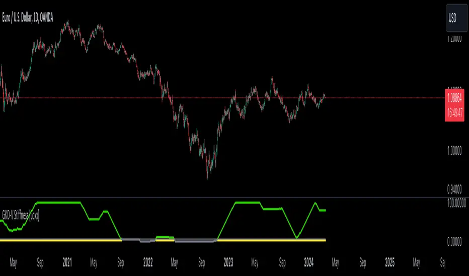
GKD-V Semi-Variance [Loxx]Giga Kaleidoscope Semi-Variance is a Volatility / Volume module included in Loxx's "Giga Kaleidoscope Modularized Trading System".
█ Giga Kaleidoscope Modularized Trading System
What is Loxx's "Giga Kaleidoscope Modularized Trading System"?
The Giga Kaleidoscope Modularized Trading System is a trading system built on the philosophy of the NNFX (No Nonsense Forex) algorithmic trading.
What is an NNFX algorithmic trading strategy?
The NNFX algorithm is built on the principles of trend, momentum, and volatility . There are six core components in the NNFX trading algorithm:
1. Volatility - price volatility ; e.g., Average True Range , True Range Double, Close-to-Close, etc.
2. Baseline - a moving average to identify price trend
3. Confirmation 1 - a technical indicator used to identify trends.
4. Confirmation 2 - a technical indicator used to identify trends.
5. Continuation - a technical indicator used to identify trends.
6. Volatility / Volume - a technical indicator used to identify volatility / volume breakouts/breakdown.
7. Exit - a technical indicator used to determine when a trend is exhausted.
How does Loxx's GKD (Giga Kaleidoscope Modularized Trading System) implement the NNFX algorithm outlined above?
Loxx's GKD v1.0 system has five types of modules (indicators/strategies). These modules are:
1. GKD-BT - Backtesting module (Volatility , Number 1 in the NNFX algorithm)
2. GKD-B - Baseline module (Baseline and Volatility / Volume , Numbers 1 and 2 in the NNFX algorithm)
3. GKD-C - Confirmation 1/2 and Continuation module (Confirmation 1/2 and Continuation, Numbers 3, 4, and 5 in the NNFX algorithm)
4. GKD-V - Volatility / Volume module (Confirmation 1/2, Number 6 in the NNFX algorithm)
5. GKD-E - Exit module (Exit, Number 7 in the NNFX algorithm)
(additional module types will added in future releases)
Each module interacts with every module by passing data between modules. Data is passed between each module as described below:
GKD-B => GKD-V => GKD-C(1) => GKD-C(2) => GKD-C(Continuation) => GKD-E => GKD-BT
That is, the Baseline indicator passes its data to Volatility / Volume . The Volatility / Volume indicator passes its values to the Confirmation 1 indicator. The Confirmation 1 indicator passes its values to the Confirmation 2 indicator. The Confirmation 2 indicator passes its values to the Continuation indicator. The Continuation indicator passes its values to the Exit indicator, and finally, the Exit indicator passes its values to the Backtest strategy.
This chaining of indicators requires that each module conform to Loxx's GKD protocol, therefore allowing for the testing of every possible combination of technical indicators that make up the six components of the NNFX algorithm.
What does the application of the GKD trading system look like?
Example trading system:
Backtest: Strategy with 1-3 take profits, trailing stop loss, multiple types of PnL volatility, and 2 backtesting styles
Baseline: Hull Moving Average
Volatility/Volume: Semi-variance as shown on the chart above
Confirmation 1: Halftrend Averages
Confirmation 2: Williams Percent Range
Continuation: Fisher Transform
Exit: Rex Oscillator
Each GKD indicator is denoted with a module identifier of either: GKD-BT, GKD-B, GKD-C, GKD-V, or GKD-E. This allows traders to understand to which module each indicator belongs and where each indicator fits into the GKD protocol chain.
Giga Kaleidoscope Modularized Trading System Signals (based on the NNFX algorithm)
Standard Entry
1. GKD-C Confirmation 1 Signal
2. GKD-B Baseline agrees
3. Price is within a range of 0.2x Volatility and 1.0x Volatility of the Goldie Locks Mean
4. GKD-C Confirmation 2 agrees
5. GKD-V Volatility / Volume agrees
Baseline Entry
1. GKD-B Baseline signal
2. GKD-C Confirmation 1 agrees
3. Price is within a range of 0.2x Volatility and 1.0x Volatility of the Goldie Locks Mean
4. GKD-C Confirmation 2 agrees
5. GKD-V Volatility / Volume agrees
6. GKD-C Confirmation 1 signal was less than 7 candles prior
Continuation Entry
1. Standard Entry, Baseline Entry, or Pullback; entry triggered previously
2. GKD-B Baseline hasn't crossed since entry signal trigger
3. GKD-C Confirmation Continuation Indicator signals
4. GKD-C Confirmation 1 agrees
5. GKD-B Baseline agrees
6. GKD-C Confirmation 2 agrees
1-Candle Rule Standard Entry
1. GKD-C Confirmation 1 signal
2. GKD-B Baseline agrees
3. Price is within a range of 0.2x Volatility and 1.0x Volatility of the Goldie Locks Mean
Next Candle:
1. Price retraced (Long: close < close or Short: close > close)
2. GKD-B Baseline agrees
3. GKD-C Confirmation 1 agrees
4. GKD-C Confirmation 2 agrees
5. GKD-V Volatility / Volume agrees
1-Candle Rule Baseline Entry
1. GKD-B Baseline signal
2. GKD-C Confirmation 1 agrees
3. Price is within a range of 0.2x Volatility and 1.0x Volatility of the Goldie Locks Mean
4. GKD-C Confirmation 1 signal was less than 7 candles prior
Next Candle:
1. Price retraced (Long: close < close or Short: close > close)
2. GKD-B Baseline agrees
3. GKD-C Confirmation 1 agrees
4. GKD-C Confirmation 2 agrees
5. GKD-V Volatility / Volume Agrees
PullBack Entry
1. GKD-B Baseline signal
2. GKD-C Confirmation 1 agrees
3. Price is beyond 1.0x Volatility of Baseline
Next Candle:
1. Price is within a range of 0.2x Volatility and 1.0x Volatility of the Goldie Locks Mean
3. GKD-C Confirmation 1 agrees
4. GKD-C Confirmation 2 agrees
5. GKD-V Volatility / Volume Agrees
█ Semi-Variance
What is Semi-Variance
Semi-variance is a statistical measure that represents the variability of returns in a financial portfolio or investment that fall below a certain threshold or benchmark return. Unlike traditional variance, which measures the dispersion of all returns, semi-variance only focuses on the downside risk or the deviation of returns that are below a specified target return.
Semi-variance is calculated as the average of the squared deviations of returns below the target return. It provides information on the risk of losing money and helps investors assess the stability and reliability of a portfolio or investment. A high semi-variance indicates a higher level of downside risk, while a low semi-variance suggests a lower level of downside risk.
In finance, semi-variance is often used in conjunction with other risk measures, such as standard deviation, beta, and value-at-risk, to give a comprehensive understanding of a portfolio's risk-return profile.
This indicator calculates the difference betwen upward volatility and downward volatility. You can choose between guassian normalized or regular.
Other things to note
The GKD trading system requires that a GKD-V indicator be present in the indicator chain, but the GKD-V indicator doesn't need to be active. You can turn on/off the Volatility Ratio as you wish so you can backtest your trading strategy with the filter on or off.
Additional features will be added in future releases.
Cari skrip untuk "Volatility"

GKD-V Loxx Volty [Loxx]Giga Kaleidoscope Loxx Volty is a Volatility/Volume module included in Loxx's "Giga Kaleidoscope Modularized Trading System".
█ Giga Kaleidoscope Modularized Trading System
What is Loxx's "Giga Kaleidoscope Modularized Trading System"?
The Giga Kaleidoscope Modularized Trading System is a trading system built on the philosophy of the NNFX (No Nonsense Forex) algorithmic trading.
What is an NNFX algorithmic trading strategy?
The NNFX algorithm is built on the principles of trend, momentum, and volatility. There are six core components in the NNFX trading algorithm:
1. Volatility - price volatility; e.g., Average True Range, True Range Double, Close-to-Close, etc.
2. Baseline - a moving average to identify price trend
3. Confirmation 1 - a technical indicator used to identify trends.
4. Confirmation 2 - a technical indicator used to identify trends.
5. Continuation - a technical indicator used to identify trends.
6. Volatility/Volume - a technical indicator used to identify volatility/volume breakouts/breakdown.
7. Exit - a technical indicator used to determine when a trend is exhausted.
How does Loxx's GKD (Giga Kaleidoscope Modularized Trading System) implement the NNFX algorithm outlined above?
Loxx's GKD v1.0 system has five types of modules (indicators/strategies). These modules are:
1. GKD-BT - Backtesting module (Volatility, Number 1 in the NNFX algorithm)
2. GKD-B - Baseline module (Baseline and Volatility/Volume, Numbers 1 and 2 in the NNFX algorithm)
3. GKD-C - Confirmation 1/2 and Continuation module (Confirmation 1/2 and Continuation, Numbers 3, 4, and 5 in the NNFX algorithm)
4. GKD-V - Volatility/Volume module (Confirmation 1/2, Number 6 in the NNFX algorithm)
5. GKD-E - Exit module (Exit, Number 7 in the NNFX algorithm)
(additional module types will added in future releases)
Each module interacts with every module by passing data between modules. Data is passed between each module as described below:
GKD-B => GKD-V => GKD-C(1) => GKD-C(2) => GKD-C(Continuation) => GKD-E => GKD-BT
That is, the Baseline indicator passes its data to Volatility/Volume. The Volatility/Volume indicator passes its values to the Confirmation 1 indicator. The Confirmation 1 indicator passes its values to the Confirmation 2 indicator. The Confirmation 2 indicator passes its values to the Continuation indicator. The Continuation indicator passes its values to the Exit indicator, and finally, the Exit indicator passes its values to the Backtest strategy.
This chaining of indicators requires that each module conform to Loxx's GKD protocol, therefore allowing for the testing of every possible combination of technical indicators that make up the six components of the NNFX algorithm.
What does the application of the GKD trading system look like?
Example trading system:
Backtest: Strategy with 1-3 take profits, trailing stop loss, multiple types of PnL volatility, and 2 backtesting styles
Baseline: Leader Exponential Moving Average
Volatility/Volume: Loxx Volty as shown on the chart above
Confirmation 1: Double Smoothed Stochastic of Momentum
Confirmation 2: Jurik Turning Point Oscillator
Continuation: Fisher Transform
Exit: Rex Oscillator
Each GKD indicator is denoted with a module identifier of either: GKD-BT, GKD-B, GKD-C, GKD-V, or GKD-E. This allows traders to understand to which module each indicator belongs and where each indicator fits into the GKD protocol chain.
Giga Kaleidoscope Modularized Trading System Signals (based on the NNFX algorithm)
Standard Entry
1. GKD-C Confirmation 1 Signal
2. GKD-B Baseline agrees
3. Price is within a range of 0.2x Volatility and 1.0x Volatility of the Goldie Locks Mean
4. GKD-C Confirmation 2 agrees
5. GKD-V Volatility/Volume agrees
Baseline Entry
1. GKD-B Baseline signal
2. GKD-C Confirmation 1 agrees
3. Price is within a range of 0.2x Volatility and 1.0x Volatility of the Goldie Locks Mean
4. GKD-C Confirmation 2 agrees
5. GKD-V Volatility/Volume agrees
6. GKD-C Confirmation 1 signal was less than 7 candles prior
Continuation Entry
1. Standard Entry, Baseline Entry, or Pullback; entry triggered previously
2. GKD-B Baseline hasn't crossed since entry signal trigger
3. GKD-C Confirmation Continuation Indicator signals
4. GKD-C Confirmation 1 agrees
5. GKD-B Baseline agrees
6. GKD-C Confirmation 2 agrees
1-Candle Rule Standard Entry
1. GKD-C Confirmation 1 signal
2. GKD-B Baseline agrees
3. Price is within a range of 0.2x Volatility and 1.0x Volatility of the Goldie Locks Mean
Next Candle:
1. Price retraced (Long: close < close or Short: close > close )
2. GKD-B Baseline agrees
3. GKD-C Confirmation 1 agrees
4. GKD-C Confirmation 2 agrees
5. GKD-V Volatility/Volume agrees
1-Candle Rule Baseline Entry
1. GKD-B Baseline signal
2. GKD-C Confirmation 1 agrees
3. Price is within a range of 0.2x Volatility and 1.0x Volatility of the Goldie Locks Mean
4. GKD-C Confirmation 1 signal was less than 7 candles prior
Next Candle:
1. Price retraced (Long: close < close or Short: close > close )
2. GKD-B Baseline agrees
3. GKD-C Confirmation 1 agrees
4. GKD-C Confirmation 2 agrees
5. GKD-V Volatility/Volume Agrees
PullBack Entry
1. GKD-B Baseline signal
2. GKD-C Confirmation 1 agrees
3. Price is beyond 1.0x Volatility of Baseline
Next Candle:
1. Price is within a range of 0.2x Volatility and 1.0x Volatility of the Goldie Locks Mean
3. GKD-C Confirmation 1 agrees
4. GKD-C Confirmation 2 agrees
5. GKD-V Volatility/Volume Agrees
█ Loxx Volty
What is Loxx Volty
One of the lesser known qualities of Loxx smoothing is that the Loxx smoothing process is adaptive. "Loxx Volty" (a sort of market volatility) is what makes Loxx smoothing adaptive. The Loxx Volty calculation can be used as both a standalone indicator and to smooth other indicators that you wish to make adaptive.
Other things to note
The GKD trading system requires that a GKD-V indicator be present in the indicator chain, but the GKD-V indicator doesn't need to be active. You can turn on/off the Volatility Ratio as you wish so you can backtest your trading strategy with the filter on or off.
Additional features will be added in future releases.
This indicator is only available to ALGX Trading VIP group members . You can see the Author's Instructions below to get more information on how to get access.

Hurst Exponent Adaptive Filter (HEAF) [PhenLabs]📊 PhenLabs - Hurst Exponent Adaptive Filter (HEAF)
Version: PineScript™ v6
📌 Description
The Hurst Exponent Adaptive Filter (HEAF) is an advanced Pine Script indicator designed to dynamically adjust moving average calculations based on real time market regimes detected through the Hurst Exponent. The intention behind the creation of this indicator was not a buy/sell indicator but rather a tool to help sharpen traders ability to distinguish regimes in the market mathematically rather than guessing. By analyzing price persistence, it identifies whether the market is trending, mean-reverting, or exhibiting random walk behavior, automatically adapting the MA length to provide more responsive alerts in volatile conditions and smoother outputs in stable ones. This helps traders avoid false signals in choppy markets and capitalize on strong trends, making it ideal for adaptive trading strategies across various timeframes and assets.
Unlike traditional moving averages, HEAF incorporates fractal dimension analysis via the Hurst Exponent to create a self-tuning filter that evolves with market conditions. Traders benefit from visual cues like color coded regimes, adaptive bands for volatility channels, and an information panel that suggests appropriate strategies, enhancing decision making without constant manual adjustments by the user.
🚀 Points of Innovation
Dynamic MA length adjustment using Hurst Exponent for regime-aware filtering, reducing lag in trends and noise in ranges.
Integrated market regime classification (trending, mean-reverting, random) with visual and alert-based notifications.
Customizable color themes and adaptive bands that incorporate ATR for volatility-adjusted channels.
Built-in information panel providing real-time strategy recommendations based on detected regimes.
Power sensitivity parameter to fine-tune adaptation aggressiveness, allowing personalization for different trading styles.
Support for multiple MA types (EMA, SMA, WMA) within an adaptive framework.
🔧 Core Components
Hurst Exponent Calculation: Computes the fractal dimension of price series over a user-defined lookback to detect market persistence or anti-persistence.
Adaptive Length Mechanism: Maps Hurst values to MA lengths between minimum and maximum bounds, using a power function for sensitivity control.
Moving Average Engine: Applies the chosen MA type (EMA, SMA, or WMA) to the adaptive length for the core filter line.
Adaptive Bands: Creates upper and lower channels using ATR multiplied by a band factor, scaled to the current adaptive length.
Regime Detection: Classifies market state with thresholds (e.g., >0.55 for trending) and triggers alerts on regime changes.
Visualization System: Includes gradient fills, regime-colored MA lines, and an info panel for at-a-glance insights.
🔥 Key Features
Regime-Adaptive Filtering: Automatically shortens MA in mean-reverting markets for quick responses and lengthens it in trends for smoother signals, helping traders stay aligned with market dynamics.
Custom Alerts: Notifies on regime shifts and band breakouts, enabling timely strategy adjustments like switching to trend-following in bullish regimes.
Visual Enhancements: Color-coded MA lines, gradient band fills, and an optional info panel that displays market state and trading tips, improving chart readability.
Flexible Settings: Adjustable lookback, min/max lengths, sensitivity power, MA type, and themes to suit various assets and timeframes.
Band Breakout Signals: Highlights potential overbought/oversold conditions via ATR-based channels, useful for entry/exit timing.
🎨 Visualization
Main Adaptive MA Line: Plotted with regime-based colors (e.g., green for trending) to visually indicate market state and filter position relative to price.
Adaptive Bands: Upper and lower lines with gradient fills between them, showing volatility channels that widen in random regimes and tighten in trends.
Price vs. MA Fills: Color-coded areas between price and MA (e.g., bullish green above MA in trending modes) for quick trend strength assessment.
Information Panel: Top-right table displaying current regime (e.g., "Trending Market") and strategy suggestions like "Follow trends" or "Trade ranges."
📖 Usage Guidelines
Core Settings
Hurst Lookback Period
Default: 100
Range: 20-500
Description: Sets the period for Hurst Exponent calculation; longer values provide more stable regime detection but may lag, while shorter ones are more responsive to recent changes.
Minimum MA Length
Default: 10
Range: 5-50
Description: Defines the shortest possible adaptive MA length, ideal for fast responses in mean-reverting conditions.
Maximum MA Length
Default: 200
Range: 50-500
Description: Sets the longest adaptive MA length for smoothing in strong trends; adjust based on asset volatility.
Sensitivity Power
Default: 2.0
Range: 1.0-5.0
Description: Controls how aggressively the length adapts to Hurst changes; higher values make it more sensitive to regime shifts.
MA Type
Default: EMA
Options: EMA, SMA, WMA
Description: Chooses the moving average calculation method; EMA is more responsive, while SMA/WMA offer different weighting.
🖼️ Visual Settings
Show Adaptive Bands
Default: True
Description: Toggles visibility of upper/lower bands for volatility channels.
Band Multiplier
Default: 1.5
Range: 0.5-3.0
Description: Scales band width using ATR; higher values create wider channels for conservative signals.
Show Information Panel
Default: True
Description: Displays regime info and strategy tips in a top-right panel.
MA Line Width
Default: 2
Range: 1-5
Description: Adjusts thickness of the main MA line for better visibility.
Color Theme
Default: Blue
Options: Blue, Classic, Dark Purple, Vibrant
Description: Selects color scheme for MA, bands, and fills to match user preferences.
🚨 Alert Settings
Enable Alerts
Default: True
Description: Activates notifications for regime changes and band breakouts.
✅ Best Use Cases
Trend-Following Strategies: In detected trending regimes, use the adaptive MA as a trailing stop or entry filter for momentum trades.
Range Trading: During mean-reverting periods, monitor band breakouts for buying dips or selling rallies within channels.
Risk Management in Random Markets: Reduce exposure when random walk is detected, using tight stops suggested in the info panel.
Multi-Timeframe Analysis: Apply on higher timeframes for regime confirmation, then drill down to lower ones for entries.
Volatility-Based Entries: Use upper/lower band crossovers as signals in adaptive channels for overbought/oversold trades.
⚠️ Limitations
Lagging in Transitions: Regime detection may delay during rapid market shifts, requiring confirmation from other tools.
Not a Standalone System: Best used in conjunction with other indicators; random regimes can lead to whipsaws if traded aggressively.
Parameter Sensitivity: Optimal settings vary by asset and timeframe, necessitating backtesting.
💡 What Makes This Unique
Hurst-Driven Adaptation: Unlike static MAs, it uses fractal analysis to self-tune, providing regime-specific filtering that's rare in standard indicators.
Integrated Strategy Guidance: The info panel offers actionable tips tied to regimes, bridging analysis and execution.
Multi-Regime Visualization: Combines adaptive bands, colored fills, and alerts in one tool for comprehensive market state awareness.
🔬 How It Works
Hurst Exponent Computation:
Calculates log returns over the lookback period to derive the rescaled range (R/S) ratio.
Normalizes to a 0-1 value, where >0.55 indicates trending, <0.45 mean-reverting, and in-between random.
Length Adaptation:
Maps normalized Hurst to an MA length via a power function, clamping between min and max.
Applies the selected MA type to close prices using this dynamic length.
Visualization and Signals:
Plots the MA with regime colors, adds ATR-based bands, and fills areas for trend strength.
Triggers alerts on regime changes or band crosses, with the info panel suggesting strategies like momentum riding in trends.
💡 Note:
For optimal results, backtest settings on your preferred assets and combine with volume or momentum indicators. Remember, no indicator guarantees profits—use with proper risk management. Access premium features and support at PhenLabs.

VIX Bars [CrossTrade]In simple terms, this indicator colors your chart bars based on the VIX levels. We know that high volatility is unstainable and will naturally regress to a calmer market, therefore highlighting the bars where VIX is at extreme highs can sometimes indicate a market turning point. Consider pairing this indicator with my VIX Heatmap indicator for a complete picture of volatility.
Customizable VIX Levels: You can set your own thresholds for when the bars turn green or red. Green bars pop up when the VIX is above your set upper level (default is 30) - kind of like a heads-up that things might get bumpy. Red bars show up when the VIX dips below your lower threshold (default is 15), signaling calmer waters.
Optional Donchian Channel Filter: The Donchian Channel filter looks at the highest highs and lowest lows over your chosen period (default's 52 days) and only colors the bars if they match the filter's criteria. This adds an extra layer of confirmation that the colored bars at at a major high or low.
Visual Simplicity: The indicator keeps things visually straightforward. No cluttered screen, just colored bars telling you a story about market vibes. Alert come standard to signal those potential bottom or top bars based on the VIX being at your preferred extreme levels.
In essence, "VIX Bars" is like having a volatility radar on your chart. It doesn't make predictions, but it sure gives you a neat, color-coded heads-up on market sentiment. Great for adding an extra dimension to your analysis without getting all tangled up in complex indicators!

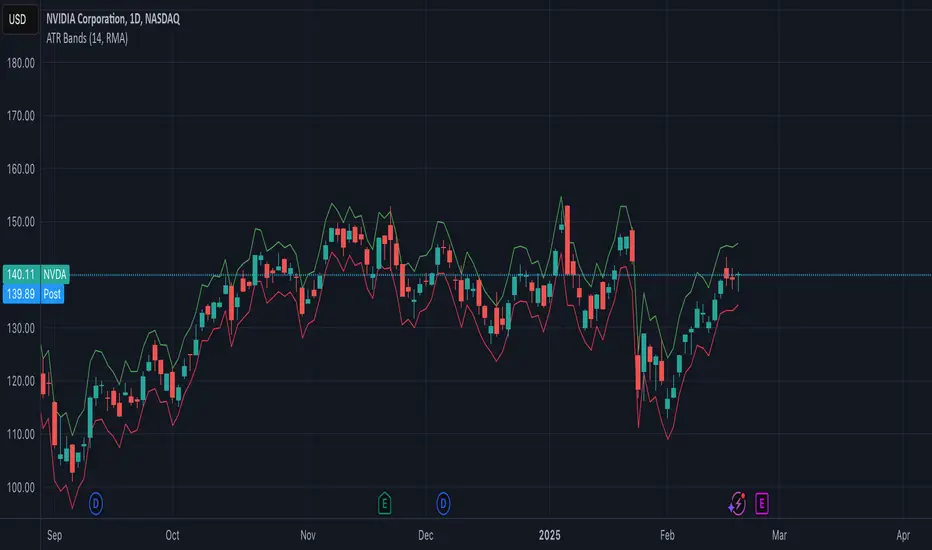
ATR BandsThe ATR Bands indicator is a volatility-based tool that plots dynamic support and resistance levels around the price using the Average True Range (ATR). It consists of two bands:
Upper Band: Calculated as current price + ATR, representing an upper volatility threshold.
Lower Band: Calculated as current price - ATR, serving as a lower volatility threshold.
Key Features:
✅ Measures Volatility: Expands and contracts based on market volatility.
✅ Dynamic Support & Resistance: Helps identify potential breakout or reversal zones.
✅ Customizable Smoothing: Supports multiple moving average methods (RMA, SMA, EMA, WMA) for ATR calculation.
How to Use:
Trend Confirmation: If the price consistently touches or exceeds the upper band, it may indicate strong bullish momentum.
Reversal Signals: A price approaching the lower band may suggest a potential reversal or increased selling pressure.
Volatility Assessment: Wide bands indicate high volatility, while narrow bands suggest consolidation.
This indicator is useful for traders looking to incorporate volatility-based strategies into their trading decisions
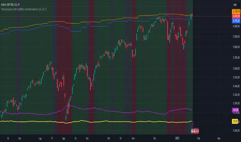
Trend Analysis with Volatility and MomentumVolatility and Momentum Trend Analyzer
The Volatility and Momentum Trend Analyzer is a multi-faceted TradingView indicator designed to provide a comprehensive analysis of market trends, volatility, and momentum. It incorporates key features to identify trend direction (uptrend, downtrend, or sideways), visualize weekly support and resistance levels, and offer a detailed assessment of market strength and activity. Below is a breakdown of its functionality:
1. Input Parameters
The indicator provides customizable settings for precision and adaptability:
Volatility Lookback Period: Configurable period (default: 14) for calculating Average True Range (ATR), which measures market volatility.
Momentum Lookback Period: Configurable period (default: 14) for calculating the Rate of Change (ROC), which measures the speed and strength of price movements.
Support/Resistance Lookback Period: Configurable period (default: 7 weeks) to determine critical support and resistance levels based on weekly high and low prices.
2. Volatility Analysis (ATR)
The Average True Range (ATR) is calculated to quantify the market's volatility:
What It Does: ATR measures the average range of price movement over the specified lookback period.
Visualization: Plotted as a purple line in a separate panel below the price chart, with values amplified (multiplied by 10) for better visibility.
3. Momentum Analysis (ROC)
The Rate of Change (ROC) evaluates the momentum of price movements:
What It Does: ROC calculates the percentage change in closing prices over the specified lookback period, indicating the strength and direction of market moves.
Visualization: Plotted as a yellow line in a separate panel below the price chart, with values amplified (multiplied by 10) for better visibility.
4. Trend Detection
The indicator identifies the current market trend based on momentum and the position of the price relative to its moving average:
Uptrend: Occurs when momentum is positive, and the closing price is above the simple moving average (SMA) of the specified lookback period.
Downtrend: Occurs when momentum is negative, and the closing price is below the SMA.
Sideways Trend: Occurs when neither of the above conditions is met.
Visualization: The background of the price chart changes color to reflect the detected trend:
Green: Uptrend.
Red: Downtrend.
Gray: Sideways trend.
5. Weekly Support and Resistance
Critical levels are calculated based on weekly high and low prices:
Support: The lowest price observed over the last specified number of weeks.
Resistance: The highest price observed over the last specified number of weeks.
Visualization:
Blue Line: Indicates the support level.
Orange Line: Indicates the resistance level.
Both lines are displayed on the main price chart, dynamically updating as new data becomes available.
6. Alerts
The indicator provides configurable alerts for trend changes, helping traders stay informed without constant monitoring:
Uptrend Alert: Notifies when the market enters an uptrend.
Downtrend Alert: Notifies when the market enters a downtrend.
Sideways Alert: Notifies when the market moves sideways.
7. Key Use Cases
Trend Following: Identify and follow the dominant trend to capitalize on sustained price movements.
Volatility Assessment: Measure market activity to determine potential breakouts or quiet consolidation phases.
Support and Resistance: Highlight key levels where price is likely to react, assisting in decision-making for entries, exits, or stop-loss placement.
Momentum Tracking: Gauge the strength and speed of price moves to validate trends or anticipate reversals.
8. Visualization Summary
Main Chart:
Background color-coded for trend direction (green, red, gray).
Blue and orange lines for weekly support and resistance.
Lower Panels:
Purple line for volatility (ATR).
Yellow line for momentum (ROC).
vol_rangesThis script shows three measures of volatility:
historical (hv): realized volatility of the recent past
median (mv): a long run average of realized volatility
implied (iv): a user-defined volatility
Historical and median volatility are based on the EWMA, rather than standard deviation, method of calculating volatility. Since Tradingview's built in ema function uses a window, the "window" parameter determines how much historical data is used to calculate these volatility measures. E.g. 30 on a daily chart means the previous 30 days.
The plots above and below historical candles show past projections based on these measures. The "periods to expiration" dictates how far the projection extends. At 30 periods to expiration (default), the plot will indicate the one standard deviation range from 30 periods ago. This is calculated by multiplying the volatility measure by the square root of time. For example, if the historical volatility (hv) was 20% and the window is 30, then the plot is drawn over: close * 1.2 * sqrt(30/252).
At the most recent candle, this same calculation is simply drawn as a line projecting into the future.
This script is intended to be used with a particular options contract in mind. For example, if the option expires in 15 days and has an implied volatility of 25%, choose 15 for the window and 25 for the implied volatility options. The ranges drawn will reflect the two standard deviation range both in the future (lines) and at any point in the past (plots) for HV (blue), MV (red), and IV (grey).

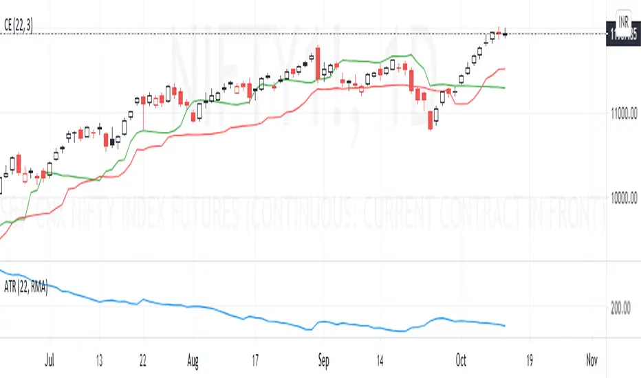
Chandelier ExitChandelier Exit (CE) is a volatility-based indicator developed by "Chuck Le Beau", ATR is used to measure the Volatility.
It identifies stop loss exit points for long and short trading positions.
Configuring the ATR period = 1 and Multiplier = (say) 1.25 or 1.5, it can be used for readily available buffer Stop Loss value from previous high/low.
Futures Beta Overview with Different BenchmarksBeta Trading and Its Implementation with Futures
Understanding Beta
Beta is a measure of a security's volatility in relation to the overall market. It represents the sensitivity of the asset's returns to movements in the market, typically benchmarked against an index like the S&P 500. A beta of 1 indicates that the asset moves in line with the market, while a beta greater than 1 suggests higher volatility and potential risk, and a beta less than 1 indicates lower volatility.
The Beta Trading Strategy
Beta trading involves creating positions that exploit the discrepancies between the theoretical (or expected) beta of an asset and its actual market performance. The strategy often includes:
Long Positions on High Beta Assets: Investors might take long positions in assets with high beta when they expect market conditions to improve, as these assets have the potential to generate higher returns.
Short Positions on Low Beta Assets: Conversely, shorting low beta assets can be a strategy when the market is expected to decline, as these assets tend to perform better in down markets compared to high beta assets.
Betting Against (Bad) Beta
The paper "Betting Against Beta" by Frazzini and Pedersen (2014) provides insights into a trading strategy that involves betting against high beta stocks in favor of low beta stocks. The authors argue that high beta stocks do not provide the expected return premium over time, and that low beta stocks can yield higher risk-adjusted returns.
Key Points from the Paper:
Risk Premium: The authors assert that investors irrationally demand a higher risk premium for holding high beta stocks, leading to an overpricing of these assets. Conversely, low beta stocks are often undervalued.
Empirical Evidence: The paper presents empirical evidence showing that portfolios of low beta stocks outperform portfolios of high beta stocks over long periods. The performance difference is attributed to the irrational behavior of investors who overvalue riskier assets.
Market Conditions: The paper suggests that the underperformance of high beta stocks is particularly pronounced during market downturns, making low beta stocks a more attractive investment during volatile periods.
Implementation of the Strategy with Futures
Futures contracts can be used to implement the betting against beta strategy due to their ability to provide leveraged exposure to various asset classes. Here’s how the strategy can be executed using futures:
Identify High and Low Beta Futures: The first step involves identifying futures contracts that have high beta characteristics (more sensitive to market movements) and those with low beta characteristics (less sensitive). For example, commodity futures like crude oil or agricultural products might exhibit high beta due to their price volatility, while Treasury bond futures might show lower beta.
Construct a Portfolio: Investors can construct a portfolio that goes long on low beta futures and short on high beta futures. This can involve trading contracts on stock indices for high beta stocks and bonds for low beta exposures.
Leverage and Risk Management: Futures allow for leverage, which means that a small movement in the underlying asset can lead to significant gains or losses. Proper risk management is essential, using stop-loss orders and position sizing to mitigate the inherent risks associated with leveraged trading.
Adjusting Positions: The positions may need to be adjusted based on market conditions and the ongoing performance of the futures contracts. Continuous monitoring and rebalancing of the portfolio are essential to maintain the desired risk profile.
Performance Evaluation: Finally, investors should regularly evaluate the performance of the portfolio to ensure it aligns with the expected outcomes of the betting against beta strategy. Metrics like the Sharpe ratio can be used to assess the risk-adjusted returns of the portfolio.
Conclusion
Beta trading, particularly the strategy of betting against high beta assets, presents a compelling approach to capitalizing on market inefficiencies. The research by Frazzini and Pedersen emphasizes the benefits of focusing on low beta assets, which can yield more favorable risk-adjusted returns over time. When implemented using futures, this strategy can provide a flexible and efficient means to execute trades while managing risks effectively.
References
Frazzini, A., & Pedersen, L. H. (2014). Betting against beta. Journal of Financial Economics, 111(1), 1-25.
Fama, E. F., & French, K. R. (1992). The cross-section of expected stock returns. Journal of Finance, 47(2), 427-465.
Black, F. (1972). Capital Market Equilibrium with Restricted Borrowing. Journal of Business, 45(3), 444-454.
Ang, A., & Chen, J. (2010). Asymmetric volatility: Evidence from the stock and bond markets. Journal of Financial Economics, 99(1), 60-80.
By utilizing the insights from academic literature and implementing a disciplined trading strategy, investors can effectively navigate the complexities of beta trading in the futures market.

Average True Range with EMAIncreasing and decreasing volatility in respect to ATR crossing an ema of ATR.
Ema acts as a proxy for look-back period as per Historical Volatility Percentile.
ATR is a proxy for Volatility as per standard deviation.
Divergence below ema means low volatility: the more divergence, the lower.
Divergence above the ema means high volatility.

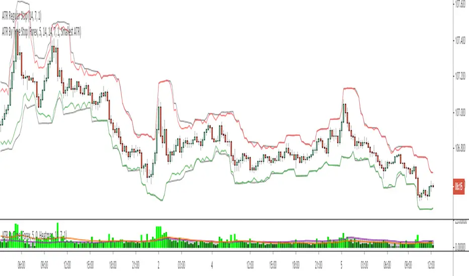
ATR By Time [Chart]What is ATR By Time (Chart)?
This premium indicator is a companion script to my ATR By Time indicator.
This companion script draws your stop loss price to the chart directly. In the above example, the black line represents a regular 1x ATR stop loss above and below price action, while the colored lines are the 1x ATR By Time indicator values when set to use the "Smallest ATR" in the settings menu.
When set to "Smallest ATR", the script calculates the regular ATR and the ATR By Time of Day and compares the distance of the two values. It then selects whichever value is smaller to be used as the stop loss, and adds or subtracts it to the most recent swing high or low (or the closing price if desired).
This allows for tighter stops and larger position sizing during certain times of day for aggressive traders when set to Smallest ATR, or wider stop losses during more volatile periods of the day for conservative traders when set to Largest ATR.
Stop Loss Distance Options:
- Regular ATR
- ATR By Time
- Smallest ATR
- Largest ATR
More Information
Similar to my RVOL By Time indicator, the ATR By Time indicator works on any market that has consistent trading session lengths . So it works best on Forex & Crypto, but also works on some Stock and Futures markets.
Instead of calculating the ATR based on recent price data like the regular ATR indicator, it calculates an ATR value for each candle based on that candle’s time of day .
For example, if you set the Lookback setting on this indicator to 14, then instead of calculating the ATR based on the past 14 candles, it will calculate an ATR value based on the past 14 trading sessions for each candle (as an average).
So in other words, your 10:00AM candle will show the average of the past 14 10:00AM candles rather than the past 14 candles leading up to that 10:00AM candle.
This is extremely useful for day traders in particular as it allows you to gauge the average range of candles during certain times of day instead of only by the most recent price action.
It also draws a regular ATR (optional) – so this is essentially an enhanced ATR script that gives you multiple readings on price volatility.
If you are interested in trying the script or you want more information on how the script works, there is more information available on my website including instructions on how to apply for a free trial: ATR By Time Feature Page .
Good luck with your trading!
Volatility Risk PremiumTHE INSURANCE PREMIUM OF THE STOCK MARKET
Every day, millions of investors face a fundamental question that has puzzled economists for decades: how much should protection against market crashes cost? The answer lies in a phenomenon called the Volatility Risk Premium, and understanding it may fundamentally change how you interpret market conditions.
Think of the stock market like a neighborhood where homeowners buy insurance against fire. The insurance company charges premiums based on their estimates of fire risk. But here is the interesting part: insurance companies systematically charge more than the actual expected losses. This difference between what people pay and what actually happens is the insurance premium. The same principle operates in financial markets, but instead of fire insurance, investors buy protection against market volatility through options contracts.
The Volatility Risk Premium, or VRP, measures exactly this difference. It represents the gap between what the market expects volatility to be (implied volatility, as reflected in options prices) and what volatility actually turns out to be (realized volatility, calculated from actual price movements). This indicator quantifies that gap and transforms it into actionable intelligence.
THE FOUNDATION
The academic study of volatility risk premiums began gaining serious traction in the early 2000s, though the phenomenon itself had been observed by practitioners for much longer. Three research papers form the backbone of this indicator's methodology.
Peter Carr and Liuren Wu published their seminal work "Variance Risk Premiums" in the Review of Financial Studies in 2009. Their research established that variance risk premiums exist across virtually all asset classes and persist over time. They documented that on average, implied volatility exceeds realized volatility by approximately three to four percentage points annualized. This is not a small number. It means that sellers of volatility insurance have historically collected a substantial premium for bearing this risk.
Tim Bollerslev, George Tauchen, and Hao Zhou extended this research in their 2009 paper "Expected Stock Returns and Variance Risk Premia," also published in the Review of Financial Studies. Their critical contribution was demonstrating that the VRP is a statistically significant predictor of future equity returns. When the VRP is high, meaning investors are paying substantial premiums for protection, future stock returns tend to be positive. When the VRP collapses or turns negative, it often signals that realized volatility has spiked above expectations, typically during market stress periods.
Gurdip Bakshi and Nikunj Kapadia provided additional theoretical grounding in their 2003 paper "Delta-Hedged Gains and the Negative Market Volatility Risk Premium." They demonstrated through careful empirical analysis why volatility sellers are compensated: the risk is not diversifiable and tends to materialize precisely when investors can least afford losses.
HOW THE INDICATOR CALCULATES VOLATILITY
The calculation begins with two separate measurements that must be compared: implied volatility and realized volatility.
For implied volatility, the indicator uses the CBOE Volatility Index, commonly known as the VIX. The VIX represents the market's expectation of 30-day forward volatility on the S&P 500, calculated from a weighted average of out-of-the-money put and call options. It is often called the "fear gauge" because it rises when investors rush to buy protective options.
Realized volatility requires more careful consideration. The indicator offers three distinct calculation methods, each with specific advantages rooted in academic literature.
The Close-to-Close method is the most straightforward approach. It calculates the standard deviation of logarithmic daily returns over a specified lookback period, then annualizes this figure by multiplying by the square root of 252, the approximate number of trading days in a year. This method is intuitive and widely used, but it only captures information from closing prices and ignores intraday price movements.
The Parkinson estimator, developed by Michael Parkinson in 1980, improves efficiency by incorporating high and low prices. The mathematical formula calculates variance as the sum of squared log ratios of daily highs to lows, divided by four times the natural logarithm of two, times the number of observations. This estimator is theoretically about five times more efficient than the close-to-close method because high and low prices contain additional information about the volatility process.
The Garman-Klass estimator, published by Mark Garman and Michael Klass in 1980, goes further by incorporating opening, high, low, and closing prices. The formula combines half the squared log ratio of high to low prices minus a factor involving the log ratio of close to open. This method achieves the minimum variance among estimators using only these four price points, making it particularly valuable for markets where intraday information is meaningful.
THE CORE VRP CALCULATION
Once both volatility measures are obtained, the VRP calculation is straightforward: subtract realized volatility from implied volatility. A positive result means the market is paying a premium for volatility insurance. A negative result means realized volatility has exceeded expectations, typically indicating market stress.
The raw VRP signal receives slight smoothing through an exponential moving average to reduce noise while preserving responsiveness. The default smoothing period of five days balances signal clarity against lag.
INTERPRETING THE REGIMES
The indicator classifies market conditions into five distinct regimes based on VRP levels.
The EXTREME regime occurs when VRP exceeds ten percentage points. This represents an unusual situation where the gap between implied and realized volatility is historically wide. Markets are pricing in significantly more fear than is materializing. Research suggests this often precedes positive equity returns as the premium normalizes.
The HIGH regime, between five and ten percentage points, indicates elevated risk aversion. Investors are paying above-average premiums for protection. This often occurs after market corrections when fear remains elevated but realized volatility has begun subsiding.
The NORMAL regime covers VRP between zero and five percentage points. This represents the long-term average state of markets where implied volatility modestly exceeds realized volatility. The insurance premium is being collected at typical rates.
The LOW regime, between negative two and zero percentage points, suggests either unusual complacency or that realized volatility is catching up to implied volatility. The premium is shrinking, which can precede either calm continuation or increased stress.
The NEGATIVE regime occurs when realized volatility exceeds implied volatility. This is relatively rare and typically indicates active market stress. Options were priced for less volatility than actually occurred, meaning volatility sellers are experiencing losses. Historically, deeply negative VRP readings have often coincided with market bottoms, though timing the reversal remains challenging.
TERM STRUCTURE ANALYSIS
Beyond the basic VRP calculation, sophisticated market participants analyze how volatility behaves across different time horizons. The indicator calculates VRP using both short-term (default ten days) and long-term (default sixty days) realized volatility windows.
Under normal market conditions, short-term realized volatility tends to be lower than long-term realized volatility. This produces what traders call contango in the term structure, analogous to futures markets where later delivery dates trade at premiums. The RV Slope metric quantifies this relationship.
When markets enter stress periods, the term structure often inverts. Short-term realized volatility spikes above long-term realized volatility as markets experience immediate turmoil. This backwardation condition serves as an early warning signal that current volatility is elevated relative to historical norms.
The academic foundation for term structure analysis comes from Scott Mixon's 2007 paper "The Implied Volatility Term Structure" in the Journal of Derivatives, which documented the predictive power of term structure dynamics.
MEAN REVERSION CHARACTERISTICS
One of the most practically useful properties of the VRP is its tendency to mean-revert. Extreme readings, whether high or low, tend to normalize over time. This creates opportunities for systematic trading strategies.
The indicator tracks VRP in statistical terms by calculating its Z-score relative to the trailing one-year distribution. A Z-score above two indicates that current VRP is more than two standard deviations above its mean, a statistically unusual condition. Similarly, a Z-score below negative two indicates VRP is unusually low.
Mean reversion signals trigger when VRP reaches extreme Z-score levels and then shows initial signs of reversal. A buy signal occurs when VRP recovers from oversold conditions (Z-score below negative two and rising), suggesting that the period of elevated realized volatility may be ending. A sell signal occurs when VRP contracts from overbought conditions (Z-score above two and falling), suggesting the fear premium may be excessive and due for normalization.
These signals should not be interpreted as standalone trading recommendations. They indicate probabilistic conditions based on historical patterns. Market context and other factors always matter.
MOMENTUM ANALYSIS
The rate of change in VRP carries its own information content. Rapidly rising VRP suggests fear is building faster than volatility is materializing, often seen in the early stages of corrections before realized volatility catches up. Rapidly falling VRP indicates either calming conditions or rising realized volatility eating into the premium.
The indicator tracks VRP momentum as the difference between current VRP and VRP from a specified number of bars ago. Positive momentum with positive acceleration suggests strengthening risk aversion. Negative momentum with negative acceleration suggests intensifying stress or rapid normalization from elevated levels.
PRACTICAL APPLICATION
For equity investors, the VRP provides context for risk management decisions. High VRP environments historically favor equity exposure because the market is pricing in more pessimism than typically materializes. Low or negative VRP environments suggest either reducing exposure or hedging, as markets may be underpricing risk.
For options traders, understanding VRP is fundamental to strategy selection. Strategies that sell volatility, such as covered calls, cash-secured puts, or iron condors, tend to profit when VRP is elevated and compress toward its mean. Strategies that buy volatility tend to profit when VRP is low and risk materializes.
For systematic traders, VRP provides a regime filter for other strategies. Momentum strategies may benefit from different parameters in high versus low VRP environments. Mean reversion strategies in VRP itself can form the basis of a complete trading system.
LIMITATIONS AND CONSIDERATIONS
No indicator provides perfect foresight, and the VRP is no exception. Several limitations deserve attention.
The VRP measures a relationship between two estimates, each subject to measurement error. The VIX represents expectations that may prove incorrect. Realized volatility calculations depend on the chosen method and lookback period.
Mean reversion tendencies hold over longer time horizons but provide limited guidance for short-term timing. VRP can remain extreme for extended periods, and mean reversion signals can generate losses if the extremity persists or intensifies.
The indicator is calibrated for equity markets, specifically the S&P 500. Application to other asset classes requires recalibration of thresholds and potentially different data sources.
Historical relationships between VRP and subsequent returns, while statistically robust, do not guarantee future performance. Structural changes in markets, options pricing, or investor behavior could alter these dynamics.
STATISTICAL OUTPUTS
The indicator presents comprehensive statistics including current VRP level, implied volatility from VIX, realized volatility from the selected method, current regime classification, number of bars in the current regime, percentile ranking over the lookback period, Z-score relative to recent history, mean VRP over the lookback period, realized volatility term structure slope, VRP momentum, mean reversion signal status, and overall market bias interpretation.
Color coding throughout the indicator provides immediate visual interpretation. Green tones indicate elevated VRP associated with fear and potential opportunity. Red tones indicate compressed or negative VRP associated with complacency or active stress. Neutral tones indicate normal market conditions.
ALERT CONDITIONS
The indicator provides alerts for regime transitions, extreme statistical readings, term structure inversions, mean reversion signals, and momentum shifts. These can be configured through the TradingView alert system for real-time monitoring across multiple timeframes.
REFERENCES
Bakshi, G., and Kapadia, N. (2003). Delta-Hedged Gains and the Negative Market Volatility Risk Premium. Review of Financial Studies, 16(2), 527-566.
Bollerslev, T., Tauchen, G., and Zhou, H. (2009). Expected Stock Returns and Variance Risk Premia. Review of Financial Studies, 22(11), 4463-4492.
Carr, P., and Wu, L. (2009). Variance Risk Premiums. Review of Financial Studies, 22(3), 1311-1341.
Garman, M. B., and Klass, M. J. (1980). On the Estimation of Security Price Volatilities from Historical Data. Journal of Business, 53(1), 67-78.
Mixon, S. (2007). The Implied Volatility Term Structure of Stock Index Options. Journal of Empirical Finance, 14(3), 333-354.
Parkinson, M. (1980). The Extreme Value Method for Estimating the Variance of the Rate of Return. Journal of Business, 53(1), 61-65.

Ultimate Moving Average Bands [CC+RedK]The Ultimate Moving Average Bands were created by me and @RedKTrader and this converts our Ultimate Moving Average into volatility bands that use the same adaptive logic to create the bands. I have enabled everything to be fully adjustable so please let me know if you find a more useful setting than what I have here by default. I'm sure everyone is familiar with volatility bands but generally speaking if a price goes above the volatility bands then this is either a sign of an extremely strong uptrend or a potential reversal point and vice versa. I have included strong buy and sell signals in addition to normal ones so darker colors are strong signals and lighter colors are normal ones. Buy when the lines turn green and sell when they turn red.
Let me know if there are any other scripts you would like to see me publish!

Volatility MeterThis is my third published indicator; its simple, but don't underestimate it. As the name suggests, it measures volatility. Specifically, it measures this through the incremental difference in closing prices. It then uses an SMA to smooth out the indicator's values, this will allow the trader to see the trend in volatility: Is it increasing? decreasing? etc.
If you have any thoughts or ideas about changing the indicator, let me know.
-racer8

GKD-V Stiffness [Loxx]The Giga Kaleidoscope GKD-V Stiffness is a Volume/Volatility module included in Loxx's "Giga Kaleidoscope Modularized Trading System."
█ GKD-V Stiffness
The stiffness indicator quantifies the market's momentum by analyzing the relationship between price movements and volatility over a specific time frame. It employs a moving average to smooth out price data, providing a baseline for trend assessment. The key element in this calculation is the incorporation of a volatility factor, typically standard deviation, which adjusts the moving average to account for market volatility. This adjusted moving average creates a benchmark that the current price must surpass to signal significant momentum.
By comparing the current price to this volatility-adjusted moving average, the stiffness indicator determines the strength of the market's trend. A higher stiffness value, surpassing a predefined threshold, indicates a strong and potentially profitable trend, either upward or downward, suggesting opportunities for strategic trading positions. Conversely, a stiffness value below the threshold signifies insufficient momentum, advising traders to refrain from entering the market due to the high risk of unpredictability. This method provides a systematic approach to evaluate market trends, enabling traders to make decisions based on the robustness of price movements relative to historical volatility.
█ Giga Kaleidoscope Modularized Trading System
Core components of an NNFX algorithmic trading strategy
The NNFX algorithm is built on the principles of trend, momentum, and volatility. There are six core components in the NNFX trading algorithm:
1. Volatility - price volatility; e.g., Average True Range, True Range Double, Close-to-Close, etc.
2. Baseline - a moving average to identify price trend
3. Confirmation 1 - a technical indicator used to identify trends
4. Confirmation 2 - a technical indicator used to identify trends
5. Continuation - a technical indicator used to identify trends
6. Volatility/Volume - a technical indicator used to identify volatility/volume breakouts/breakdown
7. Exit - a technical indicator used to determine when a trend is exhausted
8. Metamorphosis - a technical indicator that produces a compound signal from the combination of other GKD indicators*
*(not part of the NNFX algorithm)
What is Volatility in the NNFX trading system?
In the NNFX (No Nonsense Forex) trading system, ATR (Average True Range) is typically used to measure the volatility of an asset. It is used as a part of the system to help determine the appropriate stop loss and take profit levels for a trade. ATR is calculated by taking the average of the true range values over a specified period.
True range is calculated as the maximum of the following values:
-Current high minus the current low
-Absolute value of the current high minus the previous close
-Absolute value of the current low minus the previous close
ATR is a dynamic indicator that changes with changes in volatility. As volatility increases, the value of ATR increases, and as volatility decreases, the value of ATR decreases. By using ATR in NNFX system, traders can adjust their stop loss and take profit levels according to the volatility of the asset being traded. This helps to ensure that the trade is given enough room to move, while also minimizing potential losses.
Other types of volatility include True Range Double (TRD), Close-to-Close, and Garman-Klass
What is a Baseline indicator?
The baseline is essentially a moving average, and is used to determine the overall direction of the market.
The baseline in the NNFX system is used to filter out trades that are not in line with the long-term trend of the market. The baseline is plotted on the chart along with other indicators, such as the Moving Average (MA), the Relative Strength Index (RSI), and the Average True Range (ATR).
Trades are only taken when the price is in the same direction as the baseline. For example, if the baseline is sloping upwards, only long trades are taken, and if the baseline is sloping downwards, only short trades are taken. This approach helps to ensure that trades are in line with the overall trend of the market, and reduces the risk of entering trades that are likely to fail.
By using a baseline in the NNFX system, traders can have a clear reference point for determining the overall trend of the market, and can make more informed trading decisions. The baseline helps to filter out noise and false signals, and ensures that trades are taken in the direction of the long-term trend.
What is a Confirmation indicator?
Confirmation indicators are technical indicators that are used to confirm the signals generated by primary indicators. Primary indicators are the core indicators used in the NNFX system, such as the Average True Range (ATR), the Moving Average (MA), and the Relative Strength Index (RSI).
The purpose of the confirmation indicators is to reduce false signals and improve the accuracy of the trading system. They are designed to confirm the signals generated by the primary indicators by providing additional information about the strength and direction of the trend.
Some examples of confirmation indicators that may be used in the NNFX system include the Bollinger Bands, the MACD (Moving Average Convergence Divergence), and the MACD Oscillator. These indicators can provide information about the volatility, momentum, and trend strength of the market, and can be used to confirm the signals generated by the primary indicators.
In the NNFX system, confirmation indicators are used in combination with primary indicators and other filters to create a trading system that is robust and reliable. By using multiple indicators to confirm trading signals, the system aims to reduce the risk of false signals and improve the overall profitability of the trades.
What is a Continuation indicator?
In the NNFX (No Nonsense Forex) trading system, a continuation indicator is a technical indicator that is used to confirm a current trend and predict that the trend is likely to continue in the same direction. A continuation indicator is typically used in conjunction with other indicators in the system, such as a baseline indicator, to provide a comprehensive trading strategy.
What is a Volatility/Volume indicator?
Volume indicators, such as the On Balance Volume (OBV), the Chaikin Money Flow (CMF), or the Volume Price Trend (VPT), are used to measure the amount of buying and selling activity in a market. They are based on the trading volume of the market, and can provide information about the strength of the trend. In the NNFX system, volume indicators are used to confirm trading signals generated by the Moving Average and the Relative Strength Index. Volatility indicators include Average Direction Index, Waddah Attar, and Volatility Ratio. In the NNFX trading system, volatility is a proxy for volume and vice versa.
By using volume indicators as confirmation tools, the NNFX trading system aims to reduce the risk of false signals and improve the overall profitability of trades. These indicators can provide additional information about the market that is not captured by the primary indicators, and can help traders to make more informed trading decisions. In addition, volume indicators can be used to identify potential changes in market trends and to confirm the strength of price movements.
What is an Exit indicator?
The exit indicator is used in conjunction with other indicators in the system, such as the Moving Average (MA), the Relative Strength Index (RSI), and the Average True Range (ATR), to provide a comprehensive trading strategy.
The exit indicator in the NNFX system can be any technical indicator that is deemed effective at identifying optimal exit points. Examples of exit indicators that are commonly used include the Parabolic SAR, and the Average Directional Index (ADX).
The purpose of the exit indicator is to identify when a trend is likely to reverse or when the market conditions have changed, signaling the need to exit a trade. By using an exit indicator, traders can manage their risk and prevent significant losses.
In the NNFX system, the exit indicator is used in conjunction with a stop loss and a take profit order to maximize profits and minimize losses. The stop loss order is used to limit the amount of loss that can be incurred if the trade goes against the trader, while the take profit order is used to lock in profits when the trade is moving in the trader's favor.
Overall, the use of an exit indicator in the NNFX trading system is an important component of a comprehensive trading strategy. It allows traders to manage their risk effectively and improve the profitability of their trades by exiting at the right time.
What is an Metamorphosis indicator?
The concept of a metamorphosis indicator involves the integration of two or more GKD indicators to generate a compound signal. This is achieved by evaluating the accuracy of each indicator and selecting the signal from the indicator with the highest accuracy. As an illustration, let's consider a scenario where we calculate the accuracy of 10 indicators and choose the signal from the indicator that demonstrates the highest accuracy.
The resulting output from the metamorphosis indicator can then be utilized in a GKD-BT backtest by occupying a slot that aligns with the purpose of the metamorphosis indicator. The slot can be a GKD-B, GKD-C, or GKD-E slot, depending on the specific requirements and objectives of the indicator. This allows for seamless integration and utilization of the compound signal within the GKD-BT framework.
How does Loxx's GKD (Giga Kaleidoscope Modularized Trading System) implement the NNFX algorithm outlined above?
Loxx's GKD v2.0 system has five types of modules (indicators/strategies). These modules are:
1. GKD-BT - Backtesting module (Volatility, Number 1 in the NNFX algorithm)
2. GKD-B - Baseline module (Baseline and Volatility/Volume, Numbers 1 and 2 in the NNFX algorithm)
3. GKD-C - Confirmation 1/2 and Continuation module (Confirmation 1/2 and Continuation, Numbers 3, 4, and 5 in the NNFX algorithm)
4. GKD-V - Volatility/Volume module (Confirmation 1/2, Number 6 in the NNFX algorithm)
5. GKD-E - Exit module (Exit, Number 7 in the NNFX algorithm)
6. GKD-M - Metamorphosis module (Metamorphosis, Number 8 in the NNFX algorithm, but not part of the NNFX algorithm)
(additional module types will added in future releases)
Each module interacts with every module by passing data to A backtest module wherein the various components of the GKD system are combined to create a trading signal.
That is, the Baseline indicator passes its data to Volatility/Volume. The Volatility/Volume indicator passes its values to the Confirmation 1 indicator. The Confirmation 1 indicator passes its values to the Confirmation 2 indicator. The Confirmation 2 indicator passes its values to the Continuation indicator. The Continuation indicator passes its values to the Exit indicator, and finally, the Exit indicator passes its values to the Backtest strategy.
This chaining of indicators requires that each module conform to Loxx's GKD protocol, therefore allowing for the testing of every possible combination of technical indicators that make up the six components of the NNFX algorithm.
What does the application of the GKD trading system look like?
Example trading system:
Backtest: Multi-Ticker CC Backtest
Baseline: Hull Moving Average
Volatility/Volume: Hurst Exponent
Confirmation 1: Advance Trend Pressure as shown on the chart above
Confirmation 2: uf2018
Continuation: Coppock Curve
Exit: Rex Oscillator
Metamorphosis: Baseline Optimizer
Each GKD indicator is denoted with a module identifier of either: GKD-BT, GKD-B, GKD-C, GKD-V, GKD-M, or GKD-E. This allows traders to understand to which module each indicator belongs and where each indicator fits into the GKD system.
█ Giga Kaleidoscope Modularized Trading System Signals
Standard Entry
1. GKD-C Confirmation gives signal
2. Baseline agrees
3. Price inside Goldie Locks Zone Minimum
4. Price inside Goldie Locks Zone Maximum
5. Confirmation 2 agrees
6. Volatility/Volume agrees
1-Candle Standard Entry
1a. GKD-C Confirmation gives signal
2a. Baseline agrees
3a. Price inside Goldie Locks Zone Minimum
4a. Price inside Goldie Locks Zone Maximum
Next Candle
1b. Price retraced
2b. Baseline agrees
3b. Confirmation 1 agrees
4b. Confirmation 2 agrees
5b. Volatility/Volume agrees
Baseline Entry
1. GKD-B Baseline gives signal
2. Confirmation 1 agrees
3. Price inside Goldie Locks Zone Minimum
4. Price inside Goldie Locks Zone Maximum
5. Confirmation 2 agrees
6. Volatility/Volume agrees
7. Confirmation 1 signal was less than 'Maximum Allowable PSBC Bars Back' prior
1-Candle Baseline Entry
1a. GKD-B Baseline gives signal
2a. Confirmation 1 agrees
3a. Price inside Goldie Locks Zone Minimum
4a. Price inside Goldie Locks Zone Maximum
5a. Confirmation 1 signal was less than 'Maximum Allowable PSBC Bars Back' prior
Next Candle
1b. Price retraced
2b. Baseline agrees
3b. Confirmation 1 agrees
4b. Confirmation 2 agrees
5b. Volatility/Volume agrees
Volatility/Volume Entry
1. GKD-V Volatility/Volume gives signal
2. Confirmation 1 agrees
3. Price inside Goldie Locks Zone Minimum
4. Price inside Goldie Locks Zone Maximum
5. Confirmation 2 agrees
6. Baseline agrees
7. Confirmation 1 signal was less than 7 candles prior
1-Candle Volatility/Volume Entry
1a. GKD-V Volatility/Volume gives signal
2a. Confirmation 1 agrees
3a. Price inside Goldie Locks Zone Minimum
4a. Price inside Goldie Locks Zone Maximum
5a. Confirmation 1 signal was less than 'Maximum Allowable PSVVC Bars Back' prior
Next Candle
1b. Price retraced
2b. Volatility/Volume agrees
3b. Confirmation 1 agrees
4b. Confirmation 2 agrees
5b. Baseline agrees
Confirmation 2 Entry
1. GKD-C Confirmation 2 gives signal
2. Confirmation 1 agrees
3. Price inside Goldie Locks Zone Minimum
4. Price inside Goldie Locks Zone Maximum
5. Volatility/Volume agrees
6. Baseline agrees
7. Confirmation 1 signal was less than 7 candles prior
1-Candle Confirmation 2 Entry
1a. GKD-C Confirmation 2 gives signal
2a. Confirmation 1 agrees
3a. Price inside Goldie Locks Zone Minimum
4a. Price inside Goldie Locks Zone Maximum
5a. Confirmation 1 signal was less than 'Maximum Allowable PSC2C Bars Back' prior
Next Candle
1b. Price retraced
2b. Confirmation 2 agrees
3b. Confirmation 1 agrees
4b. Volatility/Volume agrees
5b. Baseline agrees
PullBack Entry
1a. GKD-B Baseline gives signal
2a. Confirmation 1 agrees
3a. Price is beyond 1.0x Volatility of Baseline
Next Candle
1b. Price inside Goldie Locks Zone Minimum
2b. Price inside Goldie Locks Zone Maximum
3b. Confirmation 1 agrees
4b. Confirmation 2 agrees
5b. Volatility/Volume agrees
Continuation Entry
1. Standard Entry, 1-Candle Standard Entry, Baseline Entry, 1-Candle Baseline Entry, Volatility/Volume Entry, 1-Candle Volatility/Volume Entry, Confirmation 2 Entry, 1-Candle Confirmation 2 Entry, or Pullback entry triggered previously
2. Baseline hasn't crossed since entry signal trigger
4. Confirmation 1 agrees
5. Baseline agrees
6. Confirmation 2 agrees
VolatilityCone by ImpliedVolatilityThis volatility cone draws the implied volatility as standard deviations from a measurement date.
For best results set measurement date to high volume bars.
How to use:
1) Select VolatilityCone from Indicators
2) Click to the chart to set the measurement date
3) Determine the impliedvolatility for the measurement date of your symbol
e.g.
For S&P500 use VIX value at measurement date for implied volatility

ER-Adaptive ATR, STD-Adaptive Damiani Volatmeter [Loxx]ER-Adaptive ATR, STD-Adaptive Damiani Volatmeter is a Damiani Volatmeter with both Efficiency-Ratio Adaptive ATR, used in place of ATR, and Adaptive Deviation, used in place of Standard Deviation.
What is Adaptive Deviation?
By definition, the Standard Deviation (STD, also represented by the Greek letter sigma σ or the Latin letter s) is a measure that is used to quantify the amount of variation or dispersion of a set of data values. In technical analysis we usually use it to measure the level of current volatility .
Standard Deviation is based on Simple Moving Average calculation for mean value. This version of standard deviation uses the properties of EMA to calculate what can be called a new type of deviation, and since it is based on EMA , we can call it EMA deviation. And added to that, Perry Kaufman's efficiency ratio is used to make it adaptive (since all EMA type calculations are nearly perfect for adapting).
The difference when compared to standard is significant--not just because of EMA usage, but the efficiency ratio makes it a "bit more logical" in very volatile market conditions.
The green line is the Adaptive Deviation, the white line is regular Standard Deviation. This concept will be used in future indicators to further reduce noise and adapt to price volatility .
See here for a comparison between Adaptive Deviation and Standard Deviation
What is Efficiency Ratio Adaptive ATR?
Average True Range (ATR) is widely used indicator in many occasions for technical analysis . It is calculated as the RMA of true range. This version adds a "twist": it uses Perry Kaufman's Efficiency Ratio to calculate adaptive true range
See here for a comparison between Efficiency-Ratio Adaptive ATR, and ATR.
What is the Damiani Volatmeter?
Damiani Volatmeter uses ATR and Standard deviation to tease out ticker volatility so you can better understand when it's the ideal time to trade. The idea here is that you only take trades when volatility is high so this indicator is to be coupled with various other indicators to validate the other indicator's signals. This is also useful for detecting crabbing and chopping markets.
Shoutout to user @xinolia for the DV function used here.
Anything red means that volatility is low. Remember volatility doesn't have a direction. Anything green means volatility high despite the direction of price. The core signal line here is the green and red line that dips below two while threshold lines to "recharge". Maximum recharge happen when the core signal line shows a yellow ping. Soon after one or many yellow pings you should expect a massive upthrust of volatility . The idea here is you don't trade unless volatility is rising or green. This means that the Volatmeter has to dip into the recharge zone, recharge and then spike upward. You can also attempt to buy or sell reversals with confluence indicators when volatility is in the recharge zone, but I wouldn't recommend this. However, if you so choose to do this, then use the following indicator for confluence.
And last reminder, volatility doesn't have a direction! Red doesn't mean short, and green doesn't mean long, Red means don't trade period regardless of direction long/short, and green means trade no matter the direction long/short. This means you'll have to add an indicator that does show direction such as a mean reversion indicator like Fisher Transform or a Gaussian Filter. You can search my public scripts for various Fisher Transform and Gaussian Filter indicators.
Price-Filtered Spearman Rank Correl. w/ Floating Levels is considered the Mercedes Benz of reversal indicators
Comparison between this indicator, ER-Adaptive ATR, STD-Adaptive Damiani Volatmeter , and the regular Damiani Volatmeter . Notice that the adaptive version catches more volatility than the regular version.
How signals work
RV = Rising Volatility
VD = Volatility Dump
Plots
White line is signal
Thick red/green line is the Volatmeter line
The dotted lower lines are the zero line and minimum recharging line
Included
Bar coloring
Alerts
Signals
Related indicators
Variety Moving Average Waddah Attar Explosion (WAE)
Damiani Volatmeter

rv_iv_vrpThis script provides realized volatility (rv), implied volatility (iv), and volatility risk premium (vrp) information for each of CBOE's volatility indices. The individual outputs are:
- Blue/red line: the realized volatility. This is an annualized, 20-period moving average estimate of realized volatility--in other words, the variability in the instrument's actual returns. The line is blue when realized volatility is below implied volatility, red otherwise.
- Fuchsia line (opaque): the median of realized volatility. The median is based on all data between the "start" and "end" dates.
- Gray line (transparent): the implied volatility (iv). According to CBOE's volatility methodology, this is similar to a weighted average of out-of-the-money ivs for options with approximately 30 calendar days to expiration. Notice that we compare rv20 to iv30 because there are about twenty trading periods in thirty calendar days.
- Fuchsia line (transparent): the median of implied volatility.
- Lightly shaded gray background: the background between "start" and "end" is shaded a very light gray.
- Table: the table shows the current, percentile, and median values for iv, rv, and vrp. Percentile means the value is greater than "N" percent of all values for that measure.
-----
Volatility risk premium (vrp) is simply the difference between implied and realized volatility. Along with implied and realized volatility, traders interpret this measure in various ways. Some prefer to be buying options when there volatility, implied or realized, reaches absolute levels, or low risk premium, whereas others have the opposite opinion. However, all volatility traders like to look at these measures in relation to their past values, which this script assists with.
By the way, this script is similar to my "vol premia," which provides the vrp data for all of these instruments on one page. However, this script loads faster and lets you see historical data. I recommend viewing the indicator and the corresponding instrument at the same time, to see how volatility reacts to changes in the underlying price.

Expected Move BandsExpected move is the amount that an asset is predicted to increase or decrease from its current price, based on the current levels of volatility.
In this model, we assume asset price follows a log-normal distribution and the log return follows a normal distribution.
Note: Normal distribution is just an assumption, it's not the real distribution of return
Settings:
"Estimation Period Selection" is for selecting the period we want to construct the prediction interval.
For "Current Bar", the interval is calculated based on the data of the previous bar close. Therefore changes in the current price will have little effect on the range. What current bar means is that the estimated range is for when this bar close. E.g., If the Timeframe on 4 hours and 1 hour has passed, the interval is for how much time this bar has left, in this case, 3 hours.
For "Future Bars", the interval is calculated based on the current close. Therefore the range will be very much affected by the change in the current price. If the current price moves up, the range will also move up, vice versa. Future Bars is estimating the range for the period at least one bar ahead.
There are also other source selections based on high low.
Time setting is used when "Future Bars" is chosen for the period. The value in time means how many bars ahead of the current bar the range is estimating. When time = 1, it means the interval is constructing for 1 bar head. E.g., If the timeframe is on 4 hours, then it's estimating the next 4 hours range no matter how much time has passed in the current bar.
Note: It's probably better to use "probability cone" for visual presentation when time > 1
Volatility Models :
Sample SD: traditional sample standard deviation, most commonly used, use (n-1) period to adjust the bias
Parkinson: Uses High/ Low to estimate volatility, assumes continuous no gap, zero mean no drift, 5 times more efficient than Close to Close
Garman Klass: Uses OHLC volatility, zero drift, no jumps, about 7 times more efficient
Yangzhang Garman Klass Extension: Added jump calculation in Garman Klass, has the same value as Garman Klass on markets with no gaps.
about 8 x efficient
Rogers: Uses OHLC, Assume non-zero mean volatility, handles drift, does not handle jump 8 x efficient
EWMA: Exponentially Weighted Volatility. Weight recently volatility more, more reactive volatility better in taking account of volatility autocorrelation and cluster.
YangZhang: Uses OHLC, combines Rogers and Garmand Klass, handles both drift and jump, 14 times efficient, alpha is the constant to weight rogers volatility to minimize variance.
Median absolute deviation: It's a more direct way of measuring volatility. It measures volatility without using Standard deviation. The MAD used here is adjusted to be an unbiased estimator.
Volatility Period is the sample size for variance estimation. A longer period makes the estimation range more stable less reactive to recent price. Distribution is more significant on a larger sample size. A short period makes the range more responsive to recent price. Might be better for high volatility clusters.
Standard deviations:
Standard Deviation One shows the estimated range where the closing price will be about 68% of the time.
Standard Deviation two shows the estimated range where the closing price will be about 95% of the time.
Standard Deviation three shows the estimated range where the closing price will be about 99.7% of the time.
Note: All these probabilities are based on the normal distribution assumption for returns. It's the estimated probability, not the actual probability.
Manually Entered Standard Deviation shows the range of any entered standard deviation. The probability of that range will be presented on the panel.
People usually assume the mean of returns to be zero. To be more accurate, we can consider the drift in price from calculating the geometric mean of returns. Drift happens in the long run, so short lookback periods are not recommended. Assuming zero mean is recommended when time is not greater than 1.
When we are estimating the future range for time > 1, we typically assume constant volatility and the returns to be independent and identically distributed. We scale the volatility in term of time to get future range. However, when there's autocorrelation in returns( when returns are not independent), the assumption fails to take account of this effect. Volatility scaled with autocorrelation is required when returns are not iid. We use an AR(1) model to scale the first-order autocorrelation to adjust the effect. Returns typically don't have significant autocorrelation. Adjustment for autocorrelation is not usually needed. A long length is recommended in Autocorrelation calculation.
Note: The significance of autocorrelation can be checked on an ACF indicator.
ACF
The multimeframe option enables people to use higher period expected move on the lower time frame. People should only use time frame higher than the current time frame for the input. An error warning will appear when input Tf is lower. The input format is multiplier * time unit. E.g. : 1D
Unit: M for months, W for Weeks, D for Days, integers with no unit for minutes (E.g. 240 = 240 minutes). S for Seconds.
Smoothing option is using a filter to smooth out the range. The filter used here is John Ehler's supersmoother. It's an advance smoothing technique that gets rid of aliasing noise. It affects is similar to a simple moving average with half the lookback length but smoother and has less lag.
Note: The range here after smooth no long represent the probability
Panel positions can be adjusted in the settings.
X position adjusts the horizontal position of the panel. Higher X moves panel to the right and lower X moves panel to the left.
Y position adjusts the vertical position of the panel. Higher Y moves panel up and lower Y moves panel down.
Step line display changes the style of the bands from line to step line. Step line is recommended because it gets rid of the directional bias of slope of expected move when displaying the bands.
Warnings:
People should not blindly trust the probability. They should be aware of the risk evolves by using the normal distribution assumption. The real return has skewness and high kurtosis. While skewness is not very significant, the high kurtosis should be noticed. The Real returns have much fatter tails than the normal distribution, which also makes the peak higher. This property makes the tail ranges such as range more than 2SD highly underestimate the actual range and the body such as 1 SD slightly overestimate the actual range. For ranges more than 2SD, people shouldn't trust them. They should beware of extreme events in the tails.
Different volatility models provide different properties if people are interested in the accuracy and the fit of expected move, they can try expected move occurrence indicator. (The result also demonstrate the previous point about the drawback of using normal distribution assumption).
Expected move Occurrence Test
The prediction interval is only for the closing price, not wicks. It only estimates the probability of the price closing at this level, not in between. E.g., If 1 SD range is 100 - 200, the price can go to 80 or 230 intrabar, but if the bar close within 100 - 200 in the end. It's still considered a 68% one standard deviation move.

Bollinger BandWidth Squeeze BreakoutBollinger BandWidth Squeeze Breakout
Description:
This indicator merges classic Bollinger BandWidth (BBW) with TTM Squeeze Pro-style compression dots. It identifies volatility contractions, very effective at identifying chop or ranging markets, and color-codes the BBW line based on directional breakout bias—helping traders anticipate explosive moves before they happen.
It supports multi-level squeeze detection:
High Compression (Orange) : Tightest squeeze — highly coiled setup
Medium Compression (Red) : Moderate squeeze — building pressure
Low Compression (Black) : Light squeeze — early contraction
(No dot means no squeeze – free expansion)
How It Works
Bollinger BandWidth (BBW):
Calculated as the percent width between Bollinger Bands over a selected moving average (SMA, EMA, etc.). A rising BBW suggests volatility expansion; falling BBW indicates compression.
Directional Bias (BBW Color):
The line is colored green when recent bars show upside breakout pressure, red when downside pressure dominates, and gray when neutral. This is based on cumulative position of price relative to the Bollinger Bands.
TTM Squeeze Pro Dots:
Compression dots plotted on the zero line represent volatility squeeze levels, using up to 3 Keltner Channel thresholds:
Orange Dot : High compression (tightest squeeze zone)
Red Dot : Medium compression
Black Dot : Low compression
(No dot means no squeeze — price is expanding)
Expansion & Contraction Context:
Plots historical highest/lowest BBW values (user-defined period) to help spot extreme conditions.
How to Interpret:
Use squeeze dots to identify when the market is “chop/ranging.” Breakouts from these zones often come with sharp moves.
BBW Line Color = Bias Filter:
Green → Bullish expansion pressure
Red → Bearish expansion pressure
Gray → Neutral or undecided
Use this to filter direction before entering a breakout or momentum trade.
Inputs:
Length : Period for BB and Keltner calculations
MA Type : Choose from SMA, EMA, SMMA, WMA, VWMA, or None
StdDev : Standard deviation for BB
Expansion/Contraction Lengths : Historical window to track BBW extremes
Source : Input source for all calculations (default: Close)
Keltner Multipliers : Customize thresholds for high/mid/low compression
Best For:
Traders looking to anticipate breakout direction
Scalpers and swing traders seeking early volatility cues
Anyone using BB or TTM Squeeze logic in their setups
Pro Tips:
Combine with momentum tools (e.g., RSI, MACD, SMI, CCI) to confirm breakout thrust
Use squeeze dot color shifts (red/orange → no dot) as a breakout timing tool
Use historical BBW highs/lows as context for relative volatility expansion

Volatility-Adjusted DEMA Supertrend [QuantAlgo]Introducing the Volatility-Adjusted DEMA Supertrend by QuantAlgo 📈💫
Take your trading and investing strategies to the next level with the Volatility-Adjusted DEMA Supertrend , a dynamic tool designed to adapt to market volatility and provide clear, actionable trend signals. This innovative indicator is ideal for both traders and investors looking for a more responsive approach to market trends, helping you capture potential shifts with greater precision.
🌟 Key Features:
🛠 Customizable Trend Settings: Adjust the period for trend calculation and fine-tune the sensitivity to price movements. This flexibility allows you to tailor the Supertrend to your unique trading or investing strategy, whether you're focusing on shorter or longer timeframes.
📊 Volatility-Responsive Multiplier: The Supertrend dynamically adjusts its sensitivity based on real-time market volatility. This could help filter out noise in calmer markets and provide more accurate signals during periods of heightened volatility.
✨ Trend-Based Color-Coding: Visualize bullish and bearish trends with ease. The indicator paints candles and plots trend lines with distinct colors based on the current market direction, offering quick, clear insights into potential opportunities.
🔔 Custom Alerts: Set up alerts for key trend shifts to ensure you're notified of significant market changes. These alerts would allow you to act swiftly, potentially capturing opportunities without needing to constantly monitor the charts.
📈 How to Use:
✅ Add the Indicator: Add the Volatility-Adjusted DEMA Supertrend to your chart. Customize the trend period, volatility settings, and price source to match your trading or investing style. This ensures the indicator aligns with your market strategy.
👀 Monitor Trend Shifts: Watch the color-coded trend lines and candles as they dynamically shift based on real-time market conditions. These visual cues help you spot potential trend reversals and confirm your entries and exits with greater confidence.
🔔 Set Alerts: Configure alerts for key trend shifts, allowing you to stay informed of potential market reversals or continuation patterns, even when you're not actively watching the market.
⚙️ How It Works:
The Volatility-Adjusted DEMA Supertrend is designed to adapt to changes in market conditions, making it highly responsive to price volatility. The indicator calculates a trend line based on price and volatility, dynamically adjusting it to reflect recent market behavior. When the market experiences higher volatility, the trend line becomes more flexible, potentially allowing for greater sensitivity to rapid price movements. Conversely, during periods of low volatility, the indicator tightens its range, helping to reduce noise and avoid false signals.
The indicator includes a volatility-responsive multiplier, which further enhances its adaptability to market conditions. This means the trend direction would always be based on the latest market data, potentially helping you stay ahead of shifts or continuation trends. The Supertrend's visual color-coding simplifies the process of identifying bullish or bearish trends, while customizable alerts ensure you can stay on top of significant changes in market direction.
This tool is versatile and could be applied across various markets and timeframes, making it a valuable addition for both traders and investors. Whether you’re trading in fast-moving markets or focusing on longer-term investments, the Volatility-Adjusted DEMA Supertrend could help you remain aligned with the current market environment.
Disclaimer:
This indicator is designed to enhance your analysis by providing trend information, but it should not be used as the sole basis for making trading or investing decisions. Always combine it with other forms of analysis and risk management practices. No statements or claims aim to be financial advice, and no signals from us or our indicators should be interpreted as such. Past performance is not indicative of future results.
OGT Bollinger Bandwidth IndicatorWhat is the OGT Bollinger Bandwidth Indicator?
The Bollinger Bands indicator is one of the most popular technical trading indicators. One of the applications of the Bollinger Bands indicator is when an instrument is in a state of low/high volatility. The OGT Bollinger Bandwidth Indicator measures the percentage distance between the upper and lower Bollinger bands to visually display periods of low/high volatility.
The difference between this indicator and other bandwidth indicators, is that the user can define a percentage level where if the indicator reading is above that level the instrument is considered to be in high volatility. If the indicator reading is below this level, it's considered to be low volatility. This is visually displayed on the indicator (default - Red = low volatility / Green = high volatility).
How to select the right percentage level?
This indicator has a built in black line which shows the lowest indicator reading for the past 100 bars. This gives you insight on where you should be placing your percentage level for that instrument and time frame. You will need to adjust the percentage level when you select a new time frame as the Bollinger Band levels will be different.
How this Indicator can help you trade profitably?
As the saying goes - periods of low volatility is followed by period of high volatility. The OGT Bollinger Bandwidth Indicator allows instantly see and watch for periods of low volatility and capitalise when the tide turns. This is not a direction indicator but gives you an early warning sign that a big move is coming. Using other technical indicators such as moving averages / support and resistance can help you with the direction.

Ehlers AM Detector [CC]The AM Detector was created by John Ehlers (Stocks and Commodities May 2021 pg 14) and this is his first volatility indicator I believe. Since this is a more informational indicator rather than a buy or sell signal generator, I have included buy and sell signals for a simple moving average but feel free to use this in combo with any other system you use. Buy when the line turns green and sell when it turns red.
Let me know if there are any other indicators you would like to see me publish!
