Volume Footprint Anomaly Scanner [PhenLabs]📊 PhenLabs - Volume Footprint Anomaly Scanner (VFAS)
Version: PineScript™ v6
📌 Description
The PhenLabs Volume Footprint Anomaly Scanner (VFAS) is an advanced Pine Script indicator designed to detect and highlight significant imbalances in buying and selling pressure within individual price bars. By analyzing a calculated "Delta" – the net difference between estimated buy and sell volume – and employing statistical Z-score analysis, VFAS pinpoints moments when buying or selling activity becomes unusually dominant. This script was created not in hopes of creating a "Buy and Sell" indicator but rather providing the user with a more in-depth insight into the intrabar volume delta and how it can fluctuate in unusual ways, leading to anomalies that can be capitalized on.
This indicator helps traders identify high-conviction points where strong market participants are active, signaling potential shifts in momentum or continuation of a trend. It aims to provide a clearer understanding of underlying market dynamics, allowing for more informed decision-making in various trading strategies, from identifying entry points to confirming trend strength.
🚀 Points of Innovation
● Z-Score for Delta Analysis : Utilizes statistical Z-scores to objectively identify statistically significant anomalies in buying/selling pressure, moving beyond simple, arbitrary thresholds.
● Dynamic Confidence Scoring : Assigns a multi-star confidence rating (1-4 stars) to each signal, factoring in high volume, trend alignment, and specific confirmation criteria, providing a nuanced view of signal strength.
● Integrated Trend Filtering : Offers an optional Exponential Moving Average (EMA)-based trend filter to ensure signals align with the broader market direction, reducing false positives in ranging markets.
● Strict Confirmation Logic : Implements specific confirmation criteria for higher-confidence signals, including price action and a time-based gap from previous signals, enhancing reliability.
● Intuitive Info Dashboard : Provides a real-time summary of market trend and the latest signal's direction and confidence directly on the chart, streamlining information access.
🔧 Core Components
● Core Delta Engine : Estimates the net buying/selling pressure (bar Delta) by analyzing price movement within each bar relative to volume. It also calculates average volume to identify bars with unusually high activity.
● Anomaly Detection (Z-Score) : Computes the Z-score for the current bar's Delta, indicating how many standard deviations it is from its recent average. This statistical measure is central to identifying significant anomalies.
● Trend Filter : Utilizes a dual Exponential Moving Average (EMA) cross-over system to define the prevailing market trend (uptrend, downtrend, or range), providing contextual awareness.
● Signal Processing & Confidence Algorithm : Evaluates anomaly conditions against trend filters and confirmation rules, then calculates a dynamic confidence score to produce actionable, contextualized signal information.
🔥 Key Features
● Advanced Delta Anomaly Detection : Pinpoints bars with exceptionally high buying or selling pressure, indicating potential institutional activity or strong market conviction.
● Multi-Factor Confidence Scoring : Each signal comes with a 1-4 star rating, clearly communicating its reliability based on high volume, trend alignment, and specific confirmation criteria.
● Optional Trend Alignment : Users can choose to filter signals, so only those aligned with the prevailing EMA-defined trend are displayed, enhancing signal quality.
● Interactive Signal Labels : Displays compact labels on the chart at anomaly points, offering detailed tooltips upon hover, including signal type, direction, confidence, and contextual information.
● Customizable Bar Colors : Visually highlights bars with Delta anomalies, providing an immediate visual cue for strong buying or selling activity.
● Real-time Info Dashboard : A clean, customizable dashboard shows the current market trend and details of the latest detected signal, keeping key information accessible at a glance.
● Configurable Alerts : Set up alerts for bullish or bearish Delta anomalies to receive real-time notifications when significant market pressure shifts occur.
🎨 Visualization
Signal Labels :
* Placed at the top/bottom of anomaly bars, showing a "📈" (bullish) or "📉" (bearish) icon.
* Tooltip: Hovering over a label reveals detailed information: Signal Type (e.g., "Delta Anomaly"), Direction, Confidence (e.g., "★★★☆"), and a descriptive explanation of the anomaly.
* Interpretation: Clearly marks actionable signals and provides deep insights without cluttering the chart, enabling quick assessment of signal strength and context.
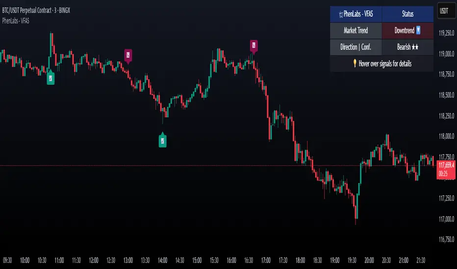
● Info Dashboard :
* Located at the top-right of the chart, providing a clean summary.
* Displays: "PhenLabs - VFAS" header, "Market Trend" (Uptrend/Downtrend/Range with color-coded status), and "Direction | Conf." (showing the last signal's direction and star confidence).
* Optional "💡 Hover over signals for details" reminder.
* Interpretation: A concise, real-time summary of the market's pulse and the most recent high-conviction event, helping traders stay informed at a glance.
📖 Usage Guidelines
Setting Categories
⚙️ Core Delta & Volume Engine
● Minimum Volume Lookback (Bars)
○ Default: 9
○ Range: Integer (e.g., 5-50)
○ Description: Defines the number of preceding bars used to calculate the average volume and delta. Bars with volume below this average won't be considered for high-volume signals. A shorter lookback is more reactive to recent changes, while a longer one provides a smoother average.
📈 Anomaly Detection Settings
Delta Z-Score Anomaly Threshold
○ Default: 2.5
○ Range: Float (e.g., 1.0-5.0+)
○ Description: The number of standard deviations from the mean that a bar's delta must exceed to be considered a significant anomaly. A higher threshold means fewer, but potentially stronger, signals. A lower threshold will generate more signals, which might include less significant events. Experiment to find the optimal balance for your trading style.
🔬 Context Filters
Enable Trend Filter
○ Default: False
○ Range: Boolean (True/False)
○ Description: When enabled, signals will only be generated if they align with the current market trend as determined by the EMAs (e.g., only bullish signals in an uptrend, bearish in a downtrend). This helps to filter out counter-trend noise.
● Trend EMA Fast
○ Default: 50
○ Range: Integer (e.g., 10-100)
○ Description: The period for the faster Exponential Moving Average used in the trend filter. In combination with the slow EMA, it defines the trend direction.
● Trend EMA Slow
○ Default: 200
○ Range: Integer (e.g., 100-400)
○ Description: The period for the slower Exponential Moving Average used in the trend filter. The relationship between the fast and slow EMA determines if the market is in an uptrend (fast > slow) or downtrend (fast < slow).
🎨 Visual & UI Settings
● Show Info Dashboard
○ Default: True
○ Range: Boolean (True/False)
○ Description: Toggles the visibility of the dashboard on the chart, which provides a summary of market trend and the last detected signal.
● Show Dashboard Tooltip
○ Default: True
○ Range: Boolean (True/False)
○ Description: Toggles a reminder message in the dashboard to hover over signal labels for more detailed information.
● Show Delta Anomaly Bar Colors
○ Default: True
○ Range: Boolean (True/False)
○ Description: Enables or disables the coloring of bars based on their delta direction and whether they represent a significant anomaly.
● Show Signal Labels
○ Default: True
○ Range: Boolean (True/False)
○ Description: Controls the visibility of the “📈” or “📉” labels that appear on the chart when a delta anomaly signal is generated.
🔔 Alert Settings
Alert on Delta Anomaly
○ Default: True
○ Range: Boolean (True/False)
○ Description: When enabled, this setting allows you to set up alerts in TradingView that will trigger whenever a new bullish or bearish delta anomaly is detected.
✅ Best Use Cases
Early Trend Reversal / Continuation Detection: Identify strong surges of buying/selling pressure at key support/resistance levels that could indicate a reversal or the continuation of a strong move.
● Confirmation of Breakouts: Use high-confidence delta anomalies to confirm the validity of price breakouts, indicating strong conviction behind the move.
● Entry and Exit Points: Pinpoint precise entry opportunities when anomalies align with your trading strategy, or identify potential exhaustion signals for exiting trades.
● Scalping and Day Trading: The indicator’s sensitivity to intraday buying/selling imbalances makes it highly effective for short-term trading strategies.
● Market Sentiment Analysis: Gain a real-time understanding of underlying market sentiment by observing the prevalence and strength of bullish vs. bearish anomalies.
⚠️ Limitations
Estimated Delta: The script uses a simplified method to estimate delta based on bar close relative to its range, not actual order book or footprint data. While effective, it’s an approximation.
● Sensitivity to Z-Score Threshold: The effectiveness heavily relies on the `Delta Z-Score Anomaly Threshold`. Too low, and you’ll get many false positives; too high, and you might miss valid signals.
● Confirmation Criteria: The 4-star confidence level’s “confirmation” relies on specific subsequent bar conditions and previous confirmed signals, which might be too strict or specific for all contexts.
● Requires Context: While powerful, VFAS is best used in conjunction with other technical analysis tools and price action to form a comprehensive trading strategy. It is not a standalone “buy/sell” signal.
💡 What Makes This Unique
Statistical Rigor: The application of Z-score analysis to bar delta provides an objective, statistically-driven way to identify true anomalies, moving beyond arbitrary thresholds.
● Multi-Factor Confidence Scoring: The unique 1-4 star confidence system integrates multiple market dynamics (volume, trend alignment, specific follow-through) into a single, easy-to-interpret rating.
● User-Friendly Design: From the intuitive dashboard to the detailed signal tooltips, the indicator prioritizes clear and accessible information for traders of all experience levels.
🔬 How It Works
1. Bar Delta Calculation:
● The script first estimates the “buy volume” and “sell volume” for each bar. This is done by assuming that volume proportional to the distance from the low to the close represents buying, and volume proportional to the distance from the high to the close represents selling.
● How this contributes: This provides a proxy for the net buying or selling pressure (delta) within that specific price bar, even without access to actual footprint data.
2. Volume & Delta Z-Score Analysis:
● The average volume over a user-defined lookback period is calculated. Bars with volume less than twice this average are generally considered of lower interest.
● The Z-score for the calculated bar delta is computed. The Z-score measures how many standard deviations the current bar’s delta is from its average delta over the `Minimum Volume Lookback` period.
● How this contributes: A high positive Z-score indicates a bullish delta anomaly (significantly more buying than usual), while a high negative Z-score indicates a bearish delta anomaly (significantly more selling than usual). This identifies statistically unusual levels of pressure.
3. Trend Filtering (Optional):
● Two Exponential Moving Averages (Fast and Slow EMA) are used to determine the prevailing market trend. An uptrend is identified when the Fast EMA is above the Slow EMA, and a downtrend when the Fast EMA is below the Slow EMA.
● How this contributes: If enabled, the indicator will only display bullish delta anomalies during an uptrend and bearish delta anomalies during a downtrend, helping to confirm signals within the broader market context and avoid counter-trend signals.
4. Signal Generation & Confidence Scoring:
● When a delta Z-score exceeds the user-defined anomaly threshold, a signal is generated.
● This signal is then passed through a multi-factor confidence algorithm (`f_calculateConfidence`). It awards stars based on: high volume presence, alignment with the overall trend (if enabled), and a fourth star for very strong Z-scores (above 3.0) combined with specific follow-through candle patterns after a cooling-off period from a previous confirmed signal.
● How this contributes: Provides a qualitative rating (1-4 stars) for each anomaly, allowing traders to quickly assess the potential significance and reliability of the signal.
💡 Note:
The PhenLabs Volume Footprint Anomaly Scanner is a powerful analytical tool, but it’s crucial to understand that no indicator guarantees profit. Always backtest and forward-test the indicator settings on your chosen assets and timeframes. Consider integrating VFAS with your existing trading strategy, using its signals as confirmation for entries, exits, or trend bias. The Z-score threshold is highly customizable; lower values will yield more signals (including potential noise), while higher values will provide fewer but potentially higher-conviction signals. Adjust this parameter based on market volatility and your risk tolerance. Remember to combine statistical insights from VFAS with price action, support/resistance levels, and your overall market outlook for optimal results.
Cari skrip untuk "Exponential"
BACAP PRICE STRUCTURE 21 EMA TREND21dma-STRUCTURE
Overview
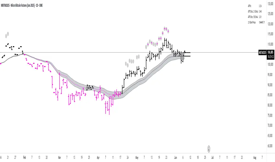
The 21dma-STRUCTURE indicator is a sophisticated overlay indicator that visualizes price action relative to a triple 21-period exponential moving average structure. Originally developed by BalarezoCapital and enhanced by PrimeTrading, this indicator provides clear visual cues for trend direction and momentum through dynamic bar coloring and EMA structure analysis.
Key Features
Triple EMA Structure
- 21 EMA High: Tracks the exponential moving average of high prices
- 21 EMA Close: Tracks the exponential moving average of closing prices
- 21 EMA Low: Tracks the exponential moving average of low prices
- Dynamic Cloud: Gray fill between high and low EMAs for visual structure reference
Smart Bar Coloring System
- Blue Bars: Price closes above all three EMAs (strong bullish momentum)
- Pink Bars: Daily high falls below the lowest EMA (strong bearish signal)
- Gray Bars: Neutral conditions or transitional phases
- Color Memory: Maintains previous color until new condition is met
Dynamic Center Line
- Trend-Following Color: Green when all EMAs are rising, red when all are falling
- Color Persistence: Maintains trend color during sideways movement
- Visual Clarity: Thicker center line for easy trend identification
Customizable Visual Elements
- Adjustable line thickness for all EMA plots
- Customizable colors for bullish and bearish conditions
- Configurable trend colors for uptrend and downtrend phases
- Optional bar color changes with toggle control
How to Use
Trend Identification
- Rising Green Center Line: All EMAs trending upward (bullish structure)
- Falling Red Center Line: All EMAs trending downward (bearish structure)
- Flat Center Line: Maintains last trend color during consolidation
Momentum Analysis
- Blue Bars: Strong bullish momentum with price above entire EMA structure
- Pink Bars: Strong bearish momentum with high below lowest EMA
- Gray Bars: Neutral or transitional momentum phases
Entry and Exit Signals
- Bullish Setup: Look for blue bars during green center line periods
- Bearish Setup: Look for pink bars during red center line periods
- Exit Consideration: Watch for color changes as potential momentum shifts
Structure Trading
- Support/Resistance: Use EMA cloud as dynamic support and resistance zones
- Breakout Confirmation: Bar color changes can confirm structure breakouts
- Trend Continuation: Color persistence suggests ongoing momentum
Settings
Visual Customization
- Change Bar Color: Toggle to enable/disable bar coloring
- Line Size: Adjust thickness of EMA lines (default: 3)
- Bullish Candle Color: Customize blue bar color
- Bearish Candle Color: Customize pink bar color
Trend Colors
- Uptrend Color: Color for rising EMA center line (default: green)
- Downtrend Color: Color for falling EMA center line (default: red)
- Cloud Color: Fill color between high and low EMAs (default: gray)
Advanced Features
Modified Bar Logic
Unlike traditional EMA systems, this indicator uses refined conditions:
- Bullish signals require close above ALL three EMAs
- Bearish signals require high below the LOWEST EMA
- Enhanced precision reduces false signals compared to single EMA systems
Trend Memory System
- Intelligent color persistence during sideways movement
- Reduces noise from minor EMA fluctuations
- Maintains trend context during consolidation periods
Performance Optimization
- Efficient calculation methods for real-time performance
- Clean visual design that doesn't clutter charts
- Compatible with all timeframes and instruments
Best Practices
Multi-Timeframe Analysis
- Use higher timeframes to identify overall trend direction
- Apply on multiple timeframes for confluence
- Combine with weekly/monthly charts for position trading
Risk Management
- Use bar color changes as early warning signals
- Consider position sizing based on EMA structure strength
- Set stops relative to EMA support/resistance levels
Combination Strategies
- Pair with volume indicators for confirmation
- Use alongside RSI or MACD for momentum confirmation
- Combine with key support/resistance levels
Market Context
- More effective in trending markets than choppy conditions
- Consider overall market environment and sector strength
- Adjust expectations during high volatility periods
Technical Specifications
- Based on 21-period exponential moving averages
- Uses Pine Script v6 for optimal performance
- Overlay indicator that works with any chart type
- Maximum 500 lines for clean performance
Ideal Applications
- Swing trading on daily charts
- Position trading on weekly charts
- Intraday momentum trading (adjust timeframe accordingly)
- Trend following strategies
- Structure-based trading approaches
Disclaimer
This indicator is for educational and informational purposes only. It should not be used as the sole basis for trading decisions. Always combine with other forms of analysis, proper risk management, and consider your individual trading plan and risk tolerance.
Compatible with Pine Script v6 | Works on all timeframes | Optimized for trending markets
Kernel Weighted DMI | QuantEdgeB📊 Introducing Kernel Weighted DMI (K-DMI) by QuantEdgeB
🛠️ Overview
K-DMI is a next-gen momentum indicator that combines the traditional Directional Movement Index (DMI) with advanced kernel smoothing techniques to produce a highly adaptive, noise-resistant trend signal.
Unlike standard DMI that can be overly reactive or choppy in consolidation phases, K-DMI applies kernel-weighted filtering (Linear, Exponential, or Gaussian) to stabilize directional movement readings and extract a more reliable momentum signal.
✨ Key Features
🔹 Kernel Smoothing Engine
Smooths DMI using your choice of kernel (Linear, Exponential, Gaussian) for flexible noise reduction and clarity.
🔹 Dynamic Trend Signal
Generates real-time long/short trend bias based on signal crossing upper or lower thresholds (defaults: ±1).
🔹 Visual Encoding
Includes directional gradient fills, candle coloring, and momentum-based overlays for instant signal comprehension.
🔹 Multi-Mode Plotting
Optional moving average overlays visualize structure and compression/expansion within price action.
📐 How It Works
1️⃣ Directional Movement Index (DMI)
Calculates the traditional +DI and -DI differential to derive directional bias.
2️⃣ Kernel-Based Smoothing
Applies a custom-weighted average across historical DMI values using one of three smoothing methods:
• Linear → Simple tapering weights
• Exponential → Decay curve for recent emphasis
• Gaussian → Bell-shaped weight for centered precision
3️⃣ Signal Generation
• ✅ Long → Signal > Long Threshold (default: +1)
• ❌ Short → Signal < Short Threshold (default: -1)
Additional overlays signal potential compression zones or trend resumption using gradient and line fills.
⚙️ Custom Settings
• DMI Length: Default = 7
• Kernel Type: Options → Linear, Exponential, Gaussian (Def:Linear)
• Kernel Length: Default = 25
• Long Threshold: Default = 1
• Short Threshold: Default = -1
• Color Mode: Strategy, Solar, Warm, Cool, Classic, Magic
• Show Labels: Optional entry signal labels (Long/Short)
• Enable Extra Plots: Toggle MA overlays and dynamic bands
👥 Who Is It For?
✅ Trend Traders → Identify sustained directional bias with smoother signal lines
✅ Quant Analysts → Leverage advanced smoothing models to enhance data clarity
✅ Discretionary Swing Traders → Visualize clean breakouts or fades within choppy zones
✅ MA Compression Traders → Use overlay MAs to detect expansion opportunities
📌 Conclusion
Kernel Weighted DMI is the evolution of classic momentum tracking—merging traditional DMI logic with adaptable kernel filters. It provides a refined lens for trend detection, while optional visual overlays support price structure analysis.
🔹 Key Takeaways:
1️⃣ Smoothed and stabilized DMI for reliable trend signal generation
2️⃣ Optional Gaussian/exponential weighting for adaptive responsiveness
3️⃣ Custom gradient fills, dynamic MAs, and candle coloring to support visual clarity
📌 Disclaimer: Past performance is not indicative of future results. No trading strategy can guarantee success in financial markets.
📌 Strategic Advice: Always backtest, optimize, and align parameters with your trading objectives and risk tolerance before live trading.

real_time_candlesIntroduction
The Real-Time Candles Library provides comprehensive tools for creating, manipulating, and visualizing custom timeframe candles in Pine Script. Unlike standard indicators that only update at bar close, this library enables real-time visualization of price action and indicators within the current bar, offering traders unprecedented insight into market dynamics as they unfold.
This library addresses a fundamental limitation in traditional technical analysis: the inability to see how indicators evolve between bar closes. By implementing sophisticated real-time data processing techniques, traders can now observe indicator movements, divergences, and trend changes as they develop, potentially identifying trading opportunities much earlier than with conventional approaches.
Key Features
The library supports two primary candle generation approaches:
Chart-Time Candles: Generate real-time OHLC data for any variable (like RSI, MACD, etc.) while maintaining synchronization with chart bars.
Custom Timeframe (CTF) Candles: Create candles with custom time intervals or tick counts completely independent of the chart's native timeframe.
Both approaches support traditional candlestick and Heikin-Ashi visualization styles, with options for moving average overlays to smooth the data.
Configuration Requirements
For optimal performance with this library:
Set max_bars_back = 5000 in your script settings
When using CTF drawing functions, set max_lines_count = 500, max_boxes_count = 500, and max_labels_count = 500
These settings ensure that you will be able to draw correctly and will avoid any runtime errors.
Usage Examples
Basic Chart-Time Candle Visualization
// Create real-time candles for RSI
float rsi = ta.rsi(close, 14)
Candle rsi_candle = candle_series(rsi, CandleType.candlestick)
// Plot the candles using Pine's built-in function
plotcandle(rsi_candle.Open, rsi_candle.High, rsi_candle.Low, rsi_candle.Close,
"RSI Candles", rsi_candle.candle_color, rsi_candle.candle_color)
Multiple Access Patterns
The library provides three ways to access candle data, accommodating different programming styles:
// 1. Array-based access for collection operations
Candle candles = candle_array(source)
// 2. Object-oriented access for single entity manipulation
Candle candle = candle_series(source)
float value = candle.source(Source.HLC3)
// 3. Tuple-based access for functional programming styles
= candle_tuple(source)
Custom Timeframe Examples
// Create 20-second candles with EMA overlay
plot_ctf_candles(
source = close,
candle_type = CandleType.candlestick,
sample_type = SampleType.Time,
number_of_seconds = 20,
timezone = -5,
tied_open = true,
ema_period = 9,
enable_ema = true
)
// Create tick-based candles (new candle every 15 ticks)
plot_ctf_tick_candles(
source = close,
candle_type = CandleType.heikin_ashi,
number_of_ticks = 15,
timezone = -5,
tied_open = true
)
Advanced Usage with Custom Visualization
// Get custom timeframe candles without automatic plotting
CandleCTF my_candles = ctf_candles_array(
source = close,
candle_type = CandleType.candlestick,
sample_type = SampleType.Time,
number_of_seconds = 30
)
// Apply custom logic to the candles
float ema_values = my_candles.ctf_ema(14)
// Draw candles and EMA using time-based coordinates
my_candles.draw_ctf_candles_time()
ema_values.draw_ctf_line_time(line_color = #FF6D00)
Library Components
Data Types
Candle: Structure representing chart-time candles with OHLC, polarity, and visualization properties
CandleCTF: Extended candle structure with additional time metadata for custom timeframes
TickData: Structure for individual price updates with time deltas
Enumerations
CandleType: Specifies visualization style (candlestick or Heikin-Ashi)
Source: Defines price components for calculations (Open, High, Low, Close, HL2, etc.)
SampleType: Sets sampling method (Time-based or Tick-based)
Core Functions
get_tick(): Captures current price as a tick data point
candle_array(): Creates an array of candles from price updates
candle_series(): Provides a single candle based on latest data
candle_tuple(): Returns OHLC values as a tuple
ctf_candles_array(): Creates custom timeframe candles without rendering
Visualization Functions
source(): Extracts specific price components from candles
candle_ctf_to_float(): Converts candle data to float arrays
ctf_ema(): Calculates exponential moving averages for candle arrays
draw_ctf_candles_time(): Renders candles using time coordinates
draw_ctf_candles_index(): Renders candles using bar index coordinates
draw_ctf_line_time(): Renders lines using time coordinates
draw_ctf_line_index(): Renders lines using bar index coordinates
Technical Implementation Notes
This library leverages Pine Script's varip variables for state management, creating a sophisticated real-time data processing system. The implementation includes:
Efficient tick capturing: Samples price at every execution, maintaining temporal tracking with time deltas
Smart state management: Uses a hybrid approach with mutable updates at index 0 and historical preservation at index 1+
Temporal synchronization: Manages two time domains (chart time and custom timeframe)
The tooltip implementation provides crucial temporal context for custom timeframe visualizations, allowing users to understand exactly when each candle formed regardless of chart timeframe.
Limitations
Custom timeframe candles cannot be backtested due to Pine Script's limitations with historical tick data
Real-time visualization is only available during live chart updates
Maximum history is constrained by Pine Script's array size limits
Applications
Indicator visualization: See how RSI, MACD, or other indicators evolve in real-time
Volume analysis: Create custom volume profiles independent of chart timeframe
Scalping strategies: Identify short-term patterns with precisely defined time windows
Volatility measurement: Track price movement characteristics within bars
Custom signal generation: Create entry/exit signals based on custom timeframe patterns
Conclusion
The Real-Time Candles Library bridges the gap between traditional technical analysis (based on discrete OHLC bars) and the continuous nature of market movement. By making indicators more responsive to real-time price action, it gives traders a significant edge in timing and decision-making, particularly in fast-moving markets where waiting for bar close could mean missing important opportunities.
Whether you're building custom indicators, researching price patterns, or developing trading strategies, this library provides the foundation for sophisticated real-time analysis in Pine Script.
Implementation Details & Advanced Guide
Core Implementation Concepts
The Real-Time Candles Library implements a sophisticated event-driven architecture within Pine Script's constraints. At its heart, the library creates what's essentially a reactive programming framework handling continuous data streams.
Tick Processing System
The foundation of the library is the get_tick() function, which captures price updates as they occur:
export get_tick(series float source = close, series float na_replace = na)=>
varip float price = na
varip int series_index = -1
varip int old_time = 0
varip int new_time = na
varip float time_delta = 0
// ...
This function:
Samples the current price
Calculates time elapsed since last update
Maintains a sequential index to track updates
The resulting TickData structure serves as the fundamental building block for all candle generation.
State Management Architecture
The library employs a sophisticated state management system using varip variables, which persist across executions within the same bar. This creates a hybrid programming paradigm that's different from standard Pine Script's bar-by-bar model.
For chart-time candles, the core state transition logic is:
// Real-time update of current candle
candle_data := Candle.new(Open, High, Low, Close, polarity, series_index, candle_color)
candles.set(0, candle_data)
// When a new bar starts, preserve the previous candle
if clear_state
candles.insert(1, candle_data)
price.clear()
// Reset state for new candle
Open := Close
price.push(Open)
series_index += 1
This pattern of updating index 0 in real-time while inserting completed candles at index 1 creates an elegant solution for maintaining both current state and historical data.
Custom Timeframe Implementation
The custom timeframe system manages its own time boundaries independent of chart bars:
bool clear_state = switch settings.sample_type
SampleType.Ticks => cumulative_series_idx >= settings.number_of_ticks
SampleType.Time => cumulative_time_delta >= settings.number_of_seconds
This dual-clock system synchronizes two time domains:
Pine's execution clock (bar-by-bar processing)
The custom timeframe clock (tick or time-based)
The library carefully handles temporal discontinuities, ensuring candle formation remains accurate despite irregular tick arrival or market gaps.
Advanced Usage Techniques
1. Creating Custom Indicators with Real-Time Candles
To develop indicators that process real-time data within the current bar:
// Get real-time candles for your data
Candle rsi_candles = candle_array(ta.rsi(close, 14))
// Calculate indicator values based on candle properties
float signal = ta.ema(rsi_candles.first().source(Source.Close), 9)
// Detect patterns that occur within the bar
bool divergence = close > close and rsi_candles.first().Close < rsi_candles.get(1).Close
2. Working with Custom Timeframes and Plotting
For maximum flexibility when visualizing custom timeframe data:
// Create custom timeframe candles
CandleCTF volume_candles = ctf_candles_array(
source = volume,
candle_type = CandleType.candlestick,
sample_type = SampleType.Time,
number_of_seconds = 60
)
// Convert specific candle properties to float arrays
float volume_closes = volume_candles.candle_ctf_to_float(Source.Close)
// Calculate derived values
float volume_ema = volume_candles.ctf_ema(14)
// Create custom visualization
volume_candles.draw_ctf_candles_time()
volume_ema.draw_ctf_line_time(line_color = color.orange)
3. Creating Hybrid Timeframe Analysis
One powerful application is comparing indicators across multiple timeframes:
// Standard chart timeframe RSI
float chart_rsi = ta.rsi(close, 14)
// Custom 5-second timeframe RSI
CandleCTF ctf_candles = ctf_candles_array(
source = close,
candle_type = CandleType.candlestick,
sample_type = SampleType.Time,
number_of_seconds = 5
)
float fast_rsi_array = ctf_candles.candle_ctf_to_float(Source.Close)
float fast_rsi = fast_rsi_array.first()
// Generate signals based on divergence between timeframes
bool entry_signal = chart_rsi < 30 and fast_rsi > fast_rsi_array.get(1)
Final Notes
This library represents an advanced implementation of real-time data processing within Pine Script's constraints. By creating a reactive programming framework for handling continuous data streams, it enables sophisticated analysis typically only available in dedicated trading platforms.
The design principles employed—including state management, temporal processing, and object-oriented architecture—can serve as patterns for other advanced Pine Script development beyond this specific application.
------------------------
Library "real_time_candles"
A comprehensive library for creating real-time candles with customizable timeframes and sampling methods.
Supports both chart-time and custom-time candles with options for candlestick and Heikin-Ashi visualization.
Allows for tick-based or time-based sampling with moving average overlay capabilities.
get_tick(source, na_replace)
Captures the current price as a tick data point
Parameters:
source (float) : Optional - Price source to sample (defaults to close)
na_replace (float) : Optional - Value to use when source is na
Returns: TickData structure containing price, time since last update, and sequential index
candle_array(source, candle_type, sync_start, bullish_color, bearish_color)
Creates an array of candles based on price updates
Parameters:
source (float) : Optional - Price source to sample (defaults to close)
candle_type (simple CandleType) : Optional - Type of candle chart to create (candlestick or Heikin-Ashi)
sync_start (simple bool) : Optional - Whether to synchronize with the start of a new bar
bullish_color (color) : Optional - Color for bullish candles
bearish_color (color) : Optional - Color for bearish candles
Returns: Array of Candle objects ordered with most recent at index 0
candle_series(source, candle_type, wait_for_sync, bullish_color, bearish_color)
Provides a single candle based on the latest price data
Parameters:
source (float) : Optional - Price source to sample (defaults to close)
candle_type (simple CandleType) : Optional - Type of candle chart to create (candlestick or Heikin-Ashi)
wait_for_sync (simple bool) : Optional - Whether to wait for a new bar before starting
bullish_color (color) : Optional - Color for bullish candles
bearish_color (color) : Optional - Color for bearish candles
Returns: A single Candle object representing the current state
candle_tuple(source, candle_type, wait_for_sync, bullish_color, bearish_color)
Provides candle data as a tuple of OHLC values
Parameters:
source (float) : Optional - Price source to sample (defaults to close)
candle_type (simple CandleType) : Optional - Type of candle chart to create (candlestick or Heikin-Ashi)
wait_for_sync (simple bool) : Optional - Whether to wait for a new bar before starting
bullish_color (color) : Optional - Color for bullish candles
bearish_color (color) : Optional - Color for bearish candles
Returns: Tuple representing current candle values
method source(self, source, na_replace)
Extracts a specific price component from a Candle
Namespace types: Candle
Parameters:
self (Candle)
source (series Source) : Type of price data to extract (Open, High, Low, Close, or composite values)
na_replace (float) : Optional - Value to use when source value is na
Returns: The requested price value from the candle
method source(self, source)
Extracts a specific price component from a CandleCTF
Namespace types: CandleCTF
Parameters:
self (CandleCTF)
source (simple Source) : Type of price data to extract (Open, High, Low, Close, or composite values)
Returns: The requested price value from the candle as a varip
method candle_ctf_to_float(self, source)
Converts a specific price component from each CandleCTF to a float array
Namespace types: array
Parameters:
self (array)
source (simple Source) : Optional - Type of price data to extract (defaults to Close)
Returns: Array of float values extracted from the candles, ordered with most recent at index 0
method ctf_ema(self, ema_period)
Calculates an Exponential Moving Average for a CandleCTF array
Namespace types: array
Parameters:
self (array)
ema_period (simple float) : Period for the EMA calculation
Returns: Array of float values representing the EMA of the candle data, ordered with most recent at index 0
method draw_ctf_candles_time(self, sample_type, number_of_ticks, number_of_seconds, timezone)
Renders custom timeframe candles using bar time coordinates
Namespace types: array
Parameters:
self (array)
sample_type (simple SampleType) : Optional - Method for sampling data (Time or Ticks), used for tooltips
number_of_ticks (simple int) : Optional - Number of ticks per candle (used when sample_type is Ticks), used for tooltips
number_of_seconds (simple float) : Optional - Time duration per candle in seconds (used when sample_type is Time), used for tooltips
timezone (simple int) : Optional - Timezone offset from UTC (-12 to +12), used for tooltips
Returns: void - Renders candles on the chart using time-based x-coordinates
method draw_ctf_candles_index(self, sample_type, number_of_ticks, number_of_seconds, timezone)
Renders custom timeframe candles using bar index coordinates
Namespace types: array
Parameters:
self (array)
sample_type (simple SampleType) : Optional - Method for sampling data (Time or Ticks), used for tooltips
number_of_ticks (simple int) : Optional - Number of ticks per candle (used when sample_type is Ticks), used for tooltips
number_of_seconds (simple float) : Optional - Time duration per candle in seconds (used when sample_type is Time), used for tooltips
timezone (simple int) : Optional - Timezone offset from UTC (-12 to +12), used for tooltips
Returns: void - Renders candles on the chart using index-based x-coordinates
method draw_ctf_line_time(self, source, line_size, line_color)
Renders a line representing a price component from the candles using time coordinates
Namespace types: array
Parameters:
self (array)
source (simple Source) : Optional - Type of price data to extract (defaults to Close)
line_size (simple int) : Optional - Width of the line
line_color (simple color) : Optional - Color of the line
Returns: void - Renders a connected line on the chart using time-based x-coordinates
method draw_ctf_line_time(self, line_size, line_color)
Renders a line from a varip float array using time coordinates
Namespace types: array
Parameters:
self (array)
line_size (simple int) : Optional - Width of the line, defaults to 2
line_color (simple color) : Optional - Color of the line
Returns: void - Renders a connected line on the chart using time-based x-coordinates
method draw_ctf_line_index(self, source, line_size, line_color)
Renders a line representing a price component from the candles using index coordinates
Namespace types: array
Parameters:
self (array)
source (simple Source) : Optional - Type of price data to extract (defaults to Close)
line_size (simple int) : Optional - Width of the line
line_color (simple color) : Optional - Color of the line
Returns: void - Renders a connected line on the chart using index-based x-coordinates
method draw_ctf_line_index(self, line_size, line_color)
Renders a line from a varip float array using index coordinates
Namespace types: array
Parameters:
self (array)
line_size (simple int) : Optional - Width of the line, defaults to 2
line_color (simple color) : Optional - Color of the line
Returns: void - Renders a connected line on the chart using index-based x-coordinates
plot_ctf_tick_candles(source, candle_type, number_of_ticks, timezone, tied_open, ema_period, bullish_color, bearish_color, line_width, ema_color, use_time_indexing)
Plots tick-based candles with moving average
Parameters:
source (float) : Input price source to sample
candle_type (simple CandleType) : Type of candle chart to display
number_of_ticks (simple int) : Number of ticks per candle
timezone (simple int) : Timezone offset from UTC (-12 to +12)
tied_open (simple bool) : Whether to tie open price to close of previous candle
ema_period (simple float) : Period for the exponential moving average
bullish_color (color) : Optional - Color for bullish candles
bearish_color (color) : Optional - Color for bearish candles
line_width (simple int) : Optional - Width of the moving average line, defaults to 2
ema_color (color) : Optional - Color of the moving average line
use_time_indexing (simple bool) : Optional - When true the function will plot with xloc.time, when false it will plot using xloc.bar_index
Returns: void - Creates visual candle chart with EMA overlay
plot_ctf_tick_candles(source, candle_type, number_of_ticks, timezone, tied_open, bullish_color, bearish_color, use_time_indexing)
Plots tick-based candles without moving average
Parameters:
source (float) : Input price source to sample
candle_type (simple CandleType) : Type of candle chart to display
number_of_ticks (simple int) : Number of ticks per candle
timezone (simple int) : Timezone offset from UTC (-12 to +12)
tied_open (simple bool) : Whether to tie open price to close of previous candle
bullish_color (color) : Optional - Color for bullish candles
bearish_color (color) : Optional - Color for bearish candles
use_time_indexing (simple bool) : Optional - When true the function will plot with xloc.time, when false it will plot using xloc.bar_index
Returns: void - Creates visual candle chart without moving average
plot_ctf_time_candles(source, candle_type, number_of_seconds, timezone, tied_open, ema_period, bullish_color, bearish_color, line_width, ema_color, use_time_indexing)
Plots time-based candles with moving average
Parameters:
source (float) : Input price source to sample
candle_type (simple CandleType) : Type of candle chart to display
number_of_seconds (simple float) : Time duration per candle in seconds
timezone (simple int) : Timezone offset from UTC (-12 to +12)
tied_open (simple bool) : Whether to tie open price to close of previous candle
ema_period (simple float) : Period for the exponential moving average
bullish_color (color) : Optional - Color for bullish candles
bearish_color (color) : Optional - Color for bearish candles
line_width (simple int) : Optional - Width of the moving average line, defaults to 2
ema_color (color) : Optional - Color of the moving average line
use_time_indexing (simple bool) : Optional - When true the function will plot with xloc.time, when false it will plot using xloc.bar_index
Returns: void - Creates visual candle chart with EMA overlay
plot_ctf_time_candles(source, candle_type, number_of_seconds, timezone, tied_open, bullish_color, bearish_color, use_time_indexing)
Plots time-based candles without moving average
Parameters:
source (float) : Input price source to sample
candle_type (simple CandleType) : Type of candle chart to display
number_of_seconds (simple float) : Time duration per candle in seconds
timezone (simple int) : Timezone offset from UTC (-12 to +12)
tied_open (simple bool) : Whether to tie open price to close of previous candle
bullish_color (color) : Optional - Color for bullish candles
bearish_color (color) : Optional - Color for bearish candles
use_time_indexing (simple bool) : Optional - When true the function will plot with xloc.time, when false it will plot using xloc.bar_index
Returns: void - Creates visual candle chart without moving average
plot_ctf_candles(source, candle_type, sample_type, number_of_ticks, number_of_seconds, timezone, tied_open, ema_period, bullish_color, bearish_color, enable_ema, line_width, ema_color, use_time_indexing)
Unified function for plotting candles with comprehensive options
Parameters:
source (float) : Input price source to sample
candle_type (simple CandleType) : Optional - Type of candle chart to display
sample_type (simple SampleType) : Optional - Method for sampling data (Time or Ticks)
number_of_ticks (simple int) : Optional - Number of ticks per candle (used when sample_type is Ticks)
number_of_seconds (simple float) : Optional - Time duration per candle in seconds (used when sample_type is Time)
timezone (simple int) : Optional - Timezone offset from UTC (-12 to +12)
tied_open (simple bool) : Optional - Whether to tie open price to close of previous candle
ema_period (simple float) : Optional - Period for the exponential moving average
bullish_color (color) : Optional - Color for bullish candles
bearish_color (color) : Optional - Color for bearish candles
enable_ema (bool) : Optional - Whether to display the EMA overlay
line_width (simple int) : Optional - Width of the moving average line, defaults to 2
ema_color (color) : Optional - Color of the moving average line
use_time_indexing (simple bool) : Optional - When true the function will plot with xloc.time, when false it will plot using xloc.bar_index
Returns: void - Creates visual candle chart with optional EMA overlay
ctf_candles_array(source, candle_type, sample_type, number_of_ticks, number_of_seconds, tied_open, bullish_color, bearish_color)
Creates an array of custom timeframe candles without rendering them
Parameters:
source (float) : Input price source to sample
candle_type (simple CandleType) : Type of candle chart to create (candlestick or Heikin-Ashi)
sample_type (simple SampleType) : Method for sampling data (Time or Ticks)
number_of_ticks (simple int) : Optional - Number of ticks per candle (used when sample_type is Ticks)
number_of_seconds (simple float) : Optional - Time duration per candle in seconds (used when sample_type is Time)
tied_open (simple bool) : Optional - Whether to tie open price to close of previous candle
bullish_color (color) : Optional - Color for bullish candles
bearish_color (color) : Optional - Color for bearish candles
Returns: Array of CandleCTF objects ordered with most recent at index 0
Candle
Structure representing a complete candle with price data and display properties
Fields:
Open (series float) : Opening price of the candle
High (series float) : Highest price of the candle
Low (series float) : Lowest price of the candle
Close (series float) : Closing price of the candle
polarity (series bool) : Boolean indicating if candle is bullish (true) or bearish (false)
series_index (series int) : Sequential index identifying the candle in the series
candle_color (series color) : Color to use when rendering the candle
ready (series bool) : Boolean indicating if candle data is valid and ready for use
TickData
Structure for storing individual price updates
Fields:
price (series float) : The price value at this tick
time_delta (series float) : Time elapsed since the previous tick in milliseconds
series_index (series int) : Sequential index identifying this tick
CandleCTF
Structure representing a custom timeframe candle with additional time metadata
Fields:
Open (series float) : Opening price of the candle
High (series float) : Highest price of the candle
Low (series float) : Lowest price of the candle
Close (series float) : Closing price of the candle
polarity (series bool) : Boolean indicating if candle is bullish (true) or bearish (false)
series_index (series int) : Sequential index identifying the candle in the series
open_time (series int) : Timestamp marking when the candle was opened (in Unix time)
time_delta (series float) : Duration of the candle in milliseconds
candle_color (series color) : Color to use when rendering the candle

Adaptive DEMA Momentum Oscillator (ADMO)Overview:
The Adaptive DEMA Momentum Oscillator (ADMO) is an open-source technical analysis tool developed to measure market momentum using a Double Exponential Moving Average (DEMA) and adaptive standard deviation. By dynamically combining price deviation from the moving average with normalized standard deviation, ADMO provides traders with a powerful way to interpret market conditions.
Key Features:
Double Exponential Moving Average (DEMA):
The core calculation of the indicator is based on DEMA, which is known for being more responsive to price changes compared to traditional moving averages. This makes the ADMO capable of capturing trend momentum effectively.
Standard Deviation Integration:
A normalized standard deviation is used to adaptively weight the oscillator. This makes the indicator more sensitive to market volatility, enhancing responsiveness during high volatility and reducing sensitivity during calmer periods.
Oscillator Representation:
The final oscillator value is derived from the combination of the DEMA-based Z-score and the normalized standard deviation. This final value is visualized as a color-coded histogram, reflecting bullish or bearish momentum.
Color-Coded Histogram:
Bullish Momentum: Values above zero are colored using a customizable bullish color (default: light green).
Bearish Momentum: Values below zero are colored using a customizable bearish color (default: red).
How It Works:
Inputs:
DEMA Length: Defines the period used for calculating the Double Exponential Moving Average. It can be adjusted from 1 to 200 to suit different trading styles.
Standard Deviation Length: Sets the lookback period for standard deviation calculations, which influences the responsiveness of the oscillator.
Standard Deviation Weight (StdDev Weight): Controls the weight given to the normalized standard deviation, allowing customization of the oscillator's sensitivity to volatility.
Calculation Steps:
Double Exponential Moving Average Calculation:
The DEMA is calculated using two exponential moving averages, which helps in reducing lag compared to a simple moving average.
Z-score Calculation:
The Z-score is derived by comparing the difference between the DEMA and its smoothed average (LSMA) to the standard deviation. This indicates how far the current value is from the mean in units of standard deviation.
Normalized Standard Deviation:
The standard deviation is normalized by subtracting the mean standard deviation and dividing by the standard deviation of the values. This helps to make the oscillator adaptive to recent changes in volatility.
Final Oscillator Value:
The final value is calculated by multiplying the Z-score with a factor based on the normalized standard deviation, resulting in a momentum indicator that adapts to different market conditions.
Visualization:
Histogram: The oscillator is plotted as a histogram, with color-coded bars showing the strength and direction of market momentum.
Positive (bullish) values are shown in green, indicating upward momentum.
Negative (bearish) values are shown in red, indicating downward momentum.
Zero Line: A zero line is plotted to provide a reference point, helping users quickly determine whether the current momentum is bullish or bearish.
Example Use Cases:
Momentum Identification:
ADMO helps identify the current market momentum by dynamically adapting to changes in market volatility. When the histogram is above zero and green, it indicates bullish conditions, whereas values below zero and red suggest bearish momentum.
Volatility-Adjusted Signals:
The normalized standard deviation weighting allows the ADMO to provide more reliable signals during different market conditions. This makes it particularly useful for traders who want to be responsive to market volatility while avoiding false signals.
Trend Confirmation and Divergence:
ADMO can be used to confirm the strength of a trend or identify potential divergences between price and momentum. This helps traders spot potential reversal points or continuation signals.
Summary:
The Adaptive DEMA Momentum Oscillator (ADMO) offers a unique approach by combining momentum analysis with adaptive standard deviation. The integration of DEMA makes it responsive to price changes, while the standard deviation adjustment helps it stay relevant in both high and low volatility environments. It's a versatile tool for traders who need an adaptive, momentum-based approach to technical analysis.
Feel free to explore the code and adapt it to your trading strategy. The open-source nature of this tool allows you to adjust the settings and visualize the output to fit your personal trading preferences.

Cinnamon_Bear Indicators MA LibraryLibrary "Cinnamon_BearIndicatorsMALibrary"
This is a personal Library of the NON built-in PineScript Moving Average function used to code indicators
ma_dema(source, length)
Double Exponential Moving Average (DEMA)
Parameters:
source (simple float)
length (simple int)
Returns: A double level of smoothing helps to follow price movements more closely while still reducing noise compared to a single EMA.
ma_dsma(source, length)
Double Smoothed Moving Average (DSMA)
Parameters:
source (simple float)
length (simple int)
Returns: A double level of smoothing helps to follow price movements more closely while still reducing noise compared to a single SMA.
ma_tema(source, length)
Triple Exponential Moving Average (TEMA)
Parameters:
source (simple float)
length (simple int)
Returns: A Triple level of smoothing helps to follow price movements even more closely compared to a DEMA.
ma_vwema(source, length)
Volume-Weighted Exponential Moving Average (VWEMA)
Parameters:
source (simple float)
length (simple int)
Returns: The VWEMA weights based on volume and recent price, giving more weight to periods with higher trading volumes.
ma_hma(source, length)
Hull Moving Average (HMA)
Parameters:
source (simple float)
length (simple int)
Returns: The HMA formula combines the properties of the weighted moving average (WMA) and the exponential moving average (EMA) to achieve a smoother and more responsive curve.
ma_ehma(source, length)
Enhanced Moving Average (EHMA)
Parameters:
source (simple float)
length (simple int)
Returns: The EHMA is calculated similarly to the Hull Moving Average (HMA) but uses a different weighting factor to further improve responsiveness.
ma_trix(source, length)
Triple Exponential Moving Average (TRIX)
Parameters:
source (simple float)
length (simple int)
Returns: The TRIX is an oscillator that shows the percentage change of a triple EMA. It is designed to filter out minor price movements and display only the most significant trends. The TRIX is a momentum indicator that can help identify trends and buy or sell signals.
ma_lsma(source, length)
Linear Weighted Moving Average (LSMA)
Parameters:
source (simple float)
length (simple int)
Returns: A moving average that gives more weight to recent prices. It is calculated using a formula that assigns linear weights to prices, with the highest weight given to the most recent price and the lowest weight given to the furthest price in the series.
ma_wcma(source, length)
Weighted Cumulative Moving Average (WCMA)
Parameters:
source (simple float)
length (simple int)
Returns: A moving average that gives more weight to recent prices. Compared to a LSMA, the WCMA the weights of data increase linearly with time, so the most recent data has a greater weight compared to older data. This means that the contribution of the most recent data to the moving average is more significant.
ma_vidya(source, length)
Variable Index Dynamic Average (VIDYA)
Parameters:
source (simple float)
length (simple int)
Returns: It is an adaptive moving average that adjusts its momentum based on market volatility using the formula of Chande Momentum Oscillator (CMO) .
ma_zlma(source, length)
Zero-Lag Moving Average (ZLMA)
Parameters:
source (simple float)
length (simple int)
Returns: Its aims to minimize the lag typically associated with MA, designed to react more quickly to price changes.
ma_gma(source, length, power)
Generalized Moving Average (GMA)
Parameters:
source (simple float)
length (simple int)
power (simple int)
Returns: It is a moving average that uses a power parameter to adjust the weight of historical data. This allows the GMA to adapt to various styles of MA.
ma_tma(source, length)
Triangular Moving Average (TMA)
Parameters:
source (simple float)
length (simple int)
Returns: MA more sensitive to changes in recent data compared to the SMA, providing a moving average that better adapts to short-term price changes.

Leading T3Hello Fellas,
Here, I applied a special technique of John F. Ehlers to make lagging indicators leading. The T3 itself is usually not realling the classic lagging indicator, so it is not really needed, but I still publish this indicator to demonstrate this technique of Ehlers applied on a simple indicator.
The indicator does not repaint.
In the following picture you can see a comparison of normal T3 (purple) compared to a 2-bar "leading" T3 (gradient):
The range of the gradient is:
Bottom Value: the lowest slope of the last 100 bars -> green
Top Value: the highest slope of the last 100 bars -> purple
Ehlers Special Technique
John Ehlers did develop methods to make lagging indicators leading or predictive. One of these methods is the Predictive Moving Average, which he introduced in his book “Rocket Science for Traders”. The concept is to take a difference of a lagging line from the original function to produce a leading function.
The idea is to extend this concept to moving averages. If you take a 7-bar Weighted Moving Average (WMA) of prices, that average lags the prices by 2 bars. If you take a 7-bar WMA of the first average, this second average is delayed another 2 bars. If you take the difference between the two averages and add that difference to the first average, the result should be a smoothed line of the original price function with no lag.
T3
To compute the T3 moving average, it involves a triple smoothing process using exponential moving averages. Here's how it works:
Calculate the first exponential moving average (EMA1) of the price data over a specific period 'n.'
Calculate the second exponential moving average (EMA2) of EMA1 using the same period 'n.'
Calculate the third exponential moving average (EMA3) of EMA2 using the same period 'n.'
The formula for the T3 moving average is as follows:
T3 = 3 * (EMA1) - 3 * (EMA2) + (EMA3)
By applying this triple smoothing process, the T3 moving average is intended to offer reduced noise and improved responsiveness to price trends. It achieves this by incorporating multiple time frames of the exponential moving averages, resulting in a more accurate representation of the underlying price action.
Thanks for checking this out and give a boost, if you enjoyed the content.
Best regards,
simwai
---
Credits to @loxx

hamster-bot MRS 2 (simplified version) MRS - Mean Reversion Strategy (Countertrend) (Envelope strategy)
This script does not claim to be unique and does not mislead anyone. Even the unattractive backtest result is attached. The source code is open. The idea has been described many times in various sources. But at the same time, their collection in one place provides unique opportunities.
Published by popular demand and for ease of use. so that users can track the development of the script and can offer their ideas in the comments. Otherwise, you have to communicate in several telegram chats.
Representative of the family of counter-trend strategies. The basis of the strategy is Mean reversion . You can also read about the Envelope strategy .
Mean reversion , or reversion to the mean, is a theory used in finance that suggests that asset price volatility and historical returns eventually will revert to the long-run mean or average level of the entire dataset.
The strategy is very simple. Has very few settings. Good for beginners to get acquainted with algorithmic trading. A simple adjustment will help avoid overfitting. There are many variations of this strategy, but for understanding it is better to start with this implementation.
Principle of operation.
1)
A conventional MA is being built. (fuchsia line). A limit order is placed on this line to close the position.
2)
(green line) A limit order is placed on this line to open a long position
3)
(red line) A limit order is placed on this line to open a short position
Attention!
Please note that a limit order is used. Conclude that the strategy has a limited capacity. And the results obtained on low-liquid instruments will be too high in the tester. On real auctions there will be a different result.
Note for testing the strategy in the spot market:
When testing in the spot market, do not include both long and short at the same time. It is recommended to test only the long mode on the spot. Short mode for more advanced users.
Settings:
Available types of moving averages:
SMA
EMA
TEMA - triple exponential moving average
DEMA - Double Exponential Moving Average
ZLEMA - Zero lag exponential moving average
WMA - weighted moving average
Hma - Hull Moving Average
Thma - Triple Exponential Hull Moving Average
Ehma - Exponential Hull Moving Average
H - MA built based on highs for n candles | ta.highest(len)
L - MA built based on lows for n candles | ta.lowest(len)
DMA - Donchian Moving Average
A Kalman filter can be applied to all MA
The peculiarity of the strategy is a large selection of MA and the possibility of shifting lines. You can set up a reverse trending strategy on the Donchian channel for example.
Use Long - enable/disable opening a Long position
Use Short - enable/disable opening a Short position
Lot Long, % - % allocated from the deposit for opening a Long position. In the spot market, do not use % greater than 100%
Lot Short, % - allocated % of the deposit for opening a Short position
Start date - the beginning of the testing period
End date - the end of the testing period (Example: only August 2020 can be tested)
Mul - multiplier. Used to offset lines. Example:
Mul = 0.99 is shift -1%
Mul = 1.01 is shift +1%
Non-strict recommendations:
1) Test the SPOT market on crypto exchanges. (The countertrend strategy has liquidation risk on futures)
2) Symbols altcoin/bitcoin or altcoin/altcoin. Example: ETH/BTC or DOGE/ETH
3) Timeframe is usually 1 hour
If the script passes moderation, I will supplement it by adding separate settings for closing long and short positions according to their MA

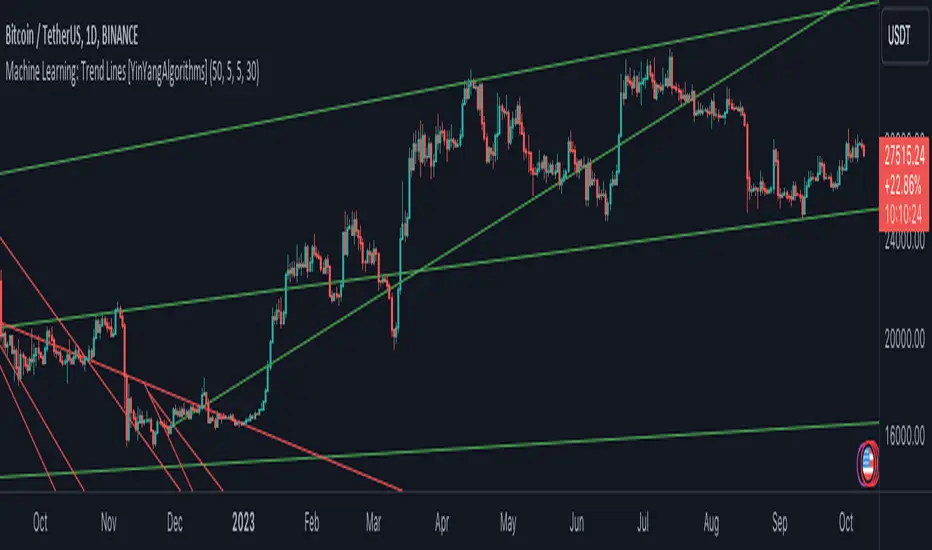
Machine Learning: Trend Lines [YinYangAlgorithms]Trend lines have always been a key indicator that may help predict many different types of price movements. They have been well known to create different types of formations such as: Pennants, Channels, Flags and Wedges. The type of formation they create is based on how the formation was created and the angle it was created. For instance, if there was a strong price increase and then there is a Wedge where both end points meet, this is considered a Bull Pennant. The formations Trend Lines create may be powerful tools that can help predict current Support and Resistance and also Future Momentum changes. However, not all Trend Lines will create formations, and alone they may stand as strong Support and Resistance locations on the Vertical.
The purpose of this Indicator is to apply Machine Learning logic to a Traditional Trend Line Calculation, and therefore allowing a new approach to a modern indicator of high usage. The results of such are quite interesting and goes to show the impacts a simple KNN Machine Learning model can have on Traditional Indicators.
Tutorial:
There are a few different settings within this Indicator. Many will greatly impact the results and if any are changed, lots will need ‘Fine Tuning’. So let's discuss the main toggles that have great effects and what they do before discussing the lengths. Currently in this example above we have the Indicator at its Default Settings. In this example, you can see how the Trend Lines act as key Support and Resistance locations. Due note, Support and Resistance are a relative term, as is their color. What starts off as Support or Resistance may change when the price crosses over / under them.
In the example above we have zoomed in and circled locations that exhibited markers of Support and Resistance along the Trend Lines. These Trend Lines are all created using the Default Settings. As you can see from the example above; just because it is a Green Upwards Trend Line, doesn’t mean it’s a Support Line. Support and Resistance is always shifting on Trend Lines based on the prices location relative to them.
We won’t go through all the Formations Trend Lines make, but the example above, we can see the Trend Lines formed a Downward Channel. Channels are when there are two parallel downwards Trend Lines that are at a relatively similar angle. This means that they won’t ever meet. What may happen when the price is within these channels, is it may bounce between the upper and lower bounds. These Channels may drive the price upwards or downwards, depending on if it is in an Upwards or Downwards Channel.
If you refer to the example above, you’ll notice that the Trend Lines are formed like traditional Trend Lines. They don’t stem from current Highs and Lows but rather Machine Learning Highs and Lows. More often than not, the Machine Learning approach to Trend Lines cause their start point and angle to be quite different than a Traditional Trend Line. Due to this, it may help predict Support and Resistance locations at are more uncommon and therefore can be quite useful.
In the example above we have turned off the toggle in Settings ‘Use Exponential Data Average’. This Settings uses a custom Exponential Data Average of the KNN rather than simply averaging the KNN. By Default it is enabled, but as you can see when it is disabled it may create some pretty strong lasting Trend Lines. This is why we advise you ZOOM OUT AS FAR AS YOU CAN. Trend Lines are only displayed when you’ve zoomed out far enough that their Start Point is visible.
As you can see in this example above, there were 3 major Upward Trend Lines created in 2020 that have had a major impact on Support and Resistance Locations within the last year. Lets zoom in and get a closer look.
We have zoomed in for this example above, and circled some of the major Support and Resistance locations that these Upward Trend Lines may have had a major impact on.
Please note, these Machine Learning Trend Lines aren’t a ‘One Size Fits All’ kind of thing. They are completely customizable within the Settings, so that you can get a tailored experience based on what Pair and Time Frame you are trading on.
When any values are changed within the Settings, you’ll likely need to ‘Fine Tune’ the rest of the settings until your desired result is met. By default the modifiable lengths within the Settings are:
Machine Learning Length: 50
KNN Length:5
Fast ML Data Length: 5
Slow ML Data Length: 30
For example, let's toggle ‘Use Exponential Data Averages’ back on and change ‘Fast ML Data Length’ from 5 to 20 and ‘Slow ML Data Length’ from 30 to 50.
As you can in the example above, all of the lines have changed. Although there are still some strong Support Locations created by the Upwards Trend Lines.
We will conclude our Tutorial here. Hopefully you’ve learned how to use Machine Learning Trend Lines and will be able to now see some more unorthodox Support and Resistance locations on the Vertical.
Settings:
Use Machine Learning Sources: If disabled Traditional Trend line sources (High and Low) will be used rather than Rational Quadratics.
Use KNN Distance Sorting: You can disable this if you wish to not have the Machine Learning Data sorted using KNN. If disabled trend line logic will be Traditional.
Use Exponential Data Average: This Settings uses a custom Exponential Data Average of the KNN rather than simply averaging the KNN.
Machine Learning Length: How strong is our Machine Learning Memory? Please note, when this value is too high the data is almost 'too' much and can lead to poor results.
K-Nearest Neighbour (KNN) Length: How many K-Nearest Neighbours are allowed with our Distance Clustering? Please note, too high or too low may lead to poor results.
Fast ML Data Length: Fast and Slow speed needs to be adjusted properly to see results. 3/5/7 all seem to work well for Fast.
Slow ML Data Length: Fast and Slow speed needs to be adjusted properly to see results. 20 - 50 all seem to work well for Slow.
If you have any questions, comments, ideas or concerns please don't hesitate to contact us.
HAPPY TRADING!
MomentumIndicatorsLibrary "MomentumIndicators"
This is a library of 'Momentum Indicators', also denominated as oscillators.
The purpose of this library is to organize momentum indicators in just one place, making it easy to access.
In addition, it aims to allow customized versions, not being restricted to just the price value.
An example of this use case is the popular Stochastic RSI.
# Indicators:
1. Relative Strength Index (RSI):
Measures the relative strength of recent price gains to recent price losses of an asset.
2. Rate of Change (ROC):
Measures the percentage change in price of an asset over a specified time period.
3. Stochastic Oscillator (Stoch):
Compares the current price of an asset to its price range over a specified time period.
4. True Strength Index (TSI):
Measures the price change, calculating the ratio of the price change (positive or negative) in relation to the
absolute price change.
The values of both are smoothed twice to reduce noise, and the final result is normalized
in a range between 100 and -100.
5. Stochastic Momentum Index (SMI):
Combination of the True Strength Index with a signal line to help identify turning points in the market.
6. Williams Percent Range (Williams %R):
Compares the current price of an asset to its highest high and lowest low over a specified time period.
7. Commodity Channel Index (CCI):
Measures the relationship between an asset's current price and its moving average.
8. Ultimate Oscillator (UO):
Combines three different time periods to help identify possible reversal points.
9. Moving Average Convergence/Divergence (MACD):
Shows the difference between short-term and long-term exponential moving averages.
10. Fisher Transform (FT):
Normalize prices into a Gaussian normal distribution.
11. Inverse Fisher Transform (IFT):
Transform the values of the Fisher Transform into a smaller and more easily interpretable scale is through the
application of an inverse transformation to the hyperbolic tangent function.
This transformation takes the values of the FT, which range from -infinity to +infinity, to a scale limited
between -1 and +1, allowing them to be more easily visualized and compared.
12. Premier Stochastic Oscillator (PSO):
Normalizes the standard stochastic oscillator by applying a five-period double exponential smoothing average of
the %K value, resulting in a symmetric scale of 1 to -1
# Indicators of indicators:
## Stochastic:
1. Stochastic of RSI (Relative Strengh Index)
2. Stochastic of ROC (Rate of Change)
3. Stochastic of UO (Ultimate Oscillator)
4. Stochastic of TSI (True Strengh Index)
5. Stochastic of Williams R%
6. Stochastic of CCI (Commodity Channel Index).
7. Stochastic of MACD (Moving Average Convergence/Divergence)
8. Stochastic of FT (Fisher Transform)
9. Stochastic of Volume
10. Stochastic of MFI (Money Flow Index)
11. Stochastic of On OBV (Balance Volume)
12. Stochastic of PVI (Positive Volume Index)
13. Stochastic of NVI (Negative Volume Index)
14. Stochastic of PVT (Price-Volume Trend)
15. Stochastic of VO (Volume Oscillator)
16. Stochastic of VROC (Volume Rate of Change)
## Inverse Fisher Transform:
1.Inverse Fisher Transform on RSI (Relative Strengh Index)
2.Inverse Fisher Transform on ROC (Rate of Change)
3.Inverse Fisher Transform on UO (Ultimate Oscillator)
4.Inverse Fisher Transform on Stochastic
5.Inverse Fisher Transform on TSI (True Strength Index)
6.Inverse Fisher Transform on CCI (Commodity Channel Index)
7.Inverse Fisher Transform on Fisher Transform (FT)
8.Inverse Fisher Transform on MACD (Moving Average Convergence/Divergence)
9.Inverse Fisher Transfor on Williams R% (Williams Percent Range)
10.Inverse Fisher Transfor on CMF (Chaikin Money Flow)
11.Inverse Fisher Transform on VO (Volume Oscillator)
12.Inverse Fisher Transform on VROC (Volume Rate of Change)
## Stochastic Momentum Index:
1.Stochastic Momentum Index of RSI (Relative Strength Index)
2.Stochastic Momentum Index of ROC (Rate of Change)
3.Stochastic Momentum Index of VROC (Volume Rate of Change)
4.Stochastic Momentum Index of Williams R% (Williams Percent Range)
5.Stochastic Momentum Index of FT (Fisher Transform)
6.Stochastic Momentum Index of CCI (Commodity Channel Index)
7.Stochastic Momentum Index of UO (Ultimate Oscillator)
8.Stochastic Momentum Index of MACD (Moving Average Convergence/Divergence)
9.Stochastic Momentum Index of Volume
10.Stochastic Momentum Index of MFI (Money Flow Index)
11.Stochastic Momentum Index of CMF (Chaikin Money Flow)
12.Stochastic Momentum Index of On Balance Volume (OBV)
13.Stochastic Momentum Index of Price-Volume Trend (PVT)
14.Stochastic Momentum Index of Volume Oscillator (VO)
15.Stochastic Momentum Index of Positive Volume Index (PVI)
16.Stochastic Momentum Index of Negative Volume Index (NVI)
## Relative Strength Index:
1. RSI for Volume
2. RSI for Moving Average
rsi(source, length)
RSI (Relative Strengh Index). Measures the relative strength of recent price gains to recent price losses of an asset.
Parameters:
source : (float) Source of series (close, high, low, etc.)
length : (int) Period of loopback
Returns: (float) Series of RSI
roc(source, length)
ROC (Rate of Change). Measures the percentage change in price of an asset over a specified time period.
Parameters:
source : (float) Source of series (close, high, low, etc.)
length : (int) Period of loopback
Returns: (float) Series of ROC
stoch(kLength, kSmoothing, dSmoothing, maTypeK, maTypeD, almaOffsetKD, almaSigmaKD, lsmaOffSetKD)
Stochastic Oscillator. Compares the current price of an asset to its price range over a specified time period.
Parameters:
kLength
kSmoothing : (int) Period for smoothig stochastic
dSmoothing : (int) Period for signal (moving average of stochastic)
maTypeK : (int) Type of Moving Average for Stochastic Oscillator
maTypeD : (int) Type of Moving Average for Stochastic Oscillator Signal
almaOffsetKD : (float) Offset for Arnaud Legoux Moving Average for Oscillator and Signal
almaSigmaKD : (float) Sigma for Arnaud Legoux Moving Average for Oscillator and Signal
lsmaOffSetKD : (int) Offset for Least Squares Moving Average for Oscillator and Signal
Returns: A tuple of Stochastic Oscillator and Moving Average of Stochastic Oscillator
stoch(source, kLength, kSmoothing, dSmoothing, maTypeK, maTypeD, almaOffsetKD, almaSigmaKD, lsmaOffSetKD)
Stochastic Oscillator. Customized source. Compares the current price of an asset to its price range over a specified time period.
Parameters:
source : (float) Source of series (close, high, low, etc.)
kLength : (int) Period of loopback to calculate the stochastic
kSmoothing : (int) Period for smoothig stochastic
dSmoothing : (int) Period for signal (moving average of stochastic)
maTypeK : (int) Type of Moving Average for Stochastic Oscillator
maTypeD : (int) Type of Moving Average for Stochastic Oscillator Signal
almaOffsetKD : (float) Offset for Arnaud Legoux Moving Average for Stoch and Signal
almaSigmaKD : (float) Sigma for Arnaud Legoux Moving Average for Stoch and Signal
lsmaOffSetKD : (int) Offset for Least Squares Moving Average for Stoch and Signal
Returns: A tuple of Stochastic Oscillator and Moving Average of Stochastic Oscillator
tsi(source, shortLength, longLength, maType, almaOffset, almaSigma, lsmaOffSet)
TSI (True Strengh Index). Measures the price change, calculating the ratio of the price change (positive or negative) in relation to the absolute price change.
The values of both are smoothed twice to reduce noise, and the final result is normalized in a range between 100 and -100.
Parameters:
source : (float) Source of series (close, high, low, etc.)
shortLength : (int) Short length
longLength : (int) Long length
maType : (int) Type of Moving Average for TSI
almaOffset : (float) Offset for Arnaud Legoux Moving Average
almaSigma : (float) Sigma for Arnaud Legoux Moving Average
lsmaOffSet : (int) Offset for Least Squares Moving Average
Returns: (float) TSI
smi(sourceTSI, shortLengthTSI, longLengthTSI, maTypeTSI, almaOffsetTSI, almaSigmaTSI, lsmaOffSetTSI, maTypeSignal, smoothingLengthSignal, almaOffsetSignal, almaSigmaSignal, lsmaOffSetSignal)
SMI (Stochastic Momentum Index). A TSI (True Strengh Index) plus a signal line.
Parameters:
sourceTSI : (float) Source of series for TSI (close, high, low, etc.)
shortLengthTSI : (int) Short length for TSI
longLengthTSI : (int) Long length for TSI
maTypeTSI : (int) Type of Moving Average for Signal of TSI
almaOffsetTSI : (float) Offset for Arnaud Legoux Moving Average
almaSigmaTSI : (float) Sigma for Arnaud Legoux Moving Average
lsmaOffSetTSI : (int) Offset for Least Squares Moving Average
maTypeSignal
smoothingLengthSignal
almaOffsetSignal
almaSigmaSignal
lsmaOffSetSignal
Returns: A tuple with TSI, signal of TSI and histogram of difference
wpr(source, length)
Williams R% (Williams Percent Range). Compares the current price of an asset to its highest high and lowest low over a specified time period.
Parameters:
source : (float) Source of series (close, high, low, etc.)
length : (int) Period of loopback
Returns: (float) Series of Williams R%
cci(source, length, maType, almaOffset, almaSigma, lsmaOffSet)
CCI (Commodity Channel Index). Measures the relationship between an asset's current price and its moving average.
Parameters:
source : (float) Source of series (close, high, low, etc.)
length : (int) Period of loopback
maType : (int) Type of Moving Average
almaOffset : (float) Offset for Arnaud Legoux Moving Average
almaSigma : (float) Sigma for Arnaud Legoux Moving Average
lsmaOffSet : (int) Offset for Least Squares Moving Average
Returns: (float) Series of CCI
ultimateOscillator(fastLength, middleLength, slowLength)
UO (Ultimate Oscilator). Combines three different time periods to help identify possible reversal points.
Parameters:
fastLength : (int) Fast period of loopback
middleLength : (int) Middle period of loopback
slowLength : (int) Slow period of loopback
Returns: (float) Series of Ultimate Oscilator
ultimateOscillator(source, fastLength, middleLength, slowLength)
UO (Ultimate Oscilator). Customized source. Combines three different time periods to help identify possible reversal points.
Parameters:
source : (float) Source of series (close, high, low, etc.)
fastLength : (int) Fast period of loopback
middleLength : (int) Middle period of loopback
slowLength : (int) Slow period of loopback
Returns: (float) Series of Ultimate Oscilator
macd(source, fastLength, slowLength, signalLength, maTypeFast, maTypeSlow, maTypeMACD, almaOffset, almaSigma, lsmaOffSet)
MACD (Moving Average Convergence/Divergence). Shows the difference between short-term and long-term exponential moving averages.
Parameters:
source : (float) Source of series (close, high, low, etc.)
fastLength : (int) Period for fast moving average
slowLength : (int) Period for slow moving average
signalLength : (int) Signal length
maTypeFast : (int) Type of fast moving average
maTypeSlow : (int) Type of slow moving average
maTypeMACD : (int) Type of MACD moving average
almaOffset : (float) Offset for Arnaud Legoux Moving Average
almaSigma : (float) Sigma for Arnaud Legoux Moving Average
lsmaOffSet : (int) Offset for Least Squares Moving Average
Returns: A tuple with MACD, Signal, and Histgram
fisher(length)
Fisher Transform. Normalize prices into a Gaussian normal distribution.
Parameters:
length
Returns: A tuple with Fisher Transform and signal
fisher(source, length)
Fisher Transform. Customized source. Normalize prices into a Gaussian normal distribution.
Parameters:
source : (float) Source of series (close, high, low, etc.)
length
Returns: A tuple with Fisher Transform and signal
inverseFisher(source, length, subtrahend, denominator)
Inverse Fisher Transform.
Transform the values of the Fisher Transform into a smaller and more easily interpretable scale is
through the application of an inverse transformation to the hyperbolic tangent function.
This transformation takes the values of the FT, which range from -infinity to +infinity,
to a scale limited between -1 and +1, allowing them to be more easily visualized and compared.
Parameters:
source : (float) Source of series (close, high, low, etc.)
length : (int) Period for loopback
subtrahend : (int) Denominator. Useful in unbounded indicators. For example, in CCI.
denominator
Returns: (float) Series of Inverse Fisher Transform
premierStoch(length, smoothlen)
Premier Stochastic Oscillator (PSO).
Normalizes the standard stochastic oscillator by applying a five-period double exponential smoothing
average of the %K value, resulting in a symmetric scale of 1 to -1.
Parameters:
length : (int) Period for loopback
smoothlen : (int) Period for smoothing
Returns: (float) Series of PSO
premierStoch(source, smoothlen, subtrahend, denominator)
Premier Stochastic Oscillator (PSO) of custom source.
Normalizes the source by applying a five-period double exponential smoothing average.
Parameters:
source : (float) Source of series (close, high, low, etc.)
smoothlen : (int) Period for smoothing
subtrahend : (int) Denominator. Useful in unbounded indicators. For example, in CCI.
denominator
Returns: (float) Series of PSO
stochRsi(sourceRSI, lengthRSI, kLength, kSmoothing, dSmoothing, maTypeK, maTypeD, almaOffsetKD, almaSigmaKD, lsmaOffSetKD)
Parameters:
sourceRSI
lengthRSI
kLength
kSmoothing
dSmoothing
maTypeK
maTypeD
almaOffsetKD
almaSigmaKD
lsmaOffSetKD
stochRoc(sourceROC, lengthROC, kLength, kSmoothing, dSmoothing, maTypeK, maTypeD, almaOffsetKD, almaSigmaKD, lsmaOffSetKD)
Parameters:
sourceROC
lengthROC
kLength
kSmoothing
dSmoothing
maTypeK
maTypeD
almaOffsetKD
almaSigmaKD
lsmaOffSetKD
stochUO(fastLength, middleLength, slowLength, kLength, kSmoothing, dSmoothing, maTypeK, maTypeD, almaOffsetKD, almaSigmaKD, lsmaOffSetKD)
Parameters:
fastLength
middleLength
slowLength
kLength
kSmoothing
dSmoothing
maTypeK
maTypeD
almaOffsetKD
almaSigmaKD
lsmaOffSetKD
stochTSI(source, shortLength, longLength, maType, almaOffset, almaSigma, lsmaOffSet, kLength, kSmoothing, dSmoothing, maTypeK, maTypeD, almaOffsetKD, almaSigmaKD, lsmaOffSetKD)
Parameters:
source
shortLength
longLength
maType
almaOffset
almaSigma
lsmaOffSet
kLength
kSmoothing
dSmoothing
maTypeK
maTypeD
almaOffsetKD
almaSigmaKD
lsmaOffSetKD
stochWPR(source, length, kLength, kSmoothing, dSmoothing, maTypeK, maTypeD, almaOffsetKD, almaSigmaKD, lsmaOffSetKD)
Parameters:
source
length
kLength
kSmoothing
dSmoothing
maTypeK
maTypeD
almaOffsetKD
almaSigmaKD
lsmaOffSetKD
stochCCI(source, length, maType, almaOffset, almaSigma, lsmaOffSet, kLength, kSmoothing, dSmoothing, maTypeK, maTypeD, almaOffsetKD, almaSigmaKD, lsmaOffSetKD)
Parameters:
source
length
maType
almaOffset
almaSigma
lsmaOffSet
kLength
kSmoothing
dSmoothing
maTypeK
maTypeD
almaOffsetKD
almaSigmaKD
lsmaOffSetKD
stochMACD(source, fastLength, slowLength, signalLength, maTypeFast, maTypeSlow, maTypeMACD, almaOffset, almaSigma, lsmaOffSet, kLength, kSmoothing, dSmoothing, maTypeK, maTypeD, almaOffsetKD, almaSigmaKD, lsmaOffSetKD)
Parameters:
source
fastLength
slowLength
signalLength
maTypeFast
maTypeSlow
maTypeMACD
almaOffset
almaSigma
lsmaOffSet
kLength
kSmoothing
dSmoothing
maTypeK
maTypeD
almaOffsetKD
almaSigmaKD
lsmaOffSetKD
stochFT(length, kLength, kSmoothing, dSmoothing, maTypeK, maTypeD, almaOffsetKD, almaSigmaKD, lsmaOffSetKD)
Parameters:
length
kLength
kSmoothing
dSmoothing
maTypeK
maTypeD
almaOffsetKD
almaSigmaKD
lsmaOffSetKD
stochVolume(kLength, kSmoothing, dSmoothing, maTypeK, maTypeD, almaOffsetKD, almaSigmaKD, lsmaOffSetKD)
Parameters:
kLength
kSmoothing
dSmoothing
maTypeK
maTypeD
almaOffsetKD
almaSigmaKD
lsmaOffSetKD
stochMFI(source, length, kLength, kSmoothing, dSmoothing, maTypeK, maTypeD, almaOffsetKD, almaSigmaKD, lsmaOffSetKD)
Parameters:
source
length
kLength
kSmoothing
dSmoothing
maTypeK
maTypeD
almaOffsetKD
almaSigmaKD
lsmaOffSetKD
stochOBV(source, kLength, kSmoothing, dSmoothing, maTypeK, maTypeD, almaOffsetKD, almaSigmaKD, lsmaOffSetKD)
Parameters:
source
kLength
kSmoothing
dSmoothing
maTypeK
maTypeD
almaOffsetKD
almaSigmaKD
lsmaOffSetKD
stochPVI(source, kLength, kSmoothing, dSmoothing, maTypeK, maTypeD, almaOffsetKD, almaSigmaKD, lsmaOffSetKD)
Parameters:
source
kLength
kSmoothing
dSmoothing
maTypeK
maTypeD
almaOffsetKD
almaSigmaKD
lsmaOffSetKD
stochNVI(source, kLength, kSmoothing, dSmoothing, maTypeK, maTypeD, almaOffsetKD, almaSigmaKD, lsmaOffSetKD)
Parameters:
source
kLength
kSmoothing
dSmoothing
maTypeK
maTypeD
almaOffsetKD
almaSigmaKD
lsmaOffSetKD
stochPVT(source, kLength, kSmoothing, dSmoothing, maTypeK, maTypeD, almaOffsetKD, almaSigmaKD, lsmaOffSetKD)
Parameters:
source
kLength
kSmoothing
dSmoothing
maTypeK
maTypeD
almaOffsetKD
almaSigmaKD
lsmaOffSetKD
stochVO(shortLen, longLen, maType, almaOffset, almaSigma, lsmaOffSet, kLength, kSmoothing, dSmoothing, maTypeK, maTypeD, almaOffsetKD, almaSigmaKD, lsmaOffSetKD)
Parameters:
shortLen
longLen
maType
almaOffset
almaSigma
lsmaOffSet
kLength
kSmoothing
dSmoothing
maTypeK
maTypeD
almaOffsetKD
almaSigmaKD
lsmaOffSetKD
stochVROC(length, kLength, kSmoothing, dSmoothing, maTypeK, maTypeD, almaOffsetKD, almaSigmaKD, lsmaOffSetKD)
Parameters:
length
kLength
kSmoothing
dSmoothing
maTypeK
maTypeD
almaOffsetKD
almaSigmaKD
lsmaOffSetKD
iftRSI(sourceRSI, lengthRSI, lengthIFT)
Parameters:
sourceRSI
lengthRSI
lengthIFT
iftROC(sourceROC, lengthROC, lengthIFT)
Parameters:
sourceROC
lengthROC
lengthIFT
iftUO(fastLength, middleLength, slowLength, lengthIFT)
Parameters:
fastLength
middleLength
slowLength
lengthIFT
iftStoch(kLength, kSmoothing, dSmoothing, maTypeK, maTypeD, almaOffsetKD, almaSigmaKD, lsmaOffSetKD, lengthIFT)
Parameters:
kLength
kSmoothing
dSmoothing
maTypeK
maTypeD
almaOffsetKD
almaSigmaKD
lsmaOffSetKD
lengthIFT
iftTSI(source, shortLength, longLength, maType, almaOffset, almaSigma, lsmaOffSet, lengthIFT)
Parameters:
source
shortLength
longLength
maType
almaOffset
almaSigma
lsmaOffSet
lengthIFT
iftCCI(source, length, maType, almaOffset, almaSigma, lsmaOffSet, lengthIFT)
Parameters:
source
length
maType
almaOffset
almaSigma
lsmaOffSet
lengthIFT
iftFisher(length, lengthIFT)
Parameters:
length
lengthIFT
iftMACD(source, fastLength, slowLength, signalLength, maTypeFast, maTypeSlow, maTypeMACD, almaOffset, almaSigma, lsmaOffSet, lengthIFT)
Parameters:
source
fastLength
slowLength
signalLength
maTypeFast
maTypeSlow
maTypeMACD
almaOffset
almaSigma
lsmaOffSet
lengthIFT
iftWPR(source, length, lengthIFT)
Parameters:
source
length
lengthIFT
iftMFI(source, length, lengthIFT)
Parameters:
source
length
lengthIFT
iftCMF(length, lengthIFT)
Parameters:
length
lengthIFT
iftVO(shortLen, longLen, maType, almaOffset, almaSigma, lsmaOffSet, lengthIFT)
Parameters:
shortLen
longLen
maType
almaOffset
almaSigma
lsmaOffSet
lengthIFT
iftVROC(length, lengthIFT)
Parameters:
length
lengthIFT
smiRSI(source, length, shortLengthTSI, longLengthTSI, maTypeTSI, almaOffsetTSI, almaSigmaTSI, lsmaOffSetTSI, maTypeSignal, smoothingLengthSignal, almaOffsetSignal, almaSigmaSignal, lsmaOffSetSignal)
Parameters:
source
length
shortLengthTSI
longLengthTSI
maTypeTSI
almaOffsetTSI
almaSigmaTSI
lsmaOffSetTSI
maTypeSignal
smoothingLengthSignal
almaOffsetSignal
almaSigmaSignal
lsmaOffSetSignal
smiROC(source, length, shortLengthTSI, longLengthTSI, maTypeTSI, almaOffsetTSI, almaSigmaTSI, lsmaOffSetTSI, maTypeSignal, smoothingLengthSignal, almaOffsetSignal, almaSigmaSignal, lsmaOffSetSignal)
Parameters:
source
length
shortLengthTSI
longLengthTSI
maTypeTSI
almaOffsetTSI
almaSigmaTSI
lsmaOffSetTSI
maTypeSignal
smoothingLengthSignal
almaOffsetSignal
almaSigmaSignal
lsmaOffSetSignal
smiVROC(length, shortLengthTSI, longLengthTSI, maTypeTSI, almaOffsetTSI, almaSigmaTSI, lsmaOffSetTSI, maTypeSignal, smoothingLengthSignal, almaOffsetSignal, almaSigmaSignal, lsmaOffSetSignal)
Parameters:
length
shortLengthTSI
longLengthTSI
maTypeTSI
almaOffsetTSI
almaSigmaTSI
lsmaOffSetTSI
maTypeSignal
smoothingLengthSignal
almaOffsetSignal
almaSigmaSignal
lsmaOffSetSignal
smiWPR(source, length, shortLengthTSI, longLengthTSI, maTypeTSI, almaOffsetTSI, almaSigmaTSI, lsmaOffSetTSI, maTypeSignal, smoothingLengthSignal, almaOffsetSignal, almaSigmaSignal, lsmaOffSetSignal)
Parameters:
source
length
shortLengthTSI
longLengthTSI
maTypeTSI
almaOffsetTSI
almaSigmaTSI
lsmaOffSetTSI
maTypeSignal
smoothingLengthSignal
almaOffsetSignal
almaSigmaSignal
lsmaOffSetSignal
smiFT(length, shortLengthTSI, longLengthTSI, maTypeTSI, almaOffsetTSI, almaSigmaTSI, lsmaOffSetTSI, maTypeSignal, smoothingLengthSignal, almaOffsetSignal, almaSigmaSignal, lsmaOffSetSignal)
Parameters:
length
shortLengthTSI
longLengthTSI
maTypeTSI
almaOffsetTSI
almaSigmaTSI
lsmaOffSetTSI
maTypeSignal
smoothingLengthSignal
almaOffsetSignal
almaSigmaSignal
lsmaOffSetSignal
smiFT(source, length, shortLengthTSI, longLengthTSI, maTypeTSI, almaOffsetTSI, almaSigmaTSI, lsmaOffSetTSI, maTypeSignal, smoothingLengthSignal, almaOffsetSignal, almaSigmaSignal, lsmaOffSetSignal)
Parameters:
source
length
shortLengthTSI
longLengthTSI
maTypeTSI
almaOffsetTSI
almaSigmaTSI
lsmaOffSetTSI
maTypeSignal
smoothingLengthSignal
almaOffsetSignal
almaSigmaSignal
lsmaOffSetSignal
smiCCI(source, length, maTypeCCI, almaOffsetCCI, almaSigmaCCI, lsmaOffSetCCI, shortLengthTSI, longLengthTSI, maTypeTSI, almaOffsetTSI, almaSigmaTSI, lsmaOffSetTSI, maTypeSignal, smoothingLengthSignal, almaOffsetSignal, almaSigmaSignal, lsmaOffSetSignal)
Parameters:
source
length
maTypeCCI
almaOffsetCCI
almaSigmaCCI
lsmaOffSetCCI
shortLengthTSI
longLengthTSI
maTypeTSI
almaOffsetTSI
almaSigmaTSI
lsmaOffSetTSI
maTypeSignal
smoothingLengthSignal
almaOffsetSignal
almaSigmaSignal
lsmaOffSetSignal
smiUO(fastLength, middleLength, slowLength, shortLengthTSI, longLengthTSI, maTypeTSI, almaOffsetTSI, almaSigmaTSI, lsmaOffSetTSI, maTypeSignal, smoothingLengthSignal, almaOffsetSignal, almaSigmaSignal, lsmaOffSetSignal)
Parameters:
fastLength
middleLength
slowLength
shortLengthTSI
longLengthTSI
maTypeTSI
almaOffsetTSI
almaSigmaTSI
lsmaOffSetTSI
maTypeSignal
smoothingLengthSignal
almaOffsetSignal
almaSigmaSignal
lsmaOffSetSignal
smiMACD(source, fastLength, slowLength, signalLength, maTypeFast, maTypeSlow, maTypeMACD, almaOffset, almaSigma, lsmaOffSet, shortLengthTSI, longLengthTSI, maTypeTSI, almaOffsetTSI, almaSigmaTSI, lsmaOffSetTSI, maTypeSignal, smoothingLengthSignal, almaOffsetSignal, almaSigmaSignal, lsmaOffSetSignal)
Parameters:
source
fastLength
slowLength
signalLength
maTypeFast
maTypeSlow
maTypeMACD
almaOffset
almaSigma
lsmaOffSet
shortLengthTSI
longLengthTSI
maTypeTSI
almaOffsetTSI
almaSigmaTSI
lsmaOffSetTSI
maTypeSignal
smoothingLengthSignal
almaOffsetSignal
almaSigmaSignal
lsmaOffSetSignal
smiVol(shortLengthTSI, longLengthTSI, maTypeTSI, almaOffsetTSI, almaSigmaTSI, lsmaOffSetTSI, maTypeSignal, smoothingLengthSignal, almaOffsetSignal, almaSigmaSignal, lsmaOffSetSignal)
Parameters:
shortLengthTSI
longLengthTSI
maTypeTSI
almaOffsetTSI
almaSigmaTSI
lsmaOffSetTSI
maTypeSignal
smoothingLengthSignal
almaOffsetSignal
almaSigmaSignal
lsmaOffSetSignal
smiMFI(source, length, shortLengthTSI, longLengthTSI, maTypeTSI, almaOffsetTSI, almaSigmaTSI, lsmaOffSetTSI, maTypeSignal, smoothingLengthSignal, almaOffsetSignal, almaSigmaSignal, lsmaOffSetSignal)
Parameters:
source
length
shortLengthTSI
longLengthTSI
maTypeTSI
almaOffsetTSI
almaSigmaTSI
lsmaOffSetTSI
maTypeSignal
smoothingLengthSignal
almaOffsetSignal
almaSigmaSignal
lsmaOffSetSignal
smiCMF(length, shortLengthTSI, longLengthTSI, maTypeTSI, almaOffsetTSI, almaSigmaTSI, lsmaOffSetTSI, maTypeSignal, smoothingLengthSignal, almaOffsetSignal, almaSigmaSignal, lsmaOffSetSignal)
Parameters:
length
shortLengthTSI
longLengthTSI
maTypeTSI
almaOffsetTSI
almaSigmaTSI
lsmaOffSetTSI
maTypeSignal
smoothingLengthSignal
almaOffsetSignal
almaSigmaSignal
lsmaOffSetSignal
smiOBV(source, shortLengthTSI, longLengthTSI, maTypeTSI, almaOffsetTSI, almaSigmaTSI, lsmaOffSetTSI, maTypeSignal, smoothingLengthSignal, almaOffsetSignal, almaSigmaSignal, lsmaOffSetSignal)
Parameters:
source
shortLengthTSI
longLengthTSI
maTypeTSI
almaOffsetTSI
almaSigmaTSI
lsmaOffSetTSI
maTypeSignal
smoothingLengthSignal
almaOffsetSignal
almaSigmaSignal
lsmaOffSetSignal
smiPVT(source, shortLengthTSI, longLengthTSI, maTypeTSI, almaOffsetTSI, almaSigmaTSI, lsmaOffSetTSI, maTypeSignal, smoothingLengthSignal, almaOffsetSignal, almaSigmaSignal, lsmaOffSetSignal)
Parameters:
source
shortLengthTSI
longLengthTSI
maTypeTSI
almaOffsetTSI
almaSigmaTSI
lsmaOffSetTSI
maTypeSignal
smoothingLengthSignal
almaOffsetSignal
almaSigmaSignal
lsmaOffSetSignal
smiVO(shortLen, longLen, maType, almaOffset, almaSigma, lsmaOffSet, shortLengthTSI, longLengthTSI, maTypeTSI, almaOffsetTSI, almaSigmaTSI, lsmaOffSetTSI, maTypeSignal, smoothingLengthSignal, almaOffsetSignal, almaSigmaSignal, lsmaOffSetSignal)
Parameters:
shortLen
longLen
maType
almaOffset
almaSigma
lsmaOffSet
shortLengthTSI
longLengthTSI
maTypeTSI
almaOffsetTSI
almaSigmaTSI
lsmaOffSetTSI
maTypeSignal
smoothingLengthSignal
almaOffsetSignal
almaSigmaSignal
lsmaOffSetSignal
smiPVI(source, shortLengthTSI, longLengthTSI, maTypeTSI, almaOffsetTSI, almaSigmaTSI, lsmaOffSetTSI, maTypeSignal, smoothingLengthSignal, almaOffsetSignal, almaSigmaSignal, lsmaOffSetSignal)
Parameters:
source
shortLengthTSI
longLengthTSI
maTypeTSI
almaOffsetTSI
almaSigmaTSI
lsmaOffSetTSI
maTypeSignal
smoothingLengthSignal
almaOffsetSignal
almaSigmaSignal
lsmaOffSetSignal
smiNVI(source, shortLengthTSI, longLengthTSI, maTypeTSI, almaOffsetTSI, almaSigmaTSI, lsmaOffSetTSI, maTypeSignal, smoothingLengthSignal, almaOffsetSignal, almaSigmaSignal, lsmaOffSetSignal)
Parameters:
source
shortLengthTSI
longLengthTSI
maTypeTSI
almaOffsetTSI
almaSigmaTSI
lsmaOffSetTSI
maTypeSignal
smoothingLengthSignal
almaOffsetSignal
almaSigmaSignal
lsmaOffSetSignal
rsiVolume(length)
Parameters:
length
rsiMA(sourceMA, lengthMA, maType, almaOffset, almaSigma, lsmaOffSet, lengthRSI)
Parameters:
sourceMA
lengthMA
maType
almaOffset
almaSigma
lsmaOffSet
lengthRSI
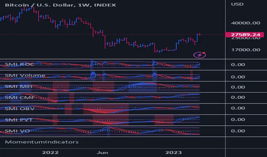
Power Indicator - EMAs + VWAP + Volume BarThe Power Indicator is intended to return some exponential moving average, vwap, volume bar, and others. With this compilation, you will be able to use them as one indicator in Trading View.
The components are:
- EMA9 - Exponential Moving Average of 9 days
- EMA21 - Exponential Moving Average of 21 days
- EMA50 - Exponential Moving Average of 50 days
- EMA200 - Exponential Moving Average of 200 days
- Volume Bar - This indicator provides the volume of the candle and its strength by showing different colors. It's a way to check expressive volume in one bar.
- Vwap line
- Indicator
If you have any questions, let me know!
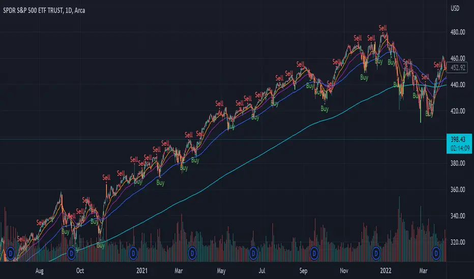
[blackcat] L1 True Range Adjusted EMA (TRAdj EMA) Level: 1
Background
In Traders’ Tips in January 2023, Vitali Apirine published an article in the January 2023 issue, “True Range Adjusted Exponential Moving Average (TRAdj EMA)”.
I use pine v4 to script it.
Function
Vitali Apirine's article True Range Adjusted Exponential Moving Average (TRAdj EMA) presents how a security's True Range, which measures volatility, can be integrated into a traditional exponential moving average. The trend following indicator called True Range Adjusted Exponential Moving Average (TRAdj EMA) applied with different lengths can help define turning points and filter price movements. By comparing the indicator to an exponential moving average of the same length, the trader can gain insight into the overall trend.
Remarks
Feedbacks are appreciated.
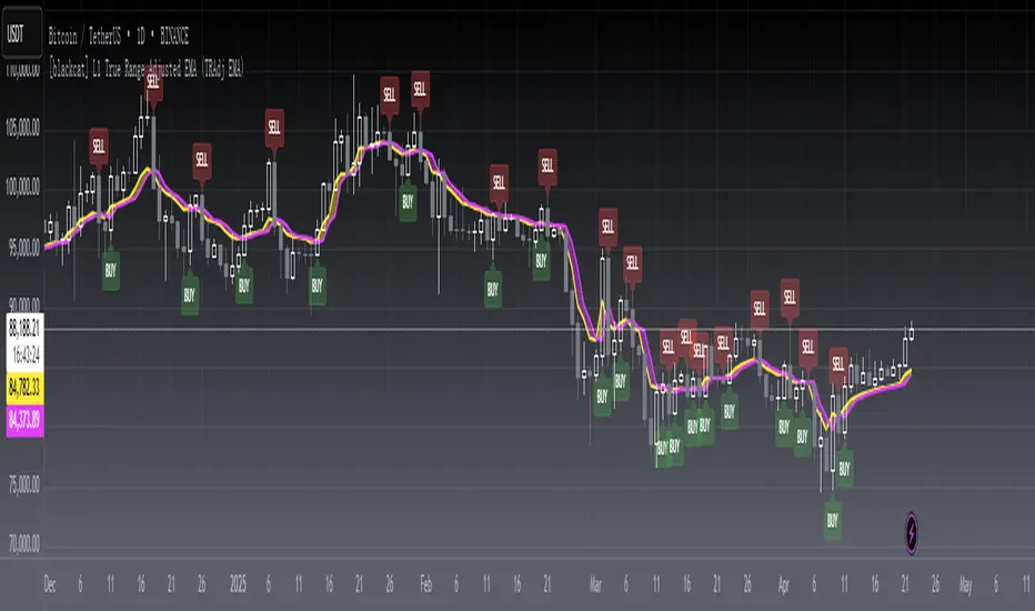
TASC 2022.09 LRAdj EMA█ OVERVIEW
TASC's September 2022 edition of Traders' Tips includes an article by Vitali Apirine titled "The Linear Regression-Adjusted Exponential Moving Average". This script implements the titular indicator presented in this article.
█ CONCEPT
The Linear Regression-Adjusted Exponential Moving Average (LRAdj EMA) is a new tool that combines a linear regression indicator with exponential moving averages . First, the indicator accounts for the linear regression deviation, that is, the distance between the price and the linear regression indicator. Subsequently, an exponential moving average (EMA) smooths the price data and and provides an indication of the current direction.
As part of a trading system, LRAdj EMA can be used in conjunction with an exponential moving average of the same length to identify the overall trend. Alternatively, using LRAdj EMAs of different lengths together can help identify turning points.
█ CALCULATION
The script uses the following input parameters:
EMA Length
LR Lookback Period
Multiplier
The calculation of LRAdj EMA is carried out as follows:
Current LRAdj EMA = Prior LRAdj EMA + MLTP × (1+ LRAdj × Multiplier ) × ( Price − Prior LRAdj EMA ),
where MLTP is a weighting multiplier defined as MLTP = 2 ⁄ ( EMA Length + 1), and LRAdj is the linear regression adjustment (LRAdj) multiplier:
LRAdj = (Abs( Current LR Dist )−Abs( Minimum LR Dist )) ⁄ (Abs( Maximum LR Dist )−Abs( Minimum LR Dist ))
When calculating the LRAdj multiplier, the absolute values of the following quantities are used:
Current LR Dist is the distance between the current close and the linear regression indicator with a length determined by the LR Lookback Period parameter,
Minimum LR Dist is the minimum distance between the close and the linear regression indicator for the LR lookback period ,
Maximum LR Dist is the maximum distance between the close and the linear regression indicator for the LR lookback period .

Rma Stdev BandsStandard Deviation support resistances with percent boxes.
The Relative Moving Average isn’t a well-known moving average. But TradingView uses this average with two popular indicators: the Relative Strength Index (RSI) and Average True Range (ATR)
The weighting factors that the Relative Moving Average uses decrease exponentially. That way recent bars have the highest weight, while earlier bars get smaller weights the older they are.

MovingAveragesLibraryLibrary "MovingAveragesLibrary"
This is a library allowing one to select between many different Moving Average formulas to smooth out any float variable.
You can use this library to apply a Moving Average function to any series of data as long as your source is a float.
The default application would be for applying Moving Averages onto your chart. However, the scope of this library is beyond that. Any indicator or strategy you are building can benefit from this library.
You can apply different types of smoothing and moving average functions to your indicators, momentum oscillators, average true range calculations, support and resistance zones, envelope bands, channels, and anything you can think of to attempt to smooth out noise while finding a delicate balance against lag.
If you are developing an indicator, you can use the 'ave_func' to allow your users to select any Moving Average for any function or variable by creating an input string with the following structure:
var_name = input.string(, , )
Where the types of Moving Average you would like to be provided would be included in options.
Example:
i_ma_type = input.string(title = "Moving Average Type", defval = "Hull Moving Average", options = )
Where you would add after options the strings I have included for you at the top of the PineScript for your convenience.
Then for the output you desire, simply call 'ave_func' like so:
ma = ave_func(source, length, i_ma_type)
Now the plotted Moving Average will be the same as what you or your users select from the Input.
ema(src, len) Exponential Moving Average.
Parameters:
src : Series to use ('close' is used if no argument is supplied).
len : Lookback length to use.
Returns: Float value.
sma(src, len) Simple Moving Average.
Parameters:
src : Series to use ('close' is used if no argument is supplied).
len : Lookback length to use.
Returns: Float value.
rma(src, len) Relative Moving Average.
Parameters:
src : Series to use ('close' is used if no argument is supplied).
len : Lookback length to use.
Returns: Float value.
wma(src, len) Weighted Moving Average.
Parameters:
src : Series to use ('close' is used if no argument is supplied).
len : Lookback length to use.
Returns: Float value.
dv2(len) Donchian V2 function.
Parameters:
len : Lookback length to use.
Returns: Open + Close / 2 for the selected length.
ModFilt(src, len) Modular Filter smoothing function.
Parameters:
src : Series to use ('close' is used if no argument is supplied).
len : Lookback length to use.
Returns: Float value.
EDSMA(src, len) Ehlers Dynamic Smoothed Moving Average.
Parameters:
src : Series to use ('close' is used if no argument is supplied).
len : Lookback length to use.
Returns: EDSMA smoothing.
dema(x, t) Double Exponential Moving Average.
Parameters:
x : Series to use ('close' is used if no argument is supplied).
t : Lookback length to use.
Returns: DEMA smoothing.
tema(src, len) Triple Exponential Moving Average.
Parameters:
src : Series to use ('close' is used if no argument is supplied).
len : Lookback length to use.
Returns: TEMA smoothing.
smma(x, t) Smoothed Moving Average.
Parameters:
x : Series to use ('close' is used if no argument is supplied).
t : Lookback length to use.
Returns: SMMA smoothing.
vwma(x, t) Volume Weighted Moving Average.
Parameters:
x : Series to use ('close' is used if no argument is supplied).
t : Lookback length to use.
Returns: VWMA smoothing.
hullma(x, t) Hull Moving Average.
Parameters:
x : Series to use ('close' is used if no argument is supplied).
t : Lookback length to use.
Returns: Hull smoothing.
covwma(x, t) Coefficient of Variation Weighted Moving Average.
Parameters:
x : Series to use ('close' is used if no argument is supplied).
t : Lookback length to use.
Returns: COVWMA smoothing.
frama(x, t) Fractal Reactive Moving Average.
Parameters:
x : Series to use ('close' is used if no argument is supplied).
t : Lookback length to use.
Returns: FRAMA smoothing.
kama(x, t) Kaufman's Adaptive Moving Average.
Parameters:
x : Series to use ('close' is used if no argument is supplied).
t : Lookback length to use.
Returns: KAMA smoothing.
donchian(len) Donchian Calculation.
Parameters:
len : Lookback length to use.
Returns: Average of the highest price and the lowest price for the specified look-back period.
tma(src, len) Triangular Moving Average.
Parameters:
src : Series to use ('close' is used if no argument is supplied).
len : Lookback length to use.
Returns: TMA smoothing.
VAMA(src, len) Volatility Adjusted Moving Average.
Parameters:
src : Series to use ('close' is used if no argument is supplied).
len : Lookback length to use.
Returns: VAMA smoothing.
Jurik(src, len) Jurik Moving Average.
Parameters:
src : Series to use ('close' is used if no argument is supplied).
len : Lookback length to use.
Returns: JMA smoothing.
MCG(src, len) McGinley smoothing.
Parameters:
src : Series to use ('close' is used if no argument is supplied).
len : Lookback length to use.
Returns: McGinley smoothing.
zlema(series, length) Zero Lag Exponential Moving Average.
Parameters:
series : Series to use ('close' is used if no argument is supplied).
length : Lookback length to use.
Returns: ZLEMA smoothing.
xema(src, len) Optimized Exponential Moving Average.
Parameters:
src : Series to use ('close' is used if no argument is supplied).
len : Lookback length to use.
Returns: XEMA smoothing.
EhlersSuperSmoother(src, lower) Ehlers Super Smoother.
Parameters:
src : Series to use ('close' is used if no argument is supplied).
lower : Smoothing value to use.
Returns: Ehlers Super smoothing.
EhlersEmaSmoother(sig, smoothK, smoothP) Ehlers EMA Smoother.
Parameters:
sig : Series to use ('close' is used if no argument is supplied).
smoothK : Lookback length to use.
smoothP : Smothing value to use.
Returns: Ehlers EMA smoothing.
ave_func(in_src, in_len, in_type) Returns the source after running it through a Moving Average function.
Parameters:
in_src : Series to use ('close' is used if no argument is supplied).
in_len : Lookback period to be used for the Moving Average function.
in_type : Type of Moving Average function to use. Must have a string input to select the options from that MUST match the type-casing in the function below.
Returns: The source as a float after running it through the Moving Average function.

SuperTrended Moving AveragesA different approach to SuperTrend:
adding 100 periods Exponential Moving Average in calculation of SuperTrend and also 0.5 ATR Multiplier to have a clear view of the ongoing trend and also provides significant Supports and Resistances.
Default Moving Average type set as EMA (Exponential Moving Average) but users can choose from 11 different Moving Average types as:
SMA : Simple Moving Average
EMA : Exponential Moving Average
WMA : Weighted Moving Average
DEMA : Double Exponential Moving Average
TMA : Triangular Moving Average
VAR : Variable Index Dynamic Moving Average a.k.a. VIDYA
WWMA : Welles Wilder's Moving Average
ZLEMA : Zero Lag Exponential Moving Average
TSF : True Strength Force
HULL : Hull Moving Average
TILL : Tillson T3 Moving Average
Credits going to @CryptoErge for sharing his development to public.
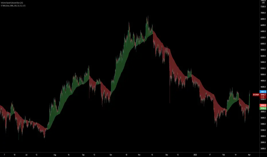
Moving Average Trend█ OVERVIEW
This is a Moving Average Script that contains both a cloud and a ribbon that has independent MA-type selection.
⬆ green arrow up = up trend flip
⬇ red arrow down = down trend flip
🟢 Green Dot = Potential Long
🔴 Red Dot = Potential Short
█ CONCEPTS
1 — Cloud, like most trading algo, the cloud is made of 8 short term MA , with MA cross and MA cross (longema)
2 — Ribbon, this is by default turned off, the default values , an option in setting to change longema to look for ribbon cross
3 — Sequence, It goes from 1 – 9 at 9 the sequence resets. The sequence changes colour depending on if it’s a down trend(red) or uptrend(green) or an over extended trend (yellow)
Setup definitions
Red sell start = current close < the close 4 candles back
Yellow sell extended = current close < last close and current close < two closes back
Green buy start = current close > the close 4 candles back
Yellow buy extended = current close last close and current close < two closes back
This can help you find when it’s time to get out, or sit out of a choppy trend.
4 - Moving Average types:
sma = Simple Moving Average
ema = Exponential Moving Average
wma = Weighted Moving Average
vwma = Volume Weighted Moving Average
rma = Running Moving Average
alma = Arnaud Legoux Moving Average
hma = Hull Moving Average
jma = Jurik Moving Average
frama-o = frama
frama-m = frama mod
dema = Double Exponential Moving Average
tema = Triple Exponential Moving Average
zlema = Zero lag Exponential Moving Average
smma = Smoothed Moving Average
kma = kaufman Moving Average
tma = triangular Moving Average
gmma = Geometric Mean Moving Average
vida = Variable Index Dynamic Average
cma = Corrective Moving average
rema = Range Exponential Moving average
█ OTHER SECTIONS
• FEATURES: to describe the detailed features of the script, usually arranged in the same order as users will find them in the script's inputs.
• HOW TO USE
• LIMITATIONS: Like with any MA script there is a lag factor associated with is.
• RAMBLINGS: Experiment to your hearts content with all the MA types, I'm impartial to HMA as is
• NOTES: some of the MA's are more taxing, therefore take longer to load, be patience, this is a trimmed down version of an existing invite only script i have
MA DerivativesMA Derivatives basicly using Ichimoku Cloud and some additional moving averages for traders.
A. ICHIMOKU
Tenkan-sen (Conversion Line): (9-period high + 9-period low)/2
On a daily chart , this line is the midpoint of the 9-day high-low range, which is almost two weeks.
Kijun-sen (Base Line): (26-period high + 26-period low)/2
On a daily chart , this line is the midpoint of the 26-day high-low range, which is almost one month.
Senkou Span A (Leading Span A): (Conversion Line + Base Line)/2
This is the midpoint between the Conversion Line and the Base Line. The Leading Span A forms one of the two Cloud boundaries. It is referred to as “Leading” because it is plotted 26 periods in the future and forms the faster Cloud boundary.
Senkou Span B (Leading Span B): (52-period high + 52-period low)/2
On the daily chart , this line is the midpoint of the 52-day high-low range, which is a little less than 3 months. The default calculation setting is 52 periods, but it can be adjusted. This value is plotted 26 periods in the future and forms the slower Cloud boundary.
Chikou Span: Represents the closing price and is plotted 26 days back.
Kumo Cloud: Kumo cloud between Senkuo Span A and Senkou Span B lines. It can be green or red. Color can be change with the trend.
You can use Ichimoku for buy&sell strategy
For Buying Strategy
- Tenkansen (Conversion Line) should crossover Kijunsen (Base line) above the highest line of cloud
- Price should be above the highest line of cloud
- Chikouspan should be above the cloud
For Selling Strategy
- Kijunsen (Base Line) should crossover Tenkansen (Conversion Line) below the lowest line of cloud
- Price should be below the lowest line of cloud
- Chikouspan should be below the cloud
B. SIMPLE MOVING AVERAGES
The indicator has some of Simple Moving Averages
It includes:
-Simple Moving Average 50
-Simple Moving Average 100
-Simple Moving Average 200
C. EXPONENTIAL MOVING AVERAGES
The indicator has some of Simple Moving Averages
It includes:
-Exponential Moving Average 9
-Exponential Moving Average 21
-Exponential Moving Average 50
D. BOLLINGER BAND
Bollinger Bands are a type of price envelope developed by John BollingerOpens in a new window. (Price envelopes define upper and lower price range levels.) Bollinger Bands are envelopes plotted at a standard deviation level above and below a simple moving average of the price. Because the distance of the bands is based on standard deviation, they adjust to volatility swings in the underlying price.
Bollinger Bands use 2 parameters, Period and Standard Deviations, StdDev. The default values are 20 for period, and 2 for standard deviations, although you may customize the combinations.
Bollinger bands help determine whether prices are high or low on a relative basis. They are used in pairs, both upper and lower bands and in conjunction with a moving average. Further, the pair of bands is not intended to be used on its own. Use the pair to confirm signals given with other indicators.
How this indicator works
When the bands tighten during a period of low volatility, it raises the likelihood of a sharp price move in either direction. This may begin a trending move. Watch out for a false move in opposite direction which reverses before the proper trend begins.
When the bands separate by an unusual large amount, volatility increases and any existing trend may be ending.
Prices have a tendency to bounce within the bands' envelope, touching one band then moving to the other band. You can use these swings to help identify potential profit targets. For example, if a price bounces off the lower band and then crosses above the moving average, the upper band then becomes the profit target.
Price can exceed or hug a band envelope for prolonged periods during strong trends. On divergence with a momentum oscillator, you may want to do additional research to determine if taking additional profits is appropriate for you.
A strong trend continuation can be expected when the price moves out of the bands. However, if prices move immediately back inside the band, then the suggested strength is negated.
Calculation
First, calculate a simple moving average. Next, calculate the standard deviation over the same number of periods as the simple moving average. For the upper band, add the standard deviation to the moving average. For the lower band, subtract the standard deviation from the moving average.
Typical values used:
Short term: 10 day moving average, bands at 1.5 standard deviations. (1.5 times the standard dev. +/- the SMA)
Medium term: 20 day moving average, bands at 2 standard deviations.
Long term: 50 day moving average, bands at 2.5 standard deviations.
E. ADJUSTABLE MOVING AVERAGES
And this script has also 2 adjustable moving average
- 1 Adjustable Simple Moving Average
- 1 Adjustable Exponential Moving Average
You can just change the length for using this tool.

TrendyIndicator without parameters. The indicator value is the sum of two counters. The first counter adds the ratio (Close/Open) to its previous value if Close > Open. The second counter subtracts from its previous value (Open/Close) if Close < Open. Counters start with zeros. For a larger variance, the ratio is taken exponentially. In general, this is the difference between the number of rising and falling candlesticks.

Grid Like StrategyIt is possible to use progressive position sizing in order to recover from past losses, a well-known position sizing system being the "martingale", which consists of doubling your position size after a loss, this allows you to recover any previous losses in a losing streak + winning an extra. This system has seen a lot of attention from the trading community (mostly from beginners), and many strategies have been designed around the martingale, one of them being "grid trading strategies".
While such strategies often shows promising results on paper, they are often subjects to many frictions during live trading that makes them totally unusable and dangerous to the trader. The motivations behind posting such a strategy isn't to glorify such systems, but rather to present the problems behind them, many users come to me with their ideas and glorious ways to make money, sometimes they present strategies using the martingale, and it is important to present the flaws of this methodology rather than blindly saying "you shouldn't use it".
Strategy Settings
Point determines the "grid" size and should be adjusted accordingly to the scale of the symbol you are applying the strategy to. Higher value would require larger price movements in order to trigger a trade, as such higher values will generate fewer trades.
The order size determines the number of contracts/shares to purchase.
The martingale multiplier determines the factor by which the position size is multiplied after a loss, using values higher to 2 will "squarify" your balance, while a value of 1 would use a constant position sizing.
Finally, the anti-martingale parameter determines whether the strategy uses a reverse martingale or not, if set to true then the position size is multiplied after any wins.
The Grid
Grid strategies are commons and do not present huge problems until we use certain position sizing methods such as the martingale. A martingale is extremely sensitive to any kind of friction (frictional costs, slippage...etc), the grid strategy aims to provide a stable and simple environment where a martingale might possibly behave well.
The goal of a simple grid strategy is to go long once the price crossover a certain level, a take profit is set at the level above the current one and stop loss is placed at the level below the current one, in a winning scenario the price reach the take profit, the position is closed and a new one is opened with the same setup. In a losing scenario, the price reaches the stop loss level, the position is closed and a short one is opened, the take profit is set at the level below the current one, and a stop loss is set at the level above the current one. Note that all levels are equally spaced.
It follows from this strategy that wins and losses should be constant over time, as such our balance would evolve in a linear fashion. This is a great setup for a martingale, as we are theoretically assured to recover all the looses in a losing streak.
Martingale - Exponential Decays - Risk/Reward
By using a martingale we double our position size (exposure) each time we lose a trade, if we look at our balance when using a martingale we see significant drawdowns, with our balance peaking down significantly. The martingale sequence is subject to exponential growth, as such using a martingale makes our balance exposed to exponential decays, that's really bad, we could basically lose all the initially invested capital in a short amount of time, it follows from this that the theoretical success of a martingale is determined by what is the maximum losing streak you can endure
Now consider how a martingale affects our risk-reward ratio, assuming unity position sizing our martingale sequence can be described by 2^(x-1) , using this formula we would get the amount of shares/contracts we need to purchase at the x trade of a losing streak, we would need to purchase 256 contracts in order to recover from a losing streak of size 9, this is enormous when you take into account that your wins are way smaller, the risk-reward ratio is totally unfair.
Of course, some users might think that a losing streak of size 9 is pretty unlikely, if the probability of winning and losing are both equal to 0.5, then the probability of 9 consecutive losses is equal to 0.5^9 , there are approximately 0.2% of chance of having such large losing streak, note however that under a ranging market such case scenario could happen, but we will see later that the length of a losing streak is not the only problem.
Other Problems
Having a capital large enough to tank 9any number of consecutive losses is not the only thing one should focus on, as we have to take into account market prices and trading dynamics, that's where the ugly part start.
Our first problem is frictional costs, one example being the spread, but this is a common problem for any strategy, however here a martingale is extra sensitive to it, if the strategy does not account for it then we will still double our positions costs but we might not recover all the losses of a losing streak, instead we would be recovering only a proportion of it, under such scenario you would be certain to lose over time.
Another problem are gaps, market price might open under a stop-loss without triggering it, and this is a big no-no.
Equity of the strategy on AMD, in a desired scenario the equity at the second arrow should have been at a higher position than the equity at the first arrow.
In order for the strategy to be more effective, we would need to trade a market that does not close, such as the cryptocurrency market. Finally, we might be affected by slippage, altho only extreme values might drastically affect our balance.
The Anti Martingale
The strategy lets you use an anti-martingale, which double the position size after a win instead of a loss, the goal here is not to recover from a losing strike but instead to profit from a potential winning streak.
Here we are exposing your balance to exponential gross but you might also lose a trade at the end a winning streak, you will generally want to reinitialize your position size after a few wins instead of waiting for the end of a streak.
Alternative
You can use other-kind of progressions for position sizing, such as a linear one, increasing your position size by a constant number each time you lose. More gentle progressions will recover a proportion of your losses in a losing streak.
You can also simulate the effect of a martingale without doubling your position size by doubling your target profit, if for example you have a 10$ profit-target/stop-loss and lose a trade, you can use a 20$ profit target to recover from the lost trade + gain a profit of 10$. While this approach does not introduce exponential decay in your balance, you are betting on the market reaching your take profits, considering the fact that you are doubling their size you are expecting market volatility to increase drastically over time, as such this approach would not be extremely effective for high losing streak.
Conclusion
You will see a lot of auto-trading strategies that are based on a grid approach, they might even use a martingale. While the backtests will look appealing, you should think twice before using such kind of strategy, remember that frictional costs will be a huge challenge for the strategy, and that it assumes that the trader has an important initial capital. We have also seen that the risk/reward ratio is theoretically the worst you can have on a strategy, having a low reward and a high risk. This does not mean that progressive position sizing is bad, but it should not be pushed to the extreme.
It is nice to note that the martingale is originally a betting system designed for casino games, which unlike trading are not subject to frictional costs, but even casino players don't use it, so why would you?
Thx for reading

Flying Buddha Inside Bars Indicator v1 by JustUncleLDescription:
=============
This indicator plots MAs and paints Triggered Alert Arrows base on Flying Buddha candle patterns.
The “Flying Buddha” Pattern is defined as:
---------------------------------------------
A candlestick chart with two moving averages: the 5 period exponential moving average (fast EMA) and the 10 period simple moving average (slow SMA), both applied to the closing price. The default “Flying Buddha” pattern is any candlestick which:
1. Has a LOW above the fast EMA, when the fast EMA is above the slow SMA (a bearish “Flying Buddha”); or
2. Has a HIGH below the fast EMA, when the fast EMA is below the slow SMA (a bullish “Flying Buddha”).
Alert Trigger:
---------------
A Flying Buddha Alert is triggered on the first candle that is a non-flying Buddha candle after a Flying Buddha Pattern candle sequence. Flying Buddhas can optionally be filtered by InsideBars and PinBars.
The Alert Trigger is optionally filtered by the Directional MA (default=EMA 89), and/or by Minimum Sequence length of Flying Buddhas.
Moving Averages:
------------------
You can select between 11 different types of moving averages, for each MA line in Flying Buddha MAs (fastMA and slowMA) and the Directional Filter MA:
SMA = Simple Moving Average.
EMA = Exponential Moving Average.
WMA = Weighted Moving Average
VWMA = Volume Weighted Moving Average
SMMA = Smoothed Simple Moving Average.
DEMA = Double Exponential Moving Average
TEMA = Triple Exponential Moving Average.
HullMA = Hull Moving Average
SSMA = Ehlers Super Smoother Moving average
ZEMA = Near Zero Lag Exponential Moving Average.
TMA = Triangular (smoothed) Simple Moving Average.
NOTE: This is a concept indicator, I also intend to release a trading BOT suitable for Autoview, based on this concept indicator.

Fib Guppy for volatility predictionsThis is a guppy made from FIbbonacci numbers (from 1 to 1597).
Here is how to trade with this guppy.
when 6-8 lines tighten together, it means there will be high volatility coming very soon. Trade according to where the next candle opens (for scalping etc). For example: if the 8 lines of guppy tighten and candle closes above guppy with momentum and trend in the same direction(up), then there could be expected a big move in that direction. Vice versa if a candle closes below the tightened guppy with momentum and trend at the same direction, then the volatility will push price lower exponentially.
Easy. peace of cake. go make yourself a millionaire.
Moving Average RibbonThis is an extension of the Madrid Moving Average Ribbon public script to allow for different kinds of moving averages (the original allows only exponential and simple). Possible entries in the MA Type argument field are:
sma (simple moving average)
ema (exponential moving average)
wma (weighted moving average)
trima (triangular moving average)
zlema (zero-lag exponential moving average)
dema (double exponential moving average)
tema (triple exponential moving average)
hma (hull moving average)
If the argument given by the user does not match anything from the above list, it will default to ema.