RCI3lines3 lines RCI
Original author is Jadbrother and modified for 3 lines, 9,35,52, by gero on Jun.29 2016.
Cari skrip untuk "2016年黄金价格"
Markov Chain [3D] | FractalystWhat exactly is a Markov Chain?
This indicator uses a Markov Chain model to analyze, quantify, and visualize the transitions between market regimes (Bull, Bear, Neutral) on your chart. It dynamically detects these regimes in real-time, calculates transition probabilities, and displays them as animated 3D spheres and arrows, giving traders intuitive insight into current and future market conditions.
How does a Markov Chain work, and how should I read this spheres-and-arrows diagram?
Think of three weather modes: Sunny, Rainy, Cloudy.
Each sphere is one mode. The loop on a sphere means “stay the same next step” (e.g., Sunny again tomorrow).
The arrows leaving a sphere show where things usually go next if they change (e.g., Sunny moving to Cloudy).
Some paths matter more than others. A more prominent loop means the current mode tends to persist. A more prominent outgoing arrow means a change to that destination is the usual next step.
Direction isn’t symmetric: moving Sunny→Cloudy can behave differently than Cloudy→Sunny.
Now relabel the spheres to markets: Bull, Bear, Neutral.
Spheres: market regimes (uptrend, downtrend, range).
Self‑loop: tendency for the current regime to continue on the next bar.
Arrows: the most common next regime if a switch happens.
How to read: Start at the sphere that matches current bar state. If the loop stands out, expect continuation. If one outgoing path stands out, that switch is the typical next step. Opposite directions can differ (Bear→Neutral doesn’t have to match Neutral→Bear).
What states and transitions are shown?
The three market states visualized are:
Bullish (Bull): Upward or strong-market regime.
Bearish (Bear): Downward or weak-market regime.
Neutral: Sideways or range-bound regime.
Bidirectional animated arrows and probability labels show how likely the market is to move from one regime to another (e.g., Bull → Bear or Neutral → Bull).
How does the regime detection system work?
You can use either built-in price returns (based on adaptive Z-score normalization) or supply three custom indicators (such as volume, oscillators, etc.).
Values are statistically normalized (Z-scored) over a configurable lookback period.
The normalized outputs are classified into Bull, Bear, or Neutral zones.
If using three indicators, their regime signals are averaged and smoothed for robustness.
How are transition probabilities calculated?
On every confirmed bar, the algorithm tracks the sequence of detected market states, then builds a rolling window of transitions.
The code maintains a transition count matrix for all regime pairs (e.g., Bull → Bear).
Transition probabilities are extracted for each possible state change using Laplace smoothing for numerical stability, and frequently updated in real-time.
What is unique about the visualization?
3D animated spheres represent each regime and change visually when active.
Animated, bidirectional arrows reveal transition probabilities and allow you to see both dominant and less likely regime flows.
Particles (moving dots) animate along the arrows, enhancing the perception of regime flow direction and speed.
All elements dynamically update with each new price bar, providing a live market map in an intuitive, engaging format.
Can I use custom indicators for regime classification?
Yes! Enable the "Custom Indicators" switch and select any three chart series as inputs. These will be normalized and combined (each with equal weight), broadening the regime classification beyond just price-based movement.
What does the “Lookback Period” control?
Lookback Period (default: 100) sets how much historical data builds the probability matrix. Shorter periods adapt faster to regime changes but may be noisier. Longer periods are more stable but slower to adapt.
How is this different from a Hidden Markov Model (HMM)?
It sets the window for both regime detection and probability calculations. Lower values make the system more reactive, but potentially noisier. Higher values smooth estimates and make the system more robust.
How is this Markov Chain different from a Hidden Markov Model (HMM)?
Markov Chain (as here): All market regimes (Bull, Bear, Neutral) are directly observable on the chart. The transition matrix is built from actual detected regimes, keeping the model simple and interpretable.
Hidden Markov Model: The actual regimes are unobservable ("hidden") and must be inferred from market output or indicator "emissions" using statistical learning algorithms. HMMs are more complex, can capture more subtle structure, but are harder to visualize and require additional machine learning steps for training.
A standard Markov Chain models transitions between observable states using a simple transition matrix, while a Hidden Markov Model assumes the true states are hidden (latent) and must be inferred from observable “emissions” like price or volume data. In practical terms, a Markov Chain is transparent and easier to implement and interpret; an HMM is more expressive but requires statistical inference to estimate hidden states from data.
Markov Chain: states are observable; you directly count or estimate transition probabilities between visible states. This makes it simpler, faster, and easier to validate and tune.
HMM: states are hidden; you only observe emissions generated by those latent states. Learning involves machine learning/statistical algorithms (commonly Baum–Welch/EM for training and Viterbi for decoding) to infer both the transition dynamics and the most likely hidden state sequence from data.
How does the indicator avoid “repainting” or look-ahead bias?
All regime changes and matrix updates happen only on confirmed (closed) bars, so no future data is leaked, ensuring reliable real-time operation.
Are there practical tuning tips?
Tune the Lookback Period for your asset/timeframe: shorter for fast markets, longer for stability.
Use custom indicators if your asset has unique regime drivers.
Watch for rapid changes in transition probabilities as early warning of a possible regime shift.
Who is this indicator for?
Quants and quantitative researchers exploring probabilistic market modeling, especially those interested in regime-switching dynamics and Markov models.
Programmers and system developers who need a probabilistic regime filter for systematic and algorithmic backtesting:
The Markov Chain indicator is ideally suited for programmatic integration via its bias output (1 = Bull, 0 = Neutral, -1 = Bear).
Although the visualization is engaging, the core output is designed for automated, rules-based workflows—not for discretionary/manual trading decisions.
Developers can connect the indicator’s output directly to their Pine Script logic (using input.source()), allowing rapid and robust backtesting of regime-based strategies.
It acts as a plug-and-play regime filter: simply plug the bias output into your entry/exit logic, and you have a scientifically robust, probabilistically-derived signal for filtering, timing, position sizing, or risk regimes.
The MC's output is intentionally "trinary" (1/0/-1), focusing on clear regime states for unambiguous decision-making in code. If you require nuanced, multi-probability or soft-label state vectors, consider expanding the indicator or stacking it with a probability-weighted logic layer in your scripting.
Because it avoids subjectivity, this approach is optimal for systematic quants, algo developers building backtested, repeatable strategies based on probabilistic regime analysis.
What's the mathematical foundation behind this?
The mathematical foundation behind this Markov Chain indicator—and probabilistic regime detection in finance—draws from two principal models: the (standard) Markov Chain and the Hidden Markov Model (HMM).
How to use this indicator programmatically?
The Markov Chain indicator automatically exports a bias value (+1 for Bullish, -1 for Bearish, 0 for Neutral) as a plot visible in the Data Window. This allows you to integrate its regime signal into your own scripts and strategies for backtesting, automation, or live trading.
Step-by-Step Integration with Pine Script (input.source)
Add the Markov Chain indicator to your chart.
This must be done first, since your custom script will "pull" the bias signal from the indicator's plot.
In your strategy, create an input using input.source()
Example:
//@version=5
strategy("MC Bias Strategy Example")
mcBias = input.source(close, "MC Bias Source")
After saving, go to your script’s settings. For the “MC Bias Source” input, select the plot/output of the Markov Chain indicator (typically its bias plot).
Use the bias in your trading logic
Example (long only on Bull, flat otherwise):
if mcBias == 1
strategy.entry("Long", strategy.long)
else
strategy.close("Long")
For more advanced workflows, combine mcBias with additional filters or trailing stops.
How does this work behind-the-scenes?
TradingView’s input.source() lets you use any plot from another indicator as a real-time, “live” data feed in your own script (source).
The selected bias signal is available to your Pine code as a variable, enabling logical decisions based on regime (trend-following, mean-reversion, etc.).
This enables powerful strategy modularity : decouple regime detection from entry/exit logic, allowing fast experimentation without rewriting core signal code.
Integrating 45+ Indicators with Your Markov Chain — How & Why
The Enhanced Custom Indicators Export script exports a massive suite of over 45 technical indicators—ranging from classic momentum (RSI, MACD, Stochastic, etc.) to trend, volume, volatility, and oscillator tools—all pre-calculated, centered/scaled, and available as plots.
// Enhanced Custom Indicators Export - 45 Technical Indicators
// Comprehensive technical analysis suite for advanced market regime detection
//@version=6
indicator('Enhanced Custom Indicators Export | Fractalyst', shorttitle='Enhanced CI Export', overlay=false, scale=scale.right, max_labels_count=500, max_lines_count=500)
// |----- Input Parameters -----| //
momentum_group = "Momentum Indicators"
trend_group = "Trend Indicators"
volume_group = "Volume Indicators"
volatility_group = "Volatility Indicators"
oscillator_group = "Oscillator Indicators"
display_group = "Display Settings"
// Common lengths
length_14 = input.int(14, "Standard Length (14)", minval=1, maxval=100, group=momentum_group)
length_20 = input.int(20, "Medium Length (20)", minval=1, maxval=200, group=trend_group)
length_50 = input.int(50, "Long Length (50)", minval=1, maxval=200, group=trend_group)
// Display options
show_table = input.bool(true, "Show Values Table", group=display_group)
table_size = input.string("Small", "Table Size", options= , group=display_group)
// |----- MOMENTUM INDICATORS (15 indicators) -----| //
// 1. RSI (Relative Strength Index)
rsi_14 = ta.rsi(close, length_14)
rsi_centered = rsi_14 - 50
// 2. Stochastic Oscillator
stoch_k = ta.stoch(close, high, low, length_14)
stoch_d = ta.sma(stoch_k, 3)
stoch_centered = stoch_k - 50
// 3. Williams %R
williams_r = ta.stoch(close, high, low, length_14) - 100
// 4. MACD (Moving Average Convergence Divergence)
= ta.macd(close, 12, 26, 9)
// 5. Momentum (Rate of Change)
momentum = ta.mom(close, length_14)
momentum_pct = (momentum / close ) * 100
// 6. Rate of Change (ROC)
roc = ta.roc(close, length_14)
// 7. Commodity Channel Index (CCI)
cci = ta.cci(close, length_20)
// 8. Money Flow Index (MFI)
mfi = ta.mfi(close, length_14)
mfi_centered = mfi - 50
// 9. Awesome Oscillator (AO)
ao = ta.sma(hl2, 5) - ta.sma(hl2, 34)
// 10. Accelerator Oscillator (AC)
ac = ao - ta.sma(ao, 5)
// 11. Chande Momentum Oscillator (CMO)
cmo = ta.cmo(close, length_14)
// 12. Detrended Price Oscillator (DPO)
dpo = close - ta.sma(close, length_20)
// 13. Price Oscillator (PPO)
ppo = ta.sma(close, 12) - ta.sma(close, 26)
ppo_pct = (ppo / ta.sma(close, 26)) * 100
// 14. TRIX
trix_ema1 = ta.ema(close, length_14)
trix_ema2 = ta.ema(trix_ema1, length_14)
trix_ema3 = ta.ema(trix_ema2, length_14)
trix = ta.roc(trix_ema3, 1) * 10000
// 15. Klinger Oscillator
klinger = ta.ema(volume * (high + low + close) / 3, 34) - ta.ema(volume * (high + low + close) / 3, 55)
// 16. Fisher Transform
fisher_hl2 = 0.5 * (hl2 - ta.lowest(hl2, 10)) / (ta.highest(hl2, 10) - ta.lowest(hl2, 10)) - 0.25
fisher = 0.5 * math.log((1 + fisher_hl2) / (1 - fisher_hl2))
// 17. Stochastic RSI
stoch_rsi = ta.stoch(rsi_14, rsi_14, rsi_14, length_14)
stoch_rsi_centered = stoch_rsi - 50
// 18. Relative Vigor Index (RVI)
rvi_num = ta.swma(close - open)
rvi_den = ta.swma(high - low)
rvi = rvi_den != 0 ? rvi_num / rvi_den : 0
// 19. Balance of Power (BOP)
bop = (close - open) / (high - low)
// |----- TREND INDICATORS (10 indicators) -----| //
// 20. Simple Moving Average Momentum
sma_20 = ta.sma(close, length_20)
sma_momentum = ((close - sma_20) / sma_20) * 100
// 21. Exponential Moving Average Momentum
ema_20 = ta.ema(close, length_20)
ema_momentum = ((close - ema_20) / ema_20) * 100
// 22. Parabolic SAR
sar = ta.sar(0.02, 0.02, 0.2)
sar_trend = close > sar ? 1 : -1
// 23. Linear Regression Slope
lr_slope = ta.linreg(close, length_20, 0) - ta.linreg(close, length_20, 1)
// 24. Moving Average Convergence (MAC)
mac = ta.sma(close, 10) - ta.sma(close, 30)
// 25. Trend Intensity Index (TII)
tii_sum = 0.0
for i = 1 to length_20
tii_sum += close > close ? 1 : 0
tii = (tii_sum / length_20) * 100
// 26. Ichimoku Cloud Components
ichimoku_tenkan = (ta.highest(high, 9) + ta.lowest(low, 9)) / 2
ichimoku_kijun = (ta.highest(high, 26) + ta.lowest(low, 26)) / 2
ichimoku_signal = ichimoku_tenkan > ichimoku_kijun ? 1 : -1
// 27. MESA Adaptive Moving Average (MAMA)
mama_alpha = 2.0 / (length_20 + 1)
mama = ta.ema(close, length_20)
mama_momentum = ((close - mama) / mama) * 100
// 28. Zero Lag Exponential Moving Average (ZLEMA)
zlema_lag = math.round((length_20 - 1) / 2)
zlema_data = close + (close - close )
zlema = ta.ema(zlema_data, length_20)
zlema_momentum = ((close - zlema) / zlema) * 100
// |----- VOLUME INDICATORS (6 indicators) -----| //
// 29. On-Balance Volume (OBV)
obv = ta.obv
// 30. Volume Rate of Change (VROC)
vroc = ta.roc(volume, length_14)
// 31. Price Volume Trend (PVT)
pvt = ta.pvt
// 32. Negative Volume Index (NVI)
nvi = 0.0
nvi := volume < volume ? nvi + ((close - close ) / close ) * nvi : nvi
// 33. Positive Volume Index (PVI)
pvi = 0.0
pvi := volume > volume ? pvi + ((close - close ) / close ) * pvi : pvi
// 34. Volume Oscillator
vol_osc = ta.sma(volume, 5) - ta.sma(volume, 10)
// 35. Ease of Movement (EOM)
eom_distance = high - low
eom_box_height = volume / 1000000
eom = eom_box_height != 0 ? eom_distance / eom_box_height : 0
eom_sma = ta.sma(eom, length_14)
// 36. Force Index
force_index = volume * (close - close )
force_index_sma = ta.sma(force_index, length_14)
// |----- VOLATILITY INDICATORS (10 indicators) -----| //
// 37. Average True Range (ATR)
atr = ta.atr(length_14)
atr_pct = (atr / close) * 100
// 38. Bollinger Bands Position
bb_basis = ta.sma(close, length_20)
bb_dev = 2.0 * ta.stdev(close, length_20)
bb_upper = bb_basis + bb_dev
bb_lower = bb_basis - bb_dev
bb_position = bb_dev != 0 ? (close - bb_basis) / bb_dev : 0
bb_width = bb_dev != 0 ? (bb_upper - bb_lower) / bb_basis * 100 : 0
// 39. Keltner Channels Position
kc_basis = ta.ema(close, length_20)
kc_range = ta.ema(ta.tr, length_20)
kc_upper = kc_basis + (2.0 * kc_range)
kc_lower = kc_basis - (2.0 * kc_range)
kc_position = kc_range != 0 ? (close - kc_basis) / kc_range : 0
// 40. Donchian Channels Position
dc_upper = ta.highest(high, length_20)
dc_lower = ta.lowest(low, length_20)
dc_basis = (dc_upper + dc_lower) / 2
dc_position = (dc_upper - dc_lower) != 0 ? (close - dc_basis) / (dc_upper - dc_lower) : 0
// 41. Standard Deviation
std_dev = ta.stdev(close, length_20)
std_dev_pct = (std_dev / close) * 100
// 42. Relative Volatility Index (RVI)
rvi_up = ta.stdev(close > close ? close : 0, length_14)
rvi_down = ta.stdev(close < close ? close : 0, length_14)
rvi_total = rvi_up + rvi_down
rvi_volatility = rvi_total != 0 ? (rvi_up / rvi_total) * 100 : 50
// 43. Historical Volatility
hv_returns = math.log(close / close )
hv = ta.stdev(hv_returns, length_20) * math.sqrt(252) * 100
// 44. Garman-Klass Volatility
gk_vol = math.log(high/low) * math.log(high/low) - (2*math.log(2)-1) * math.log(close/open) * math.log(close/open)
gk_volatility = math.sqrt(ta.sma(gk_vol, length_20)) * 100
// 45. Parkinson Volatility
park_vol = math.log(high/low) * math.log(high/low)
parkinson = math.sqrt(ta.sma(park_vol, length_20) / (4 * math.log(2))) * 100
// 46. Rogers-Satchell Volatility
rs_vol = math.log(high/close) * math.log(high/open) + math.log(low/close) * math.log(low/open)
rogers_satchell = math.sqrt(ta.sma(rs_vol, length_20)) * 100
// |----- OSCILLATOR INDICATORS (5 indicators) -----| //
// 47. Elder Ray Index
elder_bull = high - ta.ema(close, 13)
elder_bear = low - ta.ema(close, 13)
elder_power = elder_bull + elder_bear
// 48. Schaff Trend Cycle (STC)
stc_macd = ta.ema(close, 23) - ta.ema(close, 50)
stc_k = ta.stoch(stc_macd, stc_macd, stc_macd, 10)
stc_d = ta.ema(stc_k, 3)
stc = ta.stoch(stc_d, stc_d, stc_d, 10)
// 49. Coppock Curve
coppock_roc1 = ta.roc(close, 14)
coppock_roc2 = ta.roc(close, 11)
coppock = ta.wma(coppock_roc1 + coppock_roc2, 10)
// 50. Know Sure Thing (KST)
kst_roc1 = ta.roc(close, 10)
kst_roc2 = ta.roc(close, 15)
kst_roc3 = ta.roc(close, 20)
kst_roc4 = ta.roc(close, 30)
kst = ta.sma(kst_roc1, 10) + 2*ta.sma(kst_roc2, 10) + 3*ta.sma(kst_roc3, 10) + 4*ta.sma(kst_roc4, 15)
// 51. Percentage Price Oscillator (PPO)
ppo_line = ((ta.ema(close, 12) - ta.ema(close, 26)) / ta.ema(close, 26)) * 100
ppo_signal = ta.ema(ppo_line, 9)
ppo_histogram = ppo_line - ppo_signal
// |----- PLOT MAIN INDICATORS -----| //
// Plot key momentum indicators
plot(rsi_centered, title="01_RSI_Centered", color=color.purple, linewidth=1)
plot(stoch_centered, title="02_Stoch_Centered", color=color.blue, linewidth=1)
plot(williams_r, title="03_Williams_R", color=color.red, linewidth=1)
plot(macd_histogram, title="04_MACD_Histogram", color=color.orange, linewidth=1)
plot(cci, title="05_CCI", color=color.green, linewidth=1)
// Plot trend indicators
plot(sma_momentum, title="06_SMA_Momentum", color=color.navy, linewidth=1)
plot(ema_momentum, title="07_EMA_Momentum", color=color.maroon, linewidth=1)
plot(sar_trend, title="08_SAR_Trend", color=color.teal, linewidth=1)
plot(lr_slope, title="09_LR_Slope", color=color.lime, linewidth=1)
plot(mac, title="10_MAC", color=color.fuchsia, linewidth=1)
// Plot volatility indicators
plot(atr_pct, title="11_ATR_Pct", color=color.yellow, linewidth=1)
plot(bb_position, title="12_BB_Position", color=color.aqua, linewidth=1)
plot(kc_position, title="13_KC_Position", color=color.olive, linewidth=1)
plot(std_dev_pct, title="14_StdDev_Pct", color=color.silver, linewidth=1)
plot(bb_width, title="15_BB_Width", color=color.gray, linewidth=1)
// Plot volume indicators
plot(vroc, title="16_VROC", color=color.blue, linewidth=1)
plot(eom_sma, title="17_EOM", color=color.red, linewidth=1)
plot(vol_osc, title="18_Vol_Osc", color=color.green, linewidth=1)
plot(force_index_sma, title="19_Force_Index", color=color.orange, linewidth=1)
plot(obv, title="20_OBV", color=color.purple, linewidth=1)
// Plot additional oscillators
plot(ao, title="21_Awesome_Osc", color=color.navy, linewidth=1)
plot(cmo, title="22_CMO", color=color.maroon, linewidth=1)
plot(dpo, title="23_DPO", color=color.teal, linewidth=1)
plot(trix, title="24_TRIX", color=color.lime, linewidth=1)
plot(fisher, title="25_Fisher", color=color.fuchsia, linewidth=1)
// Plot more momentum indicators
plot(mfi_centered, title="26_MFI_Centered", color=color.yellow, linewidth=1)
plot(ac, title="27_AC", color=color.aqua, linewidth=1)
plot(ppo_pct, title="28_PPO_Pct", color=color.olive, linewidth=1)
plot(stoch_rsi_centered, title="29_StochRSI_Centered", color=color.silver, linewidth=1)
plot(klinger, title="30_Klinger", color=color.gray, linewidth=1)
// Plot trend continuation
plot(tii, title="31_TII", color=color.blue, linewidth=1)
plot(ichimoku_signal, title="32_Ichimoku_Signal", color=color.red, linewidth=1)
plot(mama_momentum, title="33_MAMA_Momentum", color=color.green, linewidth=1)
plot(zlema_momentum, title="34_ZLEMA_Momentum", color=color.orange, linewidth=1)
plot(bop, title="35_BOP", color=color.purple, linewidth=1)
// Plot volume continuation
plot(nvi, title="36_NVI", color=color.navy, linewidth=1)
plot(pvi, title="37_PVI", color=color.maroon, linewidth=1)
plot(momentum_pct, title="38_Momentum_Pct", color=color.teal, linewidth=1)
plot(roc, title="39_ROC", color=color.lime, linewidth=1)
plot(rvi, title="40_RVI", color=color.fuchsia, linewidth=1)
// Plot volatility continuation
plot(dc_position, title="41_DC_Position", color=color.yellow, linewidth=1)
plot(rvi_volatility, title="42_RVI_Volatility", color=color.aqua, linewidth=1)
plot(hv, title="43_Historical_Vol", color=color.olive, linewidth=1)
plot(gk_volatility, title="44_GK_Volatility", color=color.silver, linewidth=1)
plot(parkinson, title="45_Parkinson_Vol", color=color.gray, linewidth=1)
// Plot final oscillators
plot(rogers_satchell, title="46_RS_Volatility", color=color.blue, linewidth=1)
plot(elder_power, title="47_Elder_Power", color=color.red, linewidth=1)
plot(stc, title="48_STC", color=color.green, linewidth=1)
plot(coppock, title="49_Coppock", color=color.orange, linewidth=1)
plot(kst, title="50_KST", color=color.purple, linewidth=1)
// Plot final indicators
plot(ppo_histogram, title="51_PPO_Histogram", color=color.navy, linewidth=1)
plot(pvt, title="52_PVT", color=color.maroon, linewidth=1)
// |----- Reference Lines -----| //
hline(0, "Zero Line", color=color.gray, linestyle=hline.style_dashed, linewidth=1)
hline(50, "Midline", color=color.gray, linestyle=hline.style_dotted, linewidth=1)
hline(-50, "Lower Midline", color=color.gray, linestyle=hline.style_dotted, linewidth=1)
hline(25, "Upper Threshold", color=color.gray, linestyle=hline.style_dotted, linewidth=1)
hline(-25, "Lower Threshold", color=color.gray, linestyle=hline.style_dotted, linewidth=1)
// |----- Enhanced Information Table -----| //
if show_table and barstate.islast
table_position = position.top_right
table_text_size = table_size == "Tiny" ? size.tiny : table_size == "Small" ? size.small : size.normal
var table info_table = table.new(table_position, 3, 18, bgcolor=color.new(color.white, 85), border_width=1, border_color=color.gray)
// Headers
table.cell(info_table, 0, 0, 'Category', text_color=color.black, text_size=table_text_size, bgcolor=color.new(color.blue, 70))
table.cell(info_table, 1, 0, 'Indicator', text_color=color.black, text_size=table_text_size, bgcolor=color.new(color.blue, 70))
table.cell(info_table, 2, 0, 'Value', text_color=color.black, text_size=table_text_size, bgcolor=color.new(color.blue, 70))
// Key Momentum Indicators
table.cell(info_table, 0, 1, 'MOMENTUM', text_color=color.purple, text_size=table_text_size, bgcolor=color.new(color.purple, 90))
table.cell(info_table, 1, 1, 'RSI Centered', text_color=color.purple, text_size=table_text_size)
table.cell(info_table, 2, 1, str.tostring(rsi_centered, '0.00'), text_color=color.purple, text_size=table_text_size)
table.cell(info_table, 0, 2, '', text_color=color.blue, text_size=table_text_size)
table.cell(info_table, 1, 2, 'Stoch Centered', text_color=color.blue, text_size=table_text_size)
table.cell(info_table, 2, 2, str.tostring(stoch_centered, '0.00'), text_color=color.blue, text_size=table_text_size)
table.cell(info_table, 0, 3, '', text_color=color.red, text_size=table_text_size)
table.cell(info_table, 1, 3, 'Williams %R', text_color=color.red, text_size=table_text_size)
table.cell(info_table, 2, 3, str.tostring(williams_r, '0.00'), text_color=color.red, text_size=table_text_size)
table.cell(info_table, 0, 4, '', text_color=color.orange, text_size=table_text_size)
table.cell(info_table, 1, 4, 'MACD Histogram', text_color=color.orange, text_size=table_text_size)
table.cell(info_table, 2, 4, str.tostring(macd_histogram, '0.000'), text_color=color.orange, text_size=table_text_size)
table.cell(info_table, 0, 5, '', text_color=color.green, text_size=table_text_size)
table.cell(info_table, 1, 5, 'CCI', text_color=color.green, text_size=table_text_size)
table.cell(info_table, 2, 5, str.tostring(cci, '0.00'), text_color=color.green, text_size=table_text_size)
// Key Trend Indicators
table.cell(info_table, 0, 6, 'TREND', text_color=color.navy, text_size=table_text_size, bgcolor=color.new(color.navy, 90))
table.cell(info_table, 1, 6, 'SMA Momentum %', text_color=color.navy, text_size=table_text_size)
table.cell(info_table, 2, 6, str.tostring(sma_momentum, '0.00'), text_color=color.navy, text_size=table_text_size)
table.cell(info_table, 0, 7, '', text_color=color.maroon, text_size=table_text_size)
table.cell(info_table, 1, 7, 'EMA Momentum %', text_color=color.maroon, text_size=table_text_size)
table.cell(info_table, 2, 7, str.tostring(ema_momentum, '0.00'), text_color=color.maroon, text_size=table_text_size)
table.cell(info_table, 0, 8, '', text_color=color.teal, text_size=table_text_size)
table.cell(info_table, 1, 8, 'SAR Trend', text_color=color.teal, text_size=table_text_size)
table.cell(info_table, 2, 8, str.tostring(sar_trend, '0'), text_color=color.teal, text_size=table_text_size)
table.cell(info_table, 0, 9, '', text_color=color.lime, text_size=table_text_size)
table.cell(info_table, 1, 9, 'Linear Regression', text_color=color.lime, text_size=table_text_size)
table.cell(info_table, 2, 9, str.tostring(lr_slope, '0.000'), text_color=color.lime, text_size=table_text_size)
// Key Volatility Indicators
table.cell(info_table, 0, 10, 'VOLATILITY', text_color=color.yellow, text_size=table_text_size, bgcolor=color.new(color.yellow, 90))
table.cell(info_table, 1, 10, 'ATR %', text_color=color.yellow, text_size=table_text_size)
table.cell(info_table, 2, 10, str.tostring(atr_pct, '0.00'), text_color=color.yellow, text_size=table_text_size)
table.cell(info_table, 0, 11, '', text_color=color.aqua, text_size=table_text_size)
table.cell(info_table, 1, 11, 'BB Position', text_color=color.aqua, text_size=table_text_size)
table.cell(info_table, 2, 11, str.tostring(bb_position, '0.00'), text_color=color.aqua, text_size=table_text_size)
table.cell(info_table, 0, 12, '', text_color=color.olive, text_size=table_text_size)
table.cell(info_table, 1, 12, 'KC Position', text_color=color.olive, text_size=table_text_size)
table.cell(info_table, 2, 12, str.tostring(kc_position, '0.00'), text_color=color.olive, text_size=table_text_size)
// Key Volume Indicators
table.cell(info_table, 0, 13, 'VOLUME', text_color=color.blue, text_size=table_text_size, bgcolor=color.new(color.blue, 90))
table.cell(info_table, 1, 13, 'Volume ROC', text_color=color.blue, text_size=table_text_size)
table.cell(info_table, 2, 13, str.tostring(vroc, '0.00'), text_color=color.blue, text_size=table_text_size)
table.cell(info_table, 0, 14, '', text_color=color.red, text_size=table_text_size)
table.cell(info_table, 1, 14, 'EOM', text_color=color.red, text_size=table_text_size)
table.cell(info_table, 2, 14, str.tostring(eom_sma, '0.000'), text_color=color.red, text_size=table_text_size)
// Key Oscillators
table.cell(info_table, 0, 15, 'OSCILLATORS', text_color=color.purple, text_size=table_text_size, bgcolor=color.new(color.purple, 90))
table.cell(info_table, 1, 15, 'Awesome Osc', text_color=color.blue, text_size=table_text_size)
table.cell(info_table, 2, 15, str.tostring(ao, '0.000'), text_color=color.blue, text_size=table_text_size)
table.cell(info_table, 0, 16, '', text_color=color.red, text_size=table_text_size)
table.cell(info_table, 1, 16, 'Fisher Transform', text_color=color.red, text_size=table_text_size)
table.cell(info_table, 2, 16, str.tostring(fisher, '0.000'), text_color=color.red, text_size=table_text_size)
// Summary Statistics
table.cell(info_table, 0, 17, 'SUMMARY', text_color=color.black, text_size=table_text_size, bgcolor=color.new(color.gray, 70))
table.cell(info_table, 1, 17, 'Total Indicators: 52', text_color=color.black, text_size=table_text_size)
regime_color = rsi_centered > 10 ? color.green : rsi_centered < -10 ? color.red : color.gray
regime_text = rsi_centered > 10 ? "BULLISH" : rsi_centered < -10 ? "BEARISH" : "NEUTRAL"
table.cell(info_table, 2, 17, regime_text, text_color=regime_color, text_size=table_text_size)
This makes it the perfect “indicator backbone” for quantitative and systematic traders who want to prototype, combine, and test new regime detection models—especially in combination with the Markov Chain indicator.
How to use this script with the Markov Chain for research and backtesting:
Add the Enhanced Indicator Export to your chart.
Every calculated indicator is available as an individual data stream.
Connect the indicator(s) you want as custom input(s) to the Markov Chain’s “Custom Indicators” option.
In the Markov Chain indicator’s settings, turn ON the custom indicator mode.
For each of the three custom indicator inputs, select the exported plot from the Enhanced Export script—the menu lists all 45+ signals by name.
This creates a powerful, modular regime-detection engine where you can mix-and-match momentum, trend, volume, or custom combinations for advanced filtering.
Backtest regime logic directly.
Once you’ve connected your chosen indicators, the Markov Chain script performs regime detection (Bull/Neutral/Bear) based on your selected features—not just price returns.
The regime detection is robust, automatically normalized (using Z-score), and outputs bias (1, -1, 0) for plug-and-play integration.
Export the regime bias for programmatic use.
As described above, use input.source() in your Pine Script strategy or system and link the bias output.
You can now filter signals, control trade direction/size, or design pairs-trading that respect true, indicator-driven market regimes.
With this framework, you’re not limited to static or simplistic regime filters. You can rigorously define, test, and refine what “market regime” means for your strategies—using the technical features that matter most to you.
Optimize your signal generation by backtesting across a universe of meaningful indicator blends.
Enhance risk management with objective, real-time regime boundaries.
Accelerate your research: iterate quickly, swap indicator components, and see results with minimal code changes.
Automate multi-asset or pairs-trading by integrating regime context directly into strategy logic.
Add both scripts to your chart, connect your preferred features, and start investigating your best regime-based trades—entirely within the TradingView ecosystem.
References & Further Reading
Ang, A., & Bekaert, G. (2002). “Regime Switches in Interest Rates.” Journal of Business & Economic Statistics, 20(2), 163–182.
Hamilton, J. D. (1989). “A New Approach to the Economic Analysis of Nonstationary Time Series and the Business Cycle.” Econometrica, 57(2), 357–384.
Markov, A. A. (1906). "Extension of the Limit Theorems of Probability Theory to a Sum of Variables Connected in a Chain." The Notes of the Imperial Academy of Sciences of St. Petersburg.
Guidolin, M., & Timmermann, A. (2007). “Asset Allocation under Multivariate Regime Switching.” Journal of Economic Dynamics and Control, 31(11), 3503–3544.
Murphy, J. J. (1999). Technical Analysis of the Financial Markets. New York Institute of Finance.
Brock, W., Lakonishok, J., & LeBaron, B. (1992). “Simple Technical Trading Rules and the Stochastic Properties of Stock Returns.” Journal of Finance, 47(5), 1731–1764.
Zucchini, W., MacDonald, I. L., & Langrock, R. (2017). Hidden Markov Models for Time Series: An Introduction Using R (2nd ed.). Chapman and Hall/CRC.
On Quantitative Finance and Markov Models:
Lo, A. W., & Hasanhodzic, J. (2009). The Heretics of Finance: Conversations with Leading Practitioners of Technical Analysis. Bloomberg Press.
Patterson, S. (2016). The Man Who Solved the Market: How Jim Simons Launched the Quant Revolution. Penguin Press.
TradingView Pine Script Documentation: www.tradingview.com
TradingView Blog: “Use an Input From Another Indicator With Your Strategy” www.tradingview.com
GeeksforGeeks: “What is the Difference Between Markov Chains and Hidden Markov Models?” www.geeksforgeeks.org
What makes this indicator original and unique?
- On‑chart, real‑time Markov. The chain is drawn directly on your chart. You see the current regime, its tendency to stay (self‑loop), and the usual next step (arrows) as bars confirm.
- Source‑agnostic by design. The engine runs on any series you select via input.source() — price, your own oscillator, a composite score, anything you compute in the script.
- Automatic normalization + regime mapping. Different inputs live on different scales. The script standardizes your chosen source and maps it into clear regimes (e.g., Bull / Bear / Neutral) without you micromanaging thresholds each time.
- Rolling, bar‑by‑bar learning. Transition tendencies are computed from a rolling window of confirmed bars. What you see is exactly what the market did in that window.
- Fast experimentation. Switch the source, adjust the window, and the Markov view updates instantly. It’s a rapid way to test ideas and feel regime persistence/switch behavior.
Integrate your own signals (using input.source())
- In settings, choose the Source . This is powered by input.source() .
- Feed it price, an indicator you compute inside the script, or a custom composite series.
- The script will automatically normalize that series and process it through the Markov engine, mapping it to regimes and updating the on‑chart spheres/arrows in real time.
Credits:
Deep gratitude to @RicardoSantos for both the foundational Markov chain processing engine and inspiring open-source contributions, which made advanced probabilistic market modeling accessible to the TradingView community.
Special thanks to @Alien_Algorithms for the innovative and visually stunning 3D sphere logic that powers the indicator’s animated, regime-based visualization.
Disclaimer
This tool summarizes recent behavior. It is not financial advice and not a guarantee of future results.

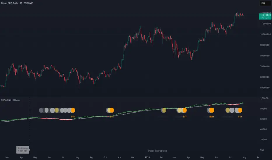
BUY in HASH RibbonsHash Ribbons Indicator (BUY Signal)
A TradingView Pine Script v6 implementation for identifying Bitcoin miner capitulation (“Springs”) and recovery phases based on hash rate data. It marks potential low-risk buying opportunities by tracking short- and long-term moving averages of the network hash rate.
⸻
Key Features
• Hash Rate SMAs
• Short-term SMA (default: 30 days)
• Long-term SMA (default: 60 days)
• Phase Markers
• Gray circle: Short SMA crosses below long SMA (start of capitulation)
• White circles: Ongoing capitulation, with brighter white when the short SMA turns upward
• Yellow circle: Short SMA crosses back above long SMA (end of capitulation)
• Orange circle: Buy signal once hash rate recovery aligns with bullish price momentum (10-day price SMA crosses above 20-day price SMA)
• Display Modes
• Ribbons: Plots the two SMAs as colored bands—red for capitulation, green for recovery
• Oscillator: Shows the percentage difference between SMAs as a histogram (red for negative, blue for positive)
• Optional Overlays
• Bitcoin halving dates (2012, 2016, 2020, 2024) with dashed lines and labels
• Raw hash rate data in EH/s
• Alerts
• Configurable alerts for capitulation start, recovery, and buy signals
⸻
How It Works
1. Data Source: Fetches daily hash rate values from a selected provider (e.g., IntoTheBlock, Quandl).
2. Capitulation Detection: When the 30-day SMA falls below the 60-day SMA, miners are likely capitulating.
3. Recovery Identification: A rising 30-day SMA during capitulation signals miner recovery.
4. Buy Signal: Confirmed when the hash rate recovery coincides with a bullish shift in price momentum (10-day price SMA > 20-day price SMA).
⸻
Inputs
Hash Rate Short SMA: 30 days
Hash Rate Long SMA: 60 days
Plot Signals: On
Plot Halvings: Off
Plot Raw Hash Rate: Off
⸻
Considerations
• Timeframe: Best applied on daily charts to capture meaningful miner behavior.
• Data Reliability: Ensure the chosen hash rate source provides consistent, gap-free data.
• Risk Management: Use alongside other technical indicators (e.g., RSI, MACD) and fundamental analysis.
• Backtesting: Evaluate performance over different market cycles before live deployment.
Bear Market Probability Model# Bear Market Probability Model: A Multi-Factor Risk Assessment Framework
The Bear Market Probability Model represents a comprehensive quantitative framework for assessing systemic market risk through the integration of 13 distinct risk factors across four analytical categories: macroeconomic indicators, technical analysis factors, market sentiment measures, and market breadth metrics. This indicator synthesizes established financial research methodologies to provide real-time probabilistic assessments of impending bear market conditions, offering institutional-grade risk management capabilities to retail and professional traders alike.
## Theoretical Foundation
### Historical Context of Bear Market Prediction
Bear market prediction has been a central focus of financial research since the seminal work of Dow (1901) and the subsequent development of technical analysis theory. The challenge of predicting market downturns gained renewed academic attention following the market crashes of 1929, 1987, 2000, and 2008, leading to the development of sophisticated multi-factor models.
Fama and French (1989) demonstrated that certain financial variables possess predictive power for stock returns, particularly during market stress periods. Their three-factor model laid the groundwork for multi-dimensional risk assessment, which this indicator extends through the incorporation of real-time market microstructure data.
### Methodological Framework
The model employs a weighted composite scoring methodology based on the theoretical framework established by Campbell and Shiller (1998) for market valuation assessment, extended through the incorporation of high-frequency sentiment and technical indicators as proposed by Baker and Wurgler (2006) in their seminal work on investor sentiment.
The mathematical foundation follows the general form:
Bear Market Probability = Σ(Wi × Ci) / ΣWi × 100
Where:
- Wi = Category weight (i = 1,2,3,4)
- Ci = Normalized category score
- Categories: Macroeconomic, Technical, Sentiment, Breadth
## Component Analysis
### 1. Macroeconomic Risk Factors
#### Yield Curve Analysis
The inclusion of yield curve inversion as a primary predictor follows extensive research by Estrella and Mishkin (1998), who demonstrated that the term spread between 3-month and 10-year Treasury securities has historically preceded all major recessions since 1969. The model incorporates both the 2Y-10Y and 3M-10Y spreads to capture different aspects of monetary policy expectations.
Implementation:
- 2Y-10Y Spread: Captures market expectations of monetary policy trajectory
- 3M-10Y Spread: Traditional recession predictor with 12-18 month lead time
Scientific Basis: Harvey (1988) and subsequent research by Ang, Piazzesi, and Wei (2006) established the theoretical foundation linking yield curve inversions to economic contractions through the expectations hypothesis of the term structure.
#### Credit Risk Premium Assessment
High-yield credit spreads serve as a real-time gauge of systemic risk, following the methodology established by Gilchrist and Zakrajšek (2012) in their excess bond premium research. The model incorporates the ICE BofA High Yield Master II Option-Adjusted Spread as a proxy for credit market stress.
Threshold Calibration:
- Normal conditions: < 350 basis points
- Elevated risk: 350-500 basis points
- Severe stress: > 500 basis points
#### Currency and Commodity Stress Indicators
The US Dollar Index (DXY) momentum serves as a risk-off indicator, while the Gold-to-Oil ratio captures commodity market stress dynamics. This approach follows the methodology of Akram (2009) and Beckmann, Berger, and Czudaj (2015) in analyzing commodity-currency relationships during market stress.
### 2. Technical Analysis Factors
#### Multi-Timeframe Moving Average Analysis
The technical component incorporates the well-established moving average convergence methodology, drawing from the work of Brock, Lakonishok, and LeBaron (1992), who provided empirical evidence for the profitability of technical trading rules.
Implementation:
- Price relative to 50-day and 200-day simple moving averages
- Moving average convergence/divergence analysis
- Multi-timeframe MACD assessment (daily and weekly)
#### Momentum and Volatility Analysis
The model integrates Relative Strength Index (RSI) analysis following Wilder's (1978) original methodology, combined with maximum drawdown analysis based on the work of Magdon-Ismail and Atiya (2004) on optimal drawdown measurement.
### 3. Market Sentiment Factors
#### Volatility Index Analysis
The VIX component follows the established research of Whaley (2009) and subsequent work by Bekaert and Hoerova (2014) on VIX as a predictor of market stress. The model incorporates both absolute VIX levels and relative VIX spikes compared to the 20-day moving average.
Calibration:
- Low volatility: VIX < 20
- Elevated concern: VIX 20-25
- High fear: VIX > 25
- Panic conditions: VIX > 30
#### Put-Call Ratio Analysis
Options flow analysis through put-call ratios provides insight into sophisticated investor positioning, following the methodology established by Pan and Poteshman (2006) in their analysis of informed trading in options markets.
### 4. Market Breadth Factors
#### Advance-Decline Analysis
Market breadth assessment follows the classic work of Fosback (1976) and subsequent research by Brown and Cliff (2004) on market breadth as a predictor of future returns.
Components:
- Daily advance-decline ratio
- Advance-decline line momentum
- McClellan Oscillator (Ema19 - Ema39 of A-D difference)
#### New Highs-New Lows Analysis
The new highs-new lows ratio serves as a market leadership indicator, based on the research of Zweig (1986) and validated in academic literature by Zarowin (1990).
## Dynamic Threshold Methodology
The model incorporates adaptive thresholds based on rolling volatility and trend analysis, following the methodology established by Pagan and Sossounov (2003) for business cycle dating. This approach allows the model to adjust sensitivity based on prevailing market conditions.
Dynamic Threshold Calculation:
- Warning Level: Base threshold ± (Volatility × 1.0)
- Danger Level: Base threshold ± (Volatility × 1.5)
- Bounds: ±10-20 points from base threshold
## Professional Implementation
### Institutional Usage Patterns
Professional risk managers typically employ multi-factor bear market models in several contexts:
#### 1. Portfolio Risk Management
- Tactical Asset Allocation: Reducing equity exposure when probability exceeds 60-70%
- Hedging Strategies: Implementing protective puts or VIX calls when warning thresholds are breached
- Sector Rotation: Shifting from growth to defensive sectors during elevated risk periods
#### 2. Risk Budgeting
- Value-at-Risk Adjustment: Incorporating bear market probability into VaR calculations
- Stress Testing: Using probability levels to calibrate stress test scenarios
- Capital Requirements: Adjusting regulatory capital based on systemic risk assessment
#### 3. Client Communication
- Risk Reporting: Quantifying market risk for client presentations
- Investment Committee Decisions: Providing objective risk metrics for strategic decisions
- Performance Attribution: Explaining defensive positioning during market stress
### Implementation Framework
Professional traders typically implement such models through:
#### Signal Hierarchy:
1. Probability < 30%: Normal risk positioning
2. Probability 30-50%: Increased hedging, reduced leverage
3. Probability 50-70%: Defensive positioning, cash building
4. Probability > 70%: Maximum defensive posture, short exposure consideration
#### Risk Management Integration:
- Position Sizing: Inverse relationship between probability and position size
- Stop-Loss Adjustment: Tighter stops during elevated risk periods
- Correlation Monitoring: Increased attention to cross-asset correlations
## Strengths and Advantages
### 1. Comprehensive Coverage
The model's primary strength lies in its multi-dimensional approach, avoiding the single-factor bias that has historically plagued market timing models. By incorporating macroeconomic, technical, sentiment, and breadth factors, the model provides robust risk assessment across different market regimes.
### 2. Dynamic Adaptability
The adaptive threshold mechanism allows the model to adjust sensitivity based on prevailing volatility conditions, reducing false signals during low-volatility periods and maintaining sensitivity during high-volatility regimes.
### 3. Real-Time Processing
Unlike traditional academic models that rely on monthly or quarterly data, this indicator processes daily market data, providing timely risk assessment for active portfolio management.
### 4. Transparency and Interpretability
The component-based structure allows users to understand which factors are driving risk assessment, enabling informed decision-making about model signals.
### 5. Historical Validation
Each component has been validated in academic literature, providing theoretical foundation for the model's predictive power.
## Limitations and Weaknesses
### 1. Data Dependencies
The model's effectiveness depends heavily on the availability and quality of real-time economic data. Federal Reserve Economic Data (FRED) updates may have lags that could impact model responsiveness during rapidly evolving market conditions.
### 2. Regime Change Sensitivity
Like most quantitative models, the indicator may struggle during unprecedented market conditions or structural regime changes where historical relationships break down (Taleb, 2007).
### 3. False Signal Risk
Multi-factor models inherently face the challenge of balancing sensitivity with specificity. The model may generate false positive signals during normal market volatility periods.
### 4. Currency and Geographic Bias
The model focuses primarily on US market indicators, potentially limiting its effectiveness for global portfolio management or non-USD denominated assets.
### 5. Correlation Breakdown
During extreme market stress, correlations between risk factors may increase dramatically, reducing the model's diversification benefits (Forbes and Rigobon, 2002).
## References
Akram, Q. F. (2009). Commodity prices, interest rates and the dollar. Energy Economics, 31(6), 838-851.
Ang, A., Piazzesi, M., & Wei, M. (2006). What does the yield curve tell us about GDP growth? Journal of Econometrics, 131(1-2), 359-403.
Baker, M., & Wurgler, J. (2006). Investor sentiment and the cross‐section of stock returns. The Journal of Finance, 61(4), 1645-1680.
Baker, S. R., Bloom, N., & Davis, S. J. (2016). Measuring economic policy uncertainty. The Quarterly Journal of Economics, 131(4), 1593-1636.
Barber, B. M., & Odean, T. (2001). Boys will be boys: Gender, overconfidence, and common stock investment. The Quarterly Journal of Economics, 116(1), 261-292.
Beckmann, J., Berger, T., & Czudaj, R. (2015). Does gold act as a hedge or a safe haven for stocks? A smooth transition approach. Economic Modelling, 48, 16-24.
Bekaert, G., & Hoerova, M. (2014). The VIX, the variance premium and stock market volatility. Journal of Econometrics, 183(2), 181-192.
Brock, W., Lakonishok, J., & LeBaron, B. (1992). Simple technical trading rules and the stochastic properties of stock returns. The Journal of Finance, 47(5), 1731-1764.
Brown, G. W., & Cliff, M. T. (2004). Investor sentiment and the near-term stock market. Journal of Empirical Finance, 11(1), 1-27.
Campbell, J. Y., & Shiller, R. J. (1998). Valuation ratios and the long-run stock market outlook. The Journal of Portfolio Management, 24(2), 11-26.
Dow, C. H. (1901). Scientific stock speculation. The Magazine of Wall Street.
Estrella, A., & Mishkin, F. S. (1998). Predicting US recessions: Financial variables as leading indicators. Review of Economics and Statistics, 80(1), 45-61.
Fama, E. F., & French, K. R. (1989). Business conditions and expected returns on stocks and bonds. Journal of Financial Economics, 25(1), 23-49.
Forbes, K. J., & Rigobon, R. (2002). No contagion, only interdependence: measuring stock market comovements. The Journal of Finance, 57(5), 2223-2261.
Fosback, N. G. (1976). Stock market logic: A sophisticated approach to profits on Wall Street. The Institute for Econometric Research.
Gilchrist, S., & Zakrajšek, E. (2012). Credit spreads and business cycle fluctuations. American Economic Review, 102(4), 1692-1720.
Harvey, C. R. (1988). The real term structure and consumption growth. Journal of Financial Economics, 22(2), 305-333.
Kahneman, D., & Tversky, A. (1979). Prospect theory: An analysis of decision under risk. Econometrica, 47(2), 263-291.
Magdon-Ismail, M., & Atiya, A. F. (2004). Maximum drawdown. Risk, 17(10), 99-102.
Nickerson, R. S. (1998). Confirmation bias: A ubiquitous phenomenon in many guises. Review of General Psychology, 2(2), 175-220.
Pagan, A. R., & Sossounov, K. A. (2003). A simple framework for analysing bull and bear markets. Journal of Applied Econometrics, 18(1), 23-46.
Pan, J., & Poteshman, A. M. (2006). The information in option volume for future stock prices. The Review of Financial Studies, 19(3), 871-908.
Taleb, N. N. (2007). The black swan: The impact of the highly improbable. Random House.
Whaley, R. E. (2009). Understanding the VIX. The Journal of Portfolio Management, 35(3), 98-105.
Wilder, J. W. (1978). New concepts in technical trading systems. Trend Research.
Zarowin, P. (1990). Size, seasonality, and stock market overreaction. Journal of Financial and Quantitative Analysis, 25(1), 113-125.
Zweig, M. E. (1986). Winning on Wall Street. Warner Books.

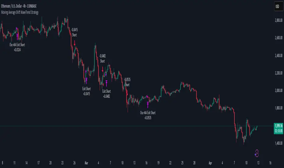
Moving Average Shift WaveTrend StrategyMoving Average Shift WaveTrend Strategy
🧭 Overview
The Moving Average Shift WaveTrend Strategy is a trend-following and momentum-based trading system designed to be overlayed on TradingView charts. It executes trades based on the confluence of multiple technical conditions—volatility, session timing, trend direction, and oscillator momentum—to deliver logical and systematic trade entries and exits.
🎯 Strategy Objectives
Enter trades aligned with the prevailing long-term trend
Exit trades on confirmed momentum reversals
Avoid false signals using session timing and volatility filters
Apply structured risk management with automatic TP, SL, and trailing stops
⚙️ Key Features
Selectable MA types: SMA, EMA, SMMA (RMA), WMA, VWMA
Dual-filter logic using a custom oscillator and moving averages
Session and volatility filters to eliminate low-quality setups
Trailing stop, configurable Take Profit / Stop Loss logic
“In-wave flag” prevents overtrading within the same trend wave
Visual clarity with color-shifting candles and entry/exit markers
📈 Trading Rules
✅ Long Entry Conditions:
Price is above the selected MA
Oscillator is positive and rising
200-period EMA indicates an uptrend
ATR exceeds its median value (sufficient volatility)
Entry occurs between 09:00–17:00 (exchange time)
Not currently in an active wave
🔻 Short Entry Conditions:
Price is below the selected MA
Oscillator is negative and falling
200-period EMA indicates a downtrend
All other long-entry conditions are inverted
❌ Exit Conditions:
Take Profit or Stop Loss is hit
Opposing signals from oscillator and MA
Trailing stop is triggered
🛡️ Risk Management Parameters
Pair: ETH/USD
Timeframe: 4H
Starting Capital: $3,000
Commission: 0.02%
Slippage: 2 pips
Risk per Trade: 2% of account equity (adjustable)
Total Trades: 224
Backtest Period: May 24, 2016 — April 7, 2025
Note: Risk parameters are fully customizable to suit your trading style and broker conditions.
🔧 Trading Parameters & Filters
Time Filter: Trades allowed only between 09:00–17:00 (exchange time)
Volatility Filter: ATR must be above its median value
Trend Filter: Long-term 200-period EMA
📊 Technical Settings
Moving Average
Type: SMA
Length: 40
Source: hl2
Oscillator
Length: 15
Threshold: 0.5
Risk Management
Take Profit: 1.5%
Stop Loss: 1.0%
Trailing Stop: 1.0%
👁️ Visual Support
MA and oscillator color changes indicate directional bias
Clear chart markers show entry and exit points
Trailing stops and risk controls are transparently managed
🚀 Strategy Improvements & Uniqueness
In-wave flag avoids repeated entries within the same trend phase
Filtering based on time, volatility, and trend ensures higher-quality trades
Dynamic high/low tracking allows precise trailing stop placement
Fully rule-based execution reduces emotional decision-making
💡 Inspirations & Attribution
This strategy is inspired by the excellent concept from:
ChartPrime – “Moving Average Shift”
It expands on the original idea with advanced trade filters and trailing logic.
Source reference:
📌 Summary
The Moving Average Shift WaveTrend Strategy offers a rule-based, reliable approach to trend trading. By combining trend and momentum filters with robust risk controls, it provides a consistent framework suitable for various market conditions and trading styles.
⚠️ Disclaimer
This script is for educational purposes only. Trading involves risk. Always use proper backtesting and risk evaluation before applying in live markets.
Bitcoin Halving DatesBitcoin Halving Dates Indicator
This custom indicator automatically marks Bitcoin's key halving events by drawing vertical lines on your chart. It highlights the historical halving dates (2012, 2016, 2020) and includes an estimated date for the upcoming halving in 2024, making it easy to visualize significant supply events that can influence market trends.
Features:
Automated Markings: Displays vertical lines on the first bar of each halving day.
Customizable: Easily adjust halving dates and styling options to suit your analysis.
Built for Traders: Enhance your technical analysis by keeping track of pivotal market events.
Use this indicator to gain a visual edge by integrating critical Bitcoin halving events into your trading strategy. Happy Trading!

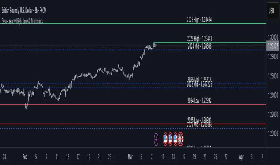
Essa - Yearly High, Low & MidYearly High, Low & Midpoint Indicator
This TradingView indicator helps traders track key yearly price levels by plotting the high, low, and midpoint values for each year within a user-specified range.
Features & Functionality:
Automatic Yearly Calculation: Determines the highest and lowest price for each year and computes the midpoint as their average.
Clear & Customisable Visuals:
The Yearly High is plotted as a solid green line.
The Yearly Low appears as a solid red line.
The Midpoint is displayed as a blue dashed line for easy distinction
Detailed Labels:
Each level is labeled at the far right of the chart, showing the year, level type (High, Low, or Mid), and price (e.g., 2016 High - 1.20000).
Labels are right-aligned in white, ensuring clear visibility against any background.
This indicator is perfect for traders who rely on long-term technical analysis, providing a quick and structured way to visualise significant yearly price levels.
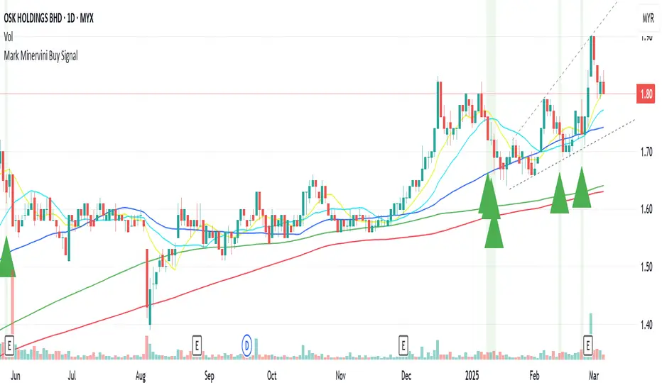
Mark Minervini Buy Signal# Mark Minervini Buy Signal Indicator
This indicator implements Mark Minervini's "Stage 2 Uptrend" buy criteria from his SEPA (Specific Entry Point Analysis) methodology as described in his books "Trade Like a Stock Market Wizard" and "Think & Trade Like a Champion". The script identifies potential buy setups based on Minervini's technical criteria for stocks showing strong momentum characteristics.
## How It Works
The indicator evaluates various technical conditions to identify stocks in a Stage 2 uptrend according to Minervini's methodology:
1. **Moving Average Alignment**
- 150-day MA above 200-day MA (confirming overall uptrend)
- 200-day MA trending up (compared to 20 days ago)
- 50-day MA above both 150-day and 200-day MAs (showing recent strength)
- Price above all major moving averages (50, 150, 200-day MAs)
2. **Price Relative to 52-Week Range**
- Price at least 25% above 52-week low (showing strong recovery)
- Price within 75-95% of 52-week high (room for further upside)
3. **Relative Strength**
- Stock ranks in the top 30% based on 100-day price performance
- This implements Minervini's emphasis on buying only strong performers
4. **Volume Criteria**
- Volume above its 50-day moving average (showing increasing interest)
## How to Use This Indicator
When all conditions are met, the indicator displays a green triangle below the price bar and colors the background green. These signals identify potential candidates for further analysis. According to Minervini's methodology, you should:
1. Use this as a screening tool to identify potential candidates
2. Perform additional chart analysis to identify specific entry points
3. Look for decreased volatility and proper bases or consolidation patterns
4. Consider broader market conditions and sector strength before entering
## Sources and Credit
This indicator is based on Mark Minervini's trading methodology as outlined in:
1. Minervini, Mark. "Trade Like a Stock Market Wizard: How to Achieve Super Performance in Stocks in Any Market" (2013)
2. Minervini, Mark. "Think & Trade Like a Champion: The Secrets, Rules & Blunt Truths of a Stock Market Wizard" (2016)
3. Minervini, Mark. "Mindset Secrets for Winning: How to Bring Personal Power to Everything You Do" (2019)
4. Interviews and workshops where Minervini has described his SEPA methodology
The specific criteria implemented are derived from Minervini's "Stage Analysis" framework, particularly focusing on Stage 2 uptrends which he considers optimal for buying opportunities.
## Disclaimer
This indicator is provided for informational purposes only. It attempts to reproduce Minervini's published criteria but should be used as part of a complete trading strategy with proper risk management. Minervini's complete methodology includes additional subjective elements that cannot be fully automated.
BTC Seasonality Strategy (Weekly)This strategy identifies potential weekend opportunities in Bitcoin (BTC) markets by leveraging the concept of seasonality, entering a position at a predefined time and day, and exiting at a specified time and day.
Key Features
Customizable Time and Day Selection:
Users can select the entry and exit days and corresponding times (in EST).
Directional Flexibility:
The strategy allows traders to choose between long or short positions.
TradingView Compliance:
The script adheres to TradingView's house rules, avoids overly complex conditions, and provides clear user-configurable inputs.
How It Works
The script determines the current weekday and hour in EST, converting TradingView's UTC time for accurate comparisons.
If the current day and hour match the selected entry conditions, a trade (long or short) is opened.
The position is closed when the current day and hour match the specified exit conditions.
Theoretical Basis
Market Seasonality:
The concept of seasonality in financial markets refers to predictable patterns based on time, such as weekends or specific days of the week. Studies have shown that cryptocurrency markets exhibit unique trading behaviors during weekends due to reduced institutional activity and higher retail participation behavioral Biases**:
Retail traders often dominate weekend markets, potentially causing predictable inefficiencies .
Reverences**
Baur, D. G., Hong, K., & Lee, A. D. (2018). Bitcoin: Medium of exchange or speculative assets? Journal of International Financial Markets, Institutions and Money, 54, 177–189.
Urquhart, A. (2016). The inefficiency of Bitcoin. Economics Letters, 148, 80–82.

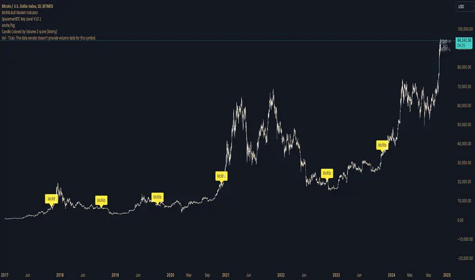
McRib Bull Market Indicator# McRib Bull Market Indicator
## Overview
The McRib Bull Market Indicator is a unique technical analysis tool that marks McDonald's McRib sandwich release dates on your trading charts. While seemingly unconventional, this indicator serves as a fascinating historical reference point for market analysis, particularly for studying periods of market expansion.
## Key Features
- Visual yellow labels marking verified McRib release dates from 2012 to 2024
- Clean, unobtrusive design that overlays on any chart timeframe
- Covers both U.S. and international releases (including UK and Australia)
## Historical Reference Points
The indicator includes release dates from:
- December 2012
- October-December 2014
- January 2015
- October 2016
- November 2017
- October 2018
- October 2019
- December 2020
- October 2022
- November 2023
- December 2024
## Usage Guide
1. Add the indicator to any chart by searching for "McRib Bull Market Indicator"
2. The indicator will automatically display yellow labels above price candles on McRib release dates
3. Use these reference points to:
- Analyze market conditions during McRib releases
- Study potential correlations between releases and market movements
- Compare market behavior across different McRib release periods
- Identify any patterns in market expansion phases coinciding with releases
## Trading Application
While initially created as a novelty indicator, it can be used to:
- Mark specific historical points of reference for broader market analysis
- Study potential market psychology around major promotional events
- Compare seasonal market patterns with recurring release dates
- Analyze market expansion phases that coincide with releases
Remember: While this indicator provides interesting historical reference points, it should be used as part of a comprehensive trading strategy rather than as a standalone trading signal.
Pulse DPO: Major Cycle Tops and Bottoms█ OVERVIEW
Pulse DPO is an oscillator designed to highlight Major Cycle Tops and Bottoms .
It works on any market driven by cycles. It operates by removing the short-term noise from the price action and focuses on the market's cyclical nature.
This indicator uses a Normalized version of the Detrended Price Oscillator (DPO) on a 0-100 scale, making it easier to identify major tops and bottoms.
Credit: The DPO was first developed by William Blau in 1991.
█ HOW TO READ IT
Pulse DPO oscillates in the range between 0 and 100. A value in the upper section signals an OverBought (OB) condition, while a value in the lower section signals an OverSold (OS) condition.
Generally, the triggering of OB and OS conditions don't necessarily translate into swing tops and bottoms, but rather suggest caution on approaching a market that might be overextended.
Nevertheless, this indicator has been customized to trigger the signal only during remarkable top and bottom events.
I suggest using it on the Daily Time Frame , but you're free to experiment with this indicator on other time frames.
The indicator has Built-in Alerts to signal the crossing of the Thresholds. Please don't act on an isolated signal, but rather integrate it to work in conjunction with the indicators present in your Trading Plan.
█ OB SIGNAL ON: ENTERING OVERBOUGHT CONDITION
When Pulse DPO crosses Above the Top Threshold it Triggers ON the OB signal. At this point the oscillator line shifts to OB color.
When Pulse DPO enters the OB Zone, please beware! In this Area the Major Players usually become Active Sellers to the Public. While the OB signal is On, it might be wise to Consider Selling a portion or the whole Long Position.
Please note that even though this indicator aims to focus on major tops and bottoms, a strong trending market might trigger the OB signal and stay with it for a long time. That's especially true on young markets and on bubble-mode markets.
█ OB SIGNAL OFF: EXITING OVERBOUGHT CONDITION
When Pulse DPO crosses Below the Top Threshold it Triggers OFF the OB signal. At this point the oscillator line shifts to its normal color.
When Pulse DPO exits the OB Zone, please beware because a Major Top might just have occurred. In this Area the Major Players usually become Aggressive Sellers. They might wind up any remaining Long Positions and Open new Short Positions.
This might be a good area to Open Shorts or to Close/Reverse any remaining Long Position. Whatever you choose to do, it's usually best to act quickly because the market is prone to enter into panic mode.
█ OS SIGNAL ON: ENTERING OVERSOLD CONDITION
When Pulse DPO crosses Below the Bottom Threshold it Triggers ON the OS signal. At this point the oscillator line shifts to OS color.
When Pulse DPO enters the OS Zone, please beware because in this Area the Major Players usually become Active Buyers accumulating Long Positions from the desperate Public.
While the OS signal is On, it might be wise to Consider becoming a Buyer or to implement a Dollar-Cost Averaging (DCA) Strategy to build a Long Position towards the next Cycle. In contrast to the tops, the OS state usually takes longer to resolve a major bottom.
█ OS SIGNAL OFF: EXITING OVERSOLD CONDITION
When Pulse DPO crosses Above the Bottom Threshold it Triggers OFF the OS signal. At this point the oscillator line shifts to its normal color.
When Pulse DPO exits the OS Zone, please beware because a Major Bottom might already be in place. In this Area the Major Players become Aggresive Buyers. They might wind up any remaining Short Positions and Open new Long Positions.
This might be a good area to Open Longs or to Close/Reverse any remaining Short Positions.
█ WHY WOULD YOU BE INTERESTED IN THIS INDICATOR?
This indicator is built over a solid foundation capable of signaling Major Cycle Tops and Bottoms across many markets. Let's see some examples:
Early Bitcoin Years: From 0 to 1242
This chart is in logarithmic mode in order to properly display various exponential cycles. Pulse DPO is properly signaling the major early highs from 9-Jun-2011 at 31.50, to the next one on 9-Apr-2013 at 240 and the epic top from 29-Nov-2013 at 1242.
Due to the massive price movements, the OB condition stays pinned during most of the exponential price action. But as you can see, the OB condition quickly vanishes once the Cycle Top has been reached. As the market matures, the OB condition becomes more exceptional and triggers much closer from the Cycle Top.
With regards to Cycle Bottoms, the early bottom of 2 after having peaked at 31.50 doesn’t get captured by the indicator. That is the only cycle bottom that escapes the Pulse DPO when the bottom threshold is set at a value of 5. In that event, the oscillator low reached 6.95.
Bitcoin Adoption Spreading: From 257 to 73k
This chart is in logarithmic mode in order to properly display various exponential cycles. Pulse DPO is properly signaling all the major highs from 17-Dec-2017 at 19k, to the next one on 14-Apr-2021 at 64k and the most recent top from 9-Nov-2021 at 68k.
During the massive run of 2017, the OB condition still stayed triggered for a few weeks on each swing top. But on the next cycles it started to signal only for a few days before each swing top actually happened. The OB condition during the last cycle top triggered only for 3 days. Therefore the signal grows in focus as the market matures.
At the time of publishing this indicator, Bitcoin printed a new All Time High (ATH) on 13-Mar-2024 at 73k. That run didn’t trigger the OB condition. Therefore, if the indicator is correct the Bitcoin market still has some way to grow during the next months.
With regards to Cycle Bottoms, the bottom of 3k after having peaked at19k got captured within the wide OS zone. The bottom of 15k after having peaked at 68k got captured too within the OS accumulation area.
Gold
Pulse DPO behaves surprisingly well on a long standing market such as Gold. Moving back to the 197x years it’s been signaling most Cycle Tops and Bottoms with precision. During the last cycle, it shows topping at 2k and bottoming at 1.6k.
The current price action is signaling OB condition in the range of 2.5k to 2.7k. Looking at past cycles, it tends to trigger on and off at multiple swing tops until reaching the final cycle top. Therefore this might indicate the first wave within a potential gold run.
Oil
On the Oil market, we can see that most of the cycle tops and bottoms since the 80s got signaled. The only exception being the low from 2020 which didn’t trigger.
EURUSD
On Forex markets the Pulse DPO also behaves as expected. Looking back at EURUSD we can see the marketing triggering OB and OS conditions during major cycle tops and bottoms from recent times until the 80s.
S&P 500
On the S&P 500 the Pulse DPO catched the lows from 2016 and 2020. Looking at present price action, the recent ATH didn’t trigger the OB condition. Therefore, the indicator is allowing room for another leg up during the next months.
Amazon
On the Amazon chart the Pulse DPO is mirroring pretty accurately the major swings. Scrolling back to the early 2000s, this chart resembles early exponential swings in the crypto space.
Tesla
Moving onto a younger tech stock, Pulse DPO captures pretty accurately the major tops and bottoms. The chart is shown in logarithmic scale to better display the magnitude of the moves.
█ SETTINGS
This indicator is ideal for identifying major market turning points while filtering out short-term noise. You are free to adjust the parameters to align with your preferred trading style.
Parameters : This section allows you to customize any of the Parameters that shape the Oscillator.
Oscillator Length: Defines the period for calculating the Oscillator.
Offset: Shifts the oscillator calculation by a certain number of periods, which is typically half the Oscillator Length.
Lookback Period: Specifies how many bars to look back to find tops and bottoms for normalization.
Smoothing Length: Determines the length of the moving average used to smooth the oscillator.
Thresholds : This section allows you to customize the Thresholds that trigger the OB and OS conditions.
Top: Defines the value of the Top Threshold.
Bottom: Defines the value of the Bottom Threshold.

Intellect_city - Halvings Bitcoin CycleWhat is halving?
The halving timer shows when the next Bitcoin halving will occur, as well as the dates of past halvings. This event occurs every 210,000 blocks, which is approximately every 4 years. Halving reduces the emission reward by half. The original Bitcoin reward was 50 BTC per block found.
Why is halving necessary?
Halving allows you to maintain an algorithmically specified emission level. Anyone can verify that no more than 21 million bitcoins can be issued using this algorithm. Moreover, everyone can see how much was issued earlier, at what speed the emission is happening now, and how many bitcoins remain to be mined in the future. Even a sharp increase or decrease in mining capacity will not significantly affect this process. In this case, during the next difficulty recalculation, which occurs every 2014 blocks, the mining difficulty will be recalculated so that blocks are still found approximately once every ten minutes.
How does halving work in Bitcoin blocks?
The miner who collects the block adds a so-called coinbase transaction. This transaction has no entry, only exit with the receipt of emission coins to your address. If the miner's block wins, then the entire network will consider these coins to have been obtained through legitimate means. The maximum reward size is determined by the algorithm; the miner can specify the maximum reward size for the current period or less. If he puts the reward higher than possible, the network will reject such a block and the miner will not receive anything. After each halving, miners have to halve the reward they assign to themselves, otherwise their blocks will be rejected and will not make it to the main branch of the blockchain.
The impact of halving on the price of Bitcoin
It is believed that with constant demand, a halving of supply should double the value of the asset. In practice, the market knows when the halving will occur and prepares for this event in advance. Typically, the Bitcoin rate begins to rise about six months before the halving, and during the halving itself it does not change much. On average for past periods, the upper peak of the rate can be observed more than a year after the halving. It is almost impossible to predict future periods because, in addition to the reduction in emissions, many other factors influence the exchange rate. For example, major hacks or bankruptcies of crypto companies, the situation on the stock market, manipulation of “whales,” or changes in legislative regulation.
---------------------------------------------
Table - Past and future Bitcoin halvings:
---------------------------------------------
Date: Number of blocks: Award:
0 - 03-01-2009 - 0 block - 50 BTC
1 - 28-11-2012 - 210000 block - 25 BTC
2 - 09-07-2016 - 420000 block - 12.5 BTC
3 - 11-05-2020 - 630000 block - 6.25 BTC
4 - 20-04-2024 - 840000 block - 3.125 BTC
5 - 24-03-2028 - 1050000 block - 1.5625 BTC
6 - 26-02-2032 - 1260000 block - 0.78125 BTC
7 - 30-01-2036 - 1470000 block - 0.390625 BTC
8 - 03-01-2040 - 1680000 block - 0.1953125 BTC
9 - 07-12-2043 - 1890000 block - 0.09765625 BTC
10 - 10-11-2047 - 2100000 block - 0.04882813 BTC
11 - 14-10-2051 - 2310000 block - 0.02441406 BTC
12 - 17-09-2055 - 2520000 block - 0.01220703 BTC
13 - 21-08-2059 - 2730000 block - 0.00610352 BTC
14 - 25-07-2063 - 2940000 block - 0.00305176 BTC
15 - 28-06-2067 - 3150000 block - 0.00152588 BTC
16 - 01-06-2071 - 3360000 block - 0.00076294 BTC
17 - 05-05-2075 - 3570000 block - 0.00038147 BTC
18 - 08-04-2079 - 3780000 block - 0.00019073 BTC
19 - 12-03-2083 - 3990000 block - 0.00009537 BTC
20 - 13-02-2087 - 4200000 block - 0.00004768 BTC
21 - 17-01-2091 - 4410000 block - 0.00002384 BTC
22 - 21-12-2094 - 4620000 block - 0.00001192 BTC
23 - 24-11-2098 - 4830000 block - 0.00000596 BTC
24 - 29-10-2102 - 5040000 block - 0.00000298 BTC
25 - 02-10-2106 - 5250000 block - 0.00000149 BTC
26 - 05-09-2110 - 5460000 block - 0.00000075 BTC
27 - 09-08-2114 - 5670000 block - 0.00000037 BTC
28 - 13-07-2118 - 5880000 block - 0.00000019 BTC
29 - 16-06-2122 - 6090000 block - 0.00000009 BTC
30 - 20-05-2126 - 6300000 block - 0.00000005 BTC
31 - 23-04-2130 - 6510000 block - 0.00000002 BTC
32 - 27-03-2134 - 6720000 block - 0.00000001 BTC
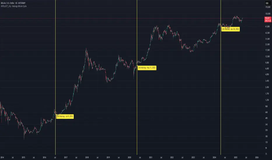
[Excalibur] Ehlers AutoCorrelation Periodogram ModifiedKeep your coins folks, I don't need them, don't want them. If you wish be generous, I do hope that charitable peoples worldwide with surplus food stocks may consider stocking local food banks before stuffing monetary bank vaults, for the crusade of remedying the needs of less than fortunate children, parents, elderly, homeless veterans, and everyone else who deserves nutritional sustenance for the soul.
DEDICATION:
This script is dedicated to the memory of Nikolai Dmitriyevich Kondratiev (Никола́й Дми́триевич Кондра́тьев) as tribute for being a pioneering economist and statistician, paving the way for modern econometrics by advocation of rigorous and empirical methodologies. One of his most substantial contributions to the study of business cycle theory include a revolutionary hypothesis recognizing the existence of dynamic cycle-like phenomenon inherent to economies that are characterized by distinct phases of expansion, stagnation, recession and recovery, what we now know as "Kondratiev Waves" (K-waves). Kondratiev was one of the first economists to recognize the vital significance of applying quantitative analysis on empirical data to evaluate economic dynamics by means of statistical methods. His understanding was that conceptual models alone were insufficient to adequately interpret real-world economic conditions, and that sophisticated analysis was necessary to better comprehend the nature of trending/cycling economic behaviors. Additionally, he recognized prosperous economic cycles were predominantly driven by a combination of technological innovations and infrastructure investments that resulted in profound implications for economic growth and development.
I will mention this... nation's economies MUST be supported and defended to continuously evolve incrementally in order to flourish in perpetuity OR suffer through eras with lasting ramifications of societal stagnation and implosion.
Analogous to the realm of economics, aperiodic cycles/frequencies, both enduring and ephemeral, do exist in all facets of life, every second of every day. To name a few that any blind man can naturally see are: heartbeat (cardiac cycles), respiration rates, circadian rhythms of sleep, powerful magnetic solar cycles, seasonal cycles, lunar cycles, weather patterns, vegetative growth cycles, and ocean waves. Do not pretend for one second that these basic aforementioned examples do not affect business cycle fluctuations in minuscule and monumental ways hour to hour, day to day, season to season, year to year, and decade to decade in every nation on the planet. Kondratiev's original seminal theories in macroeconomics from nearly a century ago have proven remarkably prescient with many of his antiquated elementary observations/notions/hypotheses in macroeconomics being scholastically studied and topically researched further. Therefore, I am compelled to honor and recognize his statistical insight and foresight.
If only.. Kondratiev could hold a pocket sized computer in the cup of both hands bearing the TradingView logo and platform services, I truly believe he would be amazed in marvelous delight with a GARGANTUAN smile on his face.
INTRODUCTION:
Firstly, this is NOT technically speaking an indicator like most others. I would describe it as an advanced cycle period detector to obtain market data spectral estimates with low latency and moderate frequency resolution. Developers can take advantage of this detector by creating scripts that utilize a "Dominant Cycle Source" input to adaptively govern algorithms. Be forewarned, I would only recommend this for advanced developers, not novice code dabbling. Although, there is some Pine wizardry introduced here for novice Pine enthusiasts to witness and learn from. AI did describe the code into one super-crunched sentence as, "a rare feat of exceptionally formatted code masterfully balancing visual clarity, precision, and complexity to provide immense educational value for both programming newcomers and expert Pine coders alike."
Understand all of the above aforementioned? Buckle up and proceed for a lengthy read of verbose complexity...
This is my enhanced and heavily modified version of autocorrelation periodogram (ACP) for Pine Script v5.0. It was originally devised by the mathemagician John Ehlers for detecting dominant cycles (frequencies) in an asset's price action. I have been sitting on code similar to this for a long time, but I decided to unleash the advanced code with my fashion. Originally Ehlers released this with multiple versions, one in a 2016 TASC article and the other in his last published 2013 book "Cycle Analytics for Traders", chapter 8. He wasn't joking about "concepts of advanced technical trading" and ACP is nowhere near to his most intimidating and ingenious calculations in code. I will say the book goes into many finer details about the original periodogram, so if you wish to delve into even more elaborate info regarding Ehlers' original ACP form AND how you may adapt algorithms, you'll have to obtain one. Note to reader, comparing Ehlers' original code to my chimeric code embracing the "Power of Pine", you will notice they have little resemblance.
What you see is a new species of autocorrelation periodogram combining Ehlers' innovation with my fascinations of what ACP could be in a Pine package. One other intention of this script's code is to pay homage to Ehlers' lifelong works. Like Kondratiev, Ehlers is also a hardcore cycle enthusiast. I intend to carry on the fire Ehlers envisioned and I believe that is literally displayed here as a pleasant "fiery" example endowed with Pine. With that said, I tried to make the code as computationally efficient as possible, without going into dozens of more crazy lines of code to speed things up even more. There's also a few creative modifications I made by making alterations to the originating formulas that I felt were improvements, one of them being lag reduction. By recently questioning every single thing I thought I knew about ACP, combined with the accumulation of my current knowledge base, this is the innovative revision I came up with. I could have improved it more but decided not to mind thrash too many TV members, maybe later...
I am now confident Pine should have adequate overhead left over to attach various indicators to the dominant cycle via input.source(). TV, I apologize in advance if in the future a server cluster combusts into a raging inferno... Coders, be fully prepared to build entire algorithms from pure raw code, because not all of the built-in Pine functions fully support dynamic periods (e.g. length=ANYTHING). Many of them do, as this was requested and granted a while ago, but some functions are just inherently finicky due to implementation combinations and MUST be emulated via raw code. I would imagine some comprehensive library or numerous authored scripts have portions of raw code for Pine built-ins some where on TV if you look diligently enough.
Notice: Unfortunately, I will not provide any integration support into member's projects at all. I have my own projects that require way too much of my day already. While I was refactoring my life (forgoing many other "important" endeavors) in the early half of 2023, I primarily focused on this code over and over in my surplus time. During that same time I was working on other innovations that are far above and beyond what this code is. I hope you understand.
The best way programmatically may be to incorporate this code into your private Pine project directly, after brutal testing of course, but that may be too challenging for many in early development. Being able to see the periodogram is also beneficial, so input sourcing may be the "better" avenue to tether portions of the dominant cycle to algorithms. Unique indication being able to utilize the dominantCycle may be advantageous when tethering this script to those algorithms. The easiest way is to manually set your indicators to what ACP recognizes as the dominant cycle, but that's actually not considered dynamic real time adaption of an indicator. Different indicators may need a proportion of the dominantCycle, say half it's value, while others may need the full value of it. That's up to you to figure that out in practice. Sourcing one or more custom indicators dynamically to one detector's dominantCycle may require code like this: `int sourceDC = int(math.max(6, math.min(49, input.source(close, "Dominant Cycle Source"))))`. Keep in mind, some algos can use a float, while algos with a for loop require an integer.
I have witnessed a few attempts by talented TV members for a Pine based autocorrelation periodogram, but not in this caliber. Trust me, coding ACP is no ordinary task to accomplish in Pine and modifying it blessed with applicable improvements is even more challenging. For over 4 years, I have been slowly improving this code here and there randomly. It is beautiful just like a real flame, but... this one can still burn you! My mind was fried to charcoal black a few times wrestling with it in the distant past. My very first attempt at translating ACP was a month long endeavor because PSv3 simply didn't have arrays back then. Anyways, this is ACP with a newer engine, I hope you enjoy it. Any TV subscriber can utilize this code as they please. If you are capable of sufficiently using it properly, please use it wisely with intended good will. That is all I beg of you.
Lastly, you now see how I have rasterized my Pine with Ehlers' swami-like tech. Yep, this whole time I have been using hline() since PSv3, not plot(). Evidently, plot() still has a deficiency limited to only 32 plots when it comes to creating intense eye candy indicators, the last I checked. The use of hline() is the optimal choice for rasterizing Ehlers styled heatmaps. This does only contain two color schemes of the many I have formerly created, but that's all that is essentially needed for this gizmo. Anything else is generally for a spectacle or seeing how brutal Pine can be color treated. The real hurdle is being able to manipulate colors dynamically with Merlin like capabilities from multiple algo results. That's the true challenging part of these heatmap contraptions to obtain multi-colored "predator vision" level indication. You now have basic hline() food for thought empowerment to wield as you can imaginatively dream in Pine projects.
PERIODOGRAM UTILITY IN REAL WORLD SCENARIOS:
This code is a testament to the abilities that have yet to be fully realized with indication advancements. Periodograms, spectrograms, and heatmaps are a powerful tool with real-world applications in various fields such as financial markets, electrical engineering, astronomy, seismology, and neuro/medical applications. For instance, among these diverse fields, it may help traders and investors identify market cycles/periodicities in financial markets, support engineers in optimizing electrical or acoustic systems, aid astronomers in understanding celestial object attributes, assist seismologists with predicting earthquake risks, help medical researchers with neurological disorder identification, and detection of asymptomatic cardiovascular clotting in the vaxxed via full body thermography. In either field of study, technologies in likeness to periodograms may very well provide us with a better sliver of analysis beyond what was ever formerly invented. Periodograms can identify dominant cycles and frequency components in data, which may provide valuable insights and possibly provide better-informed decisions. By utilizing periodograms within aspects of market analytics, individuals and organizations can potentially refrain from making blinded decisions and leverage data-driven insights instead.
PERIODOGRAM INTERPRETATION:
The periodogram renders the power spectrum of a signal, with the y-axis representing the periodicity (frequencies/wavelengths) and the x-axis representing time. The y-axis is divided into periods, with each elevation representing a period. In this periodogram, the y-axis ranges from 6 at the very bottom to 49 at the top, with intermediate values in between, all indicating the power of the corresponding frequency component by color. The higher the position occurs on the y-axis, the longer the period or lower the frequency. The x-axis of the periodogram represents time and is divided into equal intervals, with each vertical column on the axis corresponding to the time interval when the signal was measured. The most recent values/colors are on the right side.
The intensity of the colors on the periodogram indicate the power level of the corresponding frequency or period. The fire color scheme is distinctly like the heat intensity from any casual flame witnessed in a small fire from a lighter, match, or camp fire. The most intense power would be indicated by the brightest of yellow, while the lowest power would be indicated by the darkest shade of red or just black. By analyzing the pattern of colors across different periods, one may gain insights into the dominant frequency components of the signal and visually identify recurring cycles/patterns of periodicity.
SETTINGS CONFIGURATIONS BRIEFLY EXPLAINED:
Source Options: These settings allow you to choose the data source for the analysis. Using the `Source` selection, you may tether to additional data streams (e.g. close, hlcc4, hl2), which also may include samples from any other indicator. For example, this could be my "Chirped Sine Wave Generator" script found in my member profile. By using the `SineWave` selection, you may analyze a theoretical sinusoidal wave with a user-defined period, something already incorporated into the code. The `SineWave` will be displayed over top of the periodogram.
Roofing Filter Options: These inputs control the range of the passband for ACP to analyze. Ehlers had two versions of his highpass filters for his releases, so I included an option for you to see the obvious difference when performing a comparison of both. You may choose between 1st and 2nd order high-pass filters.
Spectral Controls: These settings control the core functionality of the spectral analysis results. You can adjust the autocorrelation lag, adjust the level of smoothing for Fourier coefficients, and control the contrast/behavior of the heatmap displaying the power spectra. I provided two color schemes by checking or unchecking a checkbox.
Dominant Cycle Options: These settings allow you to customize the various types of dominant cycle values. You can choose between floating-point and integer values, and select the rounding method used to derive the final dominantCycle values. Also, you may control the level of smoothing applied to the dominant cycle values.
DOMINANT CYCLE VALUE SELECTIONS:
External to the acs() function, the code takes a dominant cycle value returned from acs() and changes its numeric form based on a specified type and form chosen within the indicator settings. The dominant cycle value can be represented as an integer or a decimal number, depending on the attached algorithm's requirements. For example, FIR filters will require an integer while many IIR filters can use a float. The float forms can be either rounded, smoothed, or floored. If the resulting value is desired to be an integer, it can be rounded up/down or just be in an integer form, depending on how your algorithm may utilize it.
AUTOCORRELATION SPECTRUM FUNCTION BASICALLY EXPLAINED:
In the beginning of the acs() code, the population of caches for precalculated angular frequency factors and smoothing coefficients occur. By precalculating these factors/coefs only once and then storing them in an array, the indicator can save time and computational resources when performing subsequent calculations that require them later.
In the following code block, the "Calculate AutoCorrelations" is calculated for each period within the passband width. The calculation involves numerous summations of values extracted from the roofing filter. Finally, a correlation values array is populated with the resulting values, which are normalized correlation coefficients.
Moving on to the next block of code, labeled "Decompose Fourier Components", Fourier decomposition is performed on the autocorrelation coefficients. It iterates this time through the applicable period range of 6 to 49, calculating the real and imaginary parts of the Fourier components. Frequencies 6 to 49 are the primary focus of interest for this periodogram. Using the precalculated angular frequency factors, the resulting real and imaginary parts are then utilized to calculate the spectral Fourier components, which are stored in an array for later use.
The next section of code smooths the noise ridden Fourier components between the periods of 6 and 49 with a selected filter. This species also employs numerous SuperSmoothers to condition noisy Fourier components. One of the big differences is Ehlers' versions used basic EMAs in this section of code. I decided to add SuperSmoothers.
The final sections of the acs() code determines the peak power component for normalization and then computes the dominant cycle period from the smoothed Fourier components. It first identifies a single spectral component with the highest power value and then assigns it as the peak power. Next, it normalizes the spectral components using the peak power value as a denominator. It then calculates the average dominant cycle period from the normalized spectral components using Ehlers' "Center of Gravity" calculation. Finally, the function returns the dominant cycle period along with the normalized spectral components for later external use to plot the periodogram.
POST SCRIPT:
Concluding, I have to acknowledge a newly found analyst for assistance that I couldn't receive from anywhere else. For one, Claude doesn't know much about Pine, is unfortunately color blind, and can't even see the Pine reference, but it was able to intuitively shred my code with laser precise realizations. Not only that, formulating and reformulating my description needed crucial finesse applied to it, and I couldn't have provided what you have read here without that artificial insight. Finding the right order of words to convey the complexity of ACP and the elaborate accompanying content was a daunting task. No code in my life has ever absorbed so much time and hard fricking work, than what you witness here, an ACP gem cut pristinely. I'm unveiling my version of ACP for an empowering cause, in the hopes a future global army of code wielders will tether it to highly functional computational contraptions they might possess. Here is ACP fully blessed poetically with the "Power of Pine" in sublime code. ENJOY!
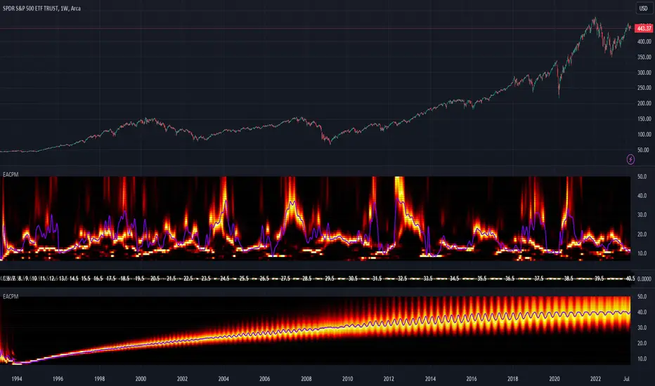
Financial Ratios Fundamental StrategyWhat are financial ratios?
Financial ratios are basic calculations using quantitative data from a company’s financial statements. They are used to get insights and important information on the company’s performance, profitability, and financial health.
Common financial ratios come from a company’s balance sheet, income statement, and cash flow statement.
Businesses use financial ratios to determine liquidity, debt concentration, growth, profitability, and market value.
The common financial ratios every business should track are
1) liquidity ratios
2) leverage ratios
3)efficiency ratio
4) profitability ratios
5) market value ratios.
Initially I had a big list of 20 different ratios for testing, but in the end I decided to stick for the strategy with these ones :
Current ratio: Current Assets / Current Liabilities
The current ratio measures how a business’s current assets, such as cash, cash equivalents, accounts receivable, and inventories, are used to settle current liabilities such as accounts payable.
Interest coverage ratio: EBIT / Interest expenses
Companies generally pay interest on corporate debt. The interest coverage ratio shows if a company’s revenue after operating expenses can cover interest liabilities.
Payables turnover ratio: Cost of Goods sold (or net credit purchases) / Average Accounts Payable
The payables turnover ratio calculates how quickly a business pays its suppliers and creditors.
Gross margin: Gross profit / Net sales
The gross margin ratio measures how much profit a business makes after the cost of goods and services compared to net sales.
With this data, I have created the long and long exit strategy:
For long, if any of the 4 listed ratios,such as current ratio or interest coverage ratio or payable turn ratio or gross margin ratio is ascending after a quarter, its a potential long entry.
For example in january the gross margin ratio is at 10% and in april is at 15%, this is an increase from a quarter to another, so it will get a long entry trigger.
The same could happen if any of the 4 listed ratios follow the ascending condition since they are all treated equally as important
For exit, if any of the 4 listed ratios are descending after a quarter, such as current ratio or interest coverage ratio or payable turn ratio or gross margin ratio is descending after a quarter, its a potential long exit.
For example in april we entered a long trade, and in july data from gross margin comes as 12% .
In this case it fell down from 15% to 12%, triggering an exit for our trade.
However there is a special case with this strategy, in order to make it more re active and make use of the compound effect:
So lets say on july 1 when the data came in, the gross margin data came descending (indicating an exit for the long trade), however at the same the interest coverage ratio came as positive, or any of the other 3 left ratios left . In that case the next day after the trade closed, it will enter a new long position and wait again until a new quarter data for the financial is being published.
Regarding the guidelines of tradingview, they recommend to have more than 100 trades.
With this type of strategy, using Daily timeframe and data from financials coming each quarter(4 times a year), we only have the financial data available since 2016, so that makes 28 quarters of data, making a maximum potential of 28 trades.
This can however be "bypassed" to check the integrity of the strategy and its edge, by taking for example multiple stocks and test them in a row, for example, appl, msft, goog, brk and so on, and you can see the correlation between them all.
At the same time I have to say that this strategy is more as an educational one since it miss a risk management and other additional filters to make it more adapted for real live trading, and instead serves as a guiding tool for those that want to make use of fundamentals in their trades
If you have any questions, please let me know !
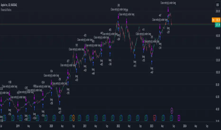
Yearly Monthly Vertical Lines [MsF]This indicator that draws vertical lines for each year and month starting from the specified date and time.
For example, starting from August 26th, 2022,
The annual vertical lines are Aug 26th, 2022, Aug 26th, 2021, Aug 26th, 2020, Aug 26th, 2019, Aug 26th, 2018, Aug 26th, 2017...
It is useful to check the action of the chart at the event of each year and month.
Caution:
Since there is a limit to the Bar-Count that can be specified in the script language, depending on the chart period setting It may not be displayed.
-------------------------
指定した日時を起点として、年、月ごとに垂直線(縦線)を描画するインジケータです。
例えば、2022/9/1を起点とした場合、
年次のラインは、2021/9/1、2020/9/1、2019/9/1、2018/9/1、2017/9/1、2016/9/1...
に描画します。
年、月ごとのイベント時のチャートの動きを確認するのに便利です。
※過去イベント時の価格変動確認の際、手作業で垂直線を引くのが面倒なため、作成しました。
<注意>
スクリプト言語で指定できるBarCntに制限がある為、チャートの期間設定によっては
表示されない場合があります。※今後改善の余地あり

[blackcat] L1 Vitali Apirine HHs & LLs StochasticsLevel 1
Background
This indicator was originally formulated by Vitali Apirine for TASC - February 2016 Traders Tips.
Function
According to Vitali Apirine, his momentum indicator–based system HHLLS (higher high lower low stochastic) can help to spot emerging trends, define correction periods, and anticipate reversals. As with many indicators, HHLLS signals can also be generated by looking for divergences and crossovers. Because the HHLLS is an oscillator, it can also be used to identify overbought & oversold levels.
Remarks
I changed EMA or SMA into hanning windowing function to reduce lag issue.
colorful area is bearish power.
colorful solid thick line is bull power.
Feedbacks are appreciated.

Ehlers Autocorrelation Periodogram [Loxx]Ehlers Autocorrelation Periodogram contains two versions of Ehlers Autocorrelation Periodogram Algorithm. This indicator is meant to supplement adaptive cycle indicators that myself and others have published on Trading View, will continue to publish on Trading View. These are fast-loading, low-overhead, streamlined, exact replicas of Ehlers' work without any other adjustments or inputs.
Versions:
- 2013, Cycle Analytics for Traders Advanced Technical Trading Concepts by John F. Ehlers
- 2016, TASC September, "Measuring Market Cycles"
Description
The Ehlers Autocorrelation study is a technical indicator used in the calculation of John F. Ehlers’s Autocorrelation Periodogram. Its main purpose is to eliminate noise from the price data, reduce effects of the “spectral dilation” phenomenon, and reveal dominant cycle periods. The spectral dilation has been discussed in several studies by John F. Ehlers; for more information on this, refer to sources in the "Further Reading" section.
As the first step, Autocorrelation uses Mr. Ehlers’s previous installment, Ehlers Roofing Filter, in order to enhance the signal-to-noise ratio and neutralize the spectral dilation. This filter is based on aerospace analog filters and when applied to market data, it attempts to only pass spectral components whose periods are between 10 and 48 bars.
Autocorrelation is then applied to the filtered data: as its name implies, this function correlates the data with itself a certain period back. As with other correlation techniques, the value of +1 would signify the perfect correlation and -1, the perfect anti-correlation.
Using values of Autocorrelation in Thermo Mode may help you reveal the cycle periods within which the data is best correlated (or anti-correlated) with itself. Those periods are displayed in the extreme colors (orange) while areas of intermediate colors mark periods of less useful cycles.
What is an adaptive cycle, and what is the Autocorrelation Periodogram Algorithm?
From his Ehlers' book mentioned above, page 135:
"Adaptive filters can have several different meanings. For example, Perry Kaufman’s adaptive moving average ( KAMA ) and Tushar Chande’s variable index dynamic average ( VIDYA ) adapt to changes in volatility . By definition, these filters are reactive to price changes, and therefore they close the barn door after the horse is gone.The adaptive filters discussed in this chapter are the familiar Stochastic , relative strength index ( RSI ), commodity channel index ( CCI ), and band-pass filter.The key parameter in each case is the look-back period used to calculate the indicator.This look-back period is commonly a fixed value. However, since the measured cycle period is changing, as we have seen in previous chapters, it makes sense to adapt these indicators to the measured cycle period. When tradable market cycles are observed, they tend to persist for a short while.Therefore, by tuning the indicators to the measure cycle period they are optimized for current conditions and can even have predictive characteristics.
The dominant cycle period is measured using the Autocorrelation Periodogram Algorithm. That dominant cycle dynamically sets the look-back period for the indicators. I employ my own streamlined computation for the indicators that provide smoother and easier to interpret outputs than traditional methods. Further, the indicator codes have been modified to remove the effects of spectral dilation.This basically creates a whole new set of indicators for your trading arsenal."
How to use this indicator
The point of the Ehlers Autocorrelation Periodogram Algorithm is to dynamically set a period between a minimum and a maximum period length. While I leave the exact explanation of the mechanic to Dr. Ehlers’s book, for all practical intents and purposes, in my opinion, the punchline of this method is to attempt to remove a massive source of overfitting from trading system creation–namely specifying a look-back period. SMA of 50 days? 100 days? 200 days? Well, theoretically, this algorithm takes that possibility of overfitting out of your hands. Simply, specify an upper and lower bound for your look-back, and it does the rest. In addition, this indicator tells you when its best to use adaptive cycle inputs for your other indicators.
Usage Example 1
Let's say you're using "Adaptive Qualitative Quantitative Estimation (QQE) ". This indicator has the option of adaptive cycle inputs. When the "Ehlers Autocorrelation Periodogram " shows a period of high correlation that adaptive cycle inputs work best during that period.
Usage Example 2
Check where the dominant cycle line lines, grab that output number and inject it into your other standard indicators for the length input.
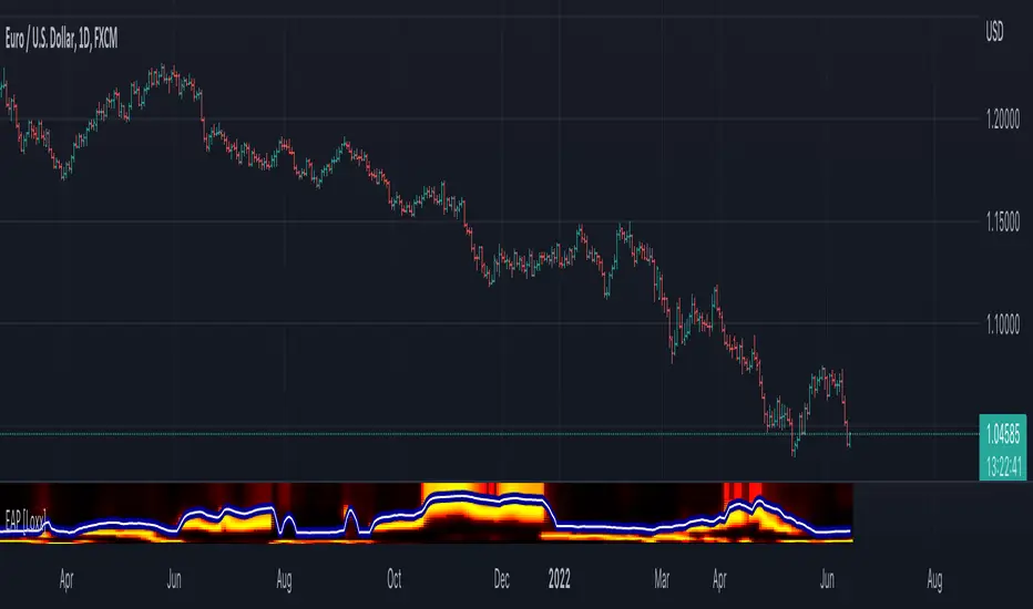
DominantCycleCollection of Dominant Cycle estimators. Length adaptation used in the Adaptive Moving Averages and the Adaptive Oscillators try to follow price movements and accelerate/decelerate accordingly (usually quite rapidly with a huge range). Cycle estimators, on the other hand, try to measure the cycle period of the current market, which does not reflect price movement or the rate of change (the rate of change may also differ depending on the cycle phase, but the cycle period itself usually changes slowly). This collection may become encyclopaedic, so if you have any working cycle estimator, drop me a line in the comments below. Suggestions are welcome. Currently included estimators are based on the work of John F. Ehlers
mamaPeriod(src, dynLow, dynHigh) MESA Adaptation - MAMA Cycle
Parameters:
src : Series to use
dynLow : Lower bound for the dynamic length
dynHigh : Upper bound for the dynamic length
Returns: Calculated period
Based on MESA Adaptive Moving Average by John F. Ehlers
Performs Hilbert Transform Homodyne Discriminator cycle measurement
Unlike MAMA Alpha function (in LengthAdaptation library), this does not compute phase rate of change
Introduced in the September 2001 issue of Stocks and Commodities
Inspired by the @everget implementation:
Inspired by the @anoojpatel implementation:
paPeriod(src, dynLow, dynHigh, preHP, preSS, preHP) Pearson Autocorrelation
Parameters:
src : Series to use
dynLow : Lower bound for the dynamic length
dynHigh : Upper bound for the dynamic length
preHP : Use High Pass prefilter (default)
preSS : Use Super Smoother prefilter (default)
preHP : Use Hann Windowing prefilter
Returns: Calculated period
Based on Pearson Autocorrelation Periodogram by John F. Ehlers
Introduced in the September 2016 issue of Stocks and Commodities
Inspired by the @blackcat1402 implementation:
Inspired by the @rumpypumpydumpy implementation:
Corrected many errors, and made small speed optimizations, so this could be the best implementation to date (still slow, though, so may revisit in future)
High Pass and Super Smoother prefilters are used in the original implementation
dftPeriod(src, dynLow, dynHigh, preHP, preSS, preHP) Discrete Fourier Transform
Parameters:
src : Series to use
dynLow : Lower bound for the dynamic length
dynHigh : Upper bound for the dynamic length
preHP : Use High Pass prefilter (default)
preSS : Use Super Smoother prefilter (default)
preHP : Use Hann Windowing prefilter
Returns: Calculated period
Based on Spectrum from Discrete Fourier Transform by John F. Ehlers
Inspired by the @blackcat1402 implementation:
High Pass, Super Smoother and Hann Windowing prefilters are used in the original implementation
phasePeriod(src, dynLow, dynHigh, preHP, preSS, preHP) Phase Accumulation
Parameters:
src : Series to use
dynLow : Lower bound for the dynamic length
dynHigh : Upper bound for the dynamic length
preHP : Use High Pass prefilter (default)
preSS : Use Super Smoother prefilter (default)
preHP : Use Hamm Windowing prefilter
Returns: Calculated period
Based on Dominant Cycle from Phase Accumulation by John F. Ehlers
High Pass and Super Smoother prefilters are used in the original implementation
doAdapt(type, src, len, dynLow, dynHigh, chandeSDLen, chandeSmooth, chandePower, preHP, preSS, preHP) Execute a particular Length Adaptation or Dominant Cycle Estimator from the list
Parameters:
type : Length Adaptation or Dominant Cycle Estimator type to use
src : Series to use
len : Reference lookback length
dynLow : Lower bound for the dynamic length
dynHigh : Upper bound for the dynamic length
chandeSDLen : Lookback length of Standard deviation for Chande's Dynamic Length
chandeSmooth : Smoothing length of Standard deviation for Chande's Dynamic Length
chandePower : Exponent of the length adaptation for Chande's Dynamic Length (lower is smaller variation)
preHP : Use High Pass prefilter for the Estimators that support it (default)
preSS : Use Super Smoother prefilter for the Estimators that support it (default)
preHP : Use Hann Windowing prefilter for the Estimators that support it
Returns: Calculated period (float, not limited)
doEstimate(type, src, dynLow, dynHigh, preHP, preSS, preHP) Execute a particular Dominant Cycle Estimator from the list
Parameters:
type : Dominant Cycle Estimator type to use
src : Series to use
dynLow : Lower bound for the dynamic length
dynHigh : Upper bound for the dynamic length
preHP : Use High Pass prefilter for the Estimators that support it (default)
preSS : Use Super Smoother prefilter for the Estimators that support it (default)
preHP : Use Hann Windowing prefilter for the Estimators that support it
Returns: Calculated period (float, not limited)
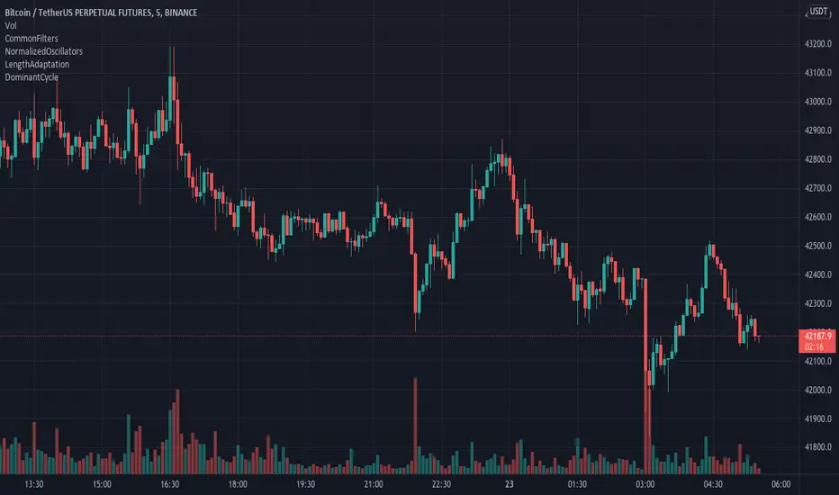
Madrid Bull Bear SentimentThis is an upgrade from Pinescript 1.0 published on April 2016 to Pinescript 5.0

Bitcoin Bull Runs Mid Cycle Aligned This script plots 2 lines which are the 2013 and 2016 bull run. The plots are aligned on their mid cycles to the 2021 mid cycle.
Settings:
You can move the plots on the x and y axis in the settings for the Daily, Weekly and Monthly TFs.
The plot is weird on the Monthly TF, best to use the Daily and Weekly.
If it doesn't load at first you have to zoom out fully and go back to 2013 for it to load. Then it will load.
[laoowai]BNB_USDT_3m_3Commas_Bollinger_MACD_RSI_StrategyBNB_USDT _3m
Release Notes:
Time: 3min
Pair: BNB_USDT
Use: {{strategy.order.alert_message}}
What's the difference with 3Commas Bollinger Strategy by tedwardd:
1. Initial capital: 1210 USDT (10$ Base order / 400$*3 Safety order), if you will change, please change JUST safety order volume or number of safety orders 2-3
2. Using just 2(3) safety order (original script 4)
3. More high-performance strategy for BNB_USDT
4. Using MACD to sell order (original script take profit by scale), thanks Drun30 .
5. Using RSI to analyze the market conditions.
Need to change:
bot_id = input(title="3Commas Bot ID", defval=" YOUR DATA ")
email_token = input(title="Bot Email Token", defval=" YOUR DATA ")
---------------------------------------------------------------------------------------------------------------------------------------------------------------------------------------------------
FAQ copy from tedwardd
---------------------------------------------------------------------------------------------------------------------------------------------------------------------------------------------------
This strategy is intended for use as a way of backtesting various parameters available on 3commas.
The primary inputs for the strategy are:
---------------------------------------------------------------------------------------------------------------------------------------------------------------------------------------------------
// USER INPUTS
Short MA Window - The length of the Short moving average
Long MA Window - The length of the Long moving average
Upper Band Offset - The offset to use for the upper bollinger offset
Lower Band Offset - The offset to use for the lower bollinger offset
Long Stop Loss % - The stop loss percentage to test
Long Take Profit % - The Take profit percentage to test
Initial SO Deviation % - The price deviation percentage required to place to first safety order
Safety Order Vol Step % - The volume scale to test
3Commas Bot ID - (self-explanatory)
Bot Email Token - Found in the deal start message for your bot (see link in the previous section for details)
3Commas Bot Trading Pair - The pair to include for composite bot start deals (should match the format of 3commas, not TradingView IE. USDT_BTC not BTCUSDT )
---------------------------------------------------------------------------------------------------------------------------------------------------------------------------------------------------
Start Date, Month, Year and End Date, Month, and Year all apply to the backtesting window. By default, it will use as much data as it can give the current period select (there is less historical data available for periods below 1H) back as far as 2016 (there appears to be no historical data on Trading view much before this). If you would like to test a different period of time, just change these values accordingly.
---------------------------------------------------------------------------------------------------------------------------------------------------------------------------------------------------
Composite bot using a Bollinger band type trading strategy. While its primary intention is to provide users a way of backtesting bot parameters, it can also be used to trigger a deal start by either using the {{strategy.order.alert_message}} field in your alert and providing the bot details in the configuration screen for the strategy or by including the usual deal start message provided by 3commas.
---------------------------------------------------------------------------------------------------------------------------------------------------------------------------------------------------
Original script:
1. 3Commas Bollinger Strategy by tedwardd
2. Momentum Strategy ( BTC /USDT; 1h) - MACD (with source code) by Drun30

3Commas Bollinger StrategyThis strategy is intended for use as a way of backtesting various parameters available on 3commas.io composite bot using a bollinger band type trading strategy. While it's primary intention is to provide users a way of backtesting bot parameters, it can also be used to trigger a deal start by either using the {{strategy.open.alert_message}} field in your alert and providing the bot details in the configuration screen for the strategy or by including the usual deal start message provided by 3commas. You can find more information about how to do this from help.3commas.io
The primary inputs for the strategy are:
// USER INPUTS
Short MA Window - The length of the Short moving average
Long MA Window - The length of the Long moving average
Upper Band Offset - The offset to use for the upper bollinger offset
Lower Band Offset - The offset to use for the lower bollinger offset
Long Stop Loss % - The stop loss percentage to test
Long Take Profit % - The Take profit percentage to test
Initial SO Deviation % - The price deviation percentage required to place to first safety order
Safety Order Vol Step % - The volume scale to test
3Commas Bot ID - (self explanatory)
Bot Email Token - Found in the deal start message for your bot (see link in previous section for details)
3Commas Bot Trading Pair - The pair to include for composite bot start deals (should match format of 3commas, not TradingView IE. USDT_BTC not BTCUSDT)
Start Date, Month, Year and End Date, Month and Year all apply to the backtesting window. By default it will use as much data as it can given the current period select (there is less historical data available for periods below 1H) back as far as 2016 (there appears to be no historical data on Trading view much before this). If you would like to test a different period of time, just change these values accordingly.
Known Issues
Currently there are a couple of issues with this strategy that you should be aware of. I may fix them at some point in the future but they don't really bug me so this is more for informational purposes than a promise that they may one day be fixed.
Does not test trailing take profit
Number of safety orders and Safety Order Step Scale are currently not user configurable (must edit source code)
Using the user configuration to generate deal start message assumes you are triggering a composite bot, not a simple bot.

CV_VWAP_GMECoefficient of variance GME ‰
Gray area: Regional price variance of GME in per milles
Light gray thick line: NYSE:GME deviation from global mean
1. Select a chart 24-hour ticker like FX_IDC:USDEUR
2. Select a timescale (5 min, 15 min, ...)
3. Monitor the regional price variance
Exchanges included: NYSE, XETR, BMV, FWB, SWB, BITTREX, FTX
Currency conversion: Forex
Adapted from Detecting the great short squeeze on Volkswagen, Godfrey, K. (2016, February 18).