MTF RSI CandlesThis Pine Script indicator is designed to provide a visual representation of Relative Strength Index (RSI) values across multiple timeframes. It enhances traditional candlestick charts by color-coding candles based on RSI levels, offering a clearer picture of overbought, oversold, and sideways market conditions. Additionally, it displays a hoverable table with RSI values for multiple predefined timeframes.
Key Features
1. Candle Coloring Based on RSI Levels:
Candles are color-coded based on predefined RSI ranges for easy interpretation of market conditions.
RSI Levels:
75-100: Strongest Overbought (Green)
65-75: Stronger Overbought (Dark Green)
55-65: Overbought (Teal)
45-55: Sideways (Gray)
35-45: Oversold (Light Red)
25-35: Stronger Oversold (Dark Red)
0-25: Strongest Oversold (Bright Red)
2. Multi-Timeframe RSI Table:
Displays RSI values for the following timeframes:
1 Min, 2 Min, 3 Min, 4 Min, 5 Min
10 Min, 15 Min, 30 Min, 1 Hour, 1 Day, 1 Week
Helps traders identify RSI trends across different time horizons.
3. Hoverable RSI Values:
Displays the RSI value of any candle when hovering over it, providing additional insights for analysis.
Inputs
1. RSI Length:
Default: 14
Determines the calculation period for the RSI indicator.
2. RSI Levels:
Configurable thresholds for RSI zones:
75-100: Strongest Overbought
65-75: Stronger Overbought
55-65: Overbought
45-55: Sideways
35-45: Oversold
25-35: Stronger Oversold
0-25: Strongest Oversold
How It Works:
1. RSI Calculation:
The RSI is calculated for the current timeframe using the input RSI Length.
It is also computed for 11 additional predefined timeframes using request.security.
2. Candle Coloring:
Candles are colored based on their RSI values and the specified RSI levels.
3. Hoverable RSI Values:
Each candle displays its RSI value when hovered over, via a dynamically created label.
Multi-Timeframe Table:
A table at the bottom-left of the chart displays RSI values for all predefined timeframes, making it easy to compare trends.
Usage:
1. Trend Identification:
Use candle colors to quickly assess market conditions (overbought, oversold, or sideways).
2. Timeframe Analysis:
Compare RSI values across different timeframes to determine long-term and short-term momentum.
3. Signal Confirmation:
Combine RSI signals with other indicators or patterns for higher-confidence trades.
Best Practices
Use this indicator in conjunction with volume analysis, support/resistance levels, or trendline strategies for better results.
Customize RSI levels and timeframes based on your trading strategy or market conditions.
Limitations
RSI is a lagging indicator and may not always predict immediate market reversals.
Multi-timeframe analysis can lead to conflicting signals; consider your trading horizon.
Cari skrip untuk "汇丰股票25"

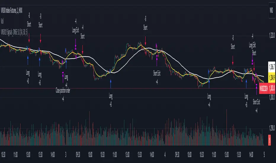
DNSE VN301!, SMA & EMA Cross StrategyDiscover the tailored Pinescript to trade VN30F1M Future Contracts intraday, the strategy focuses on SMA & EMA crosses to identify potential entry/exit points. The script closes all positions by 14:25 to avoid holding any contracts overnight.
HNX:VN301!
www.tradingview.com
Setting & Backtest result:
1-minute chart, initial capital of VND 100 million, entering 4 contracts per time, backtest result from Jan-2024 to Nov-2024 yielded a return over 40%, executed over 1,000 trades (average of 4 trades/day), winning trades rate ~ 30% with a profit factor of 1.10.
The default setting of the script:
A decent optimization is reached when SMA and EMA periods are set to 60 and 15 respectively while the Long/Short stop-loss level is set to 20 ticks (2 points) from the entry price.
Entry & Exit conditions:
Long signals are generated when ema(15) crosses over sma(60) while Short signals happen when ema(15) crosses under sma(60). Long orders are closed when ema(15) crosses under sma(60) while Short orders are closed when ema(15) crosses over sma(60).
Exit conditions happen when (whichever came first):
Another Long/Short signal is generated
The Stop-loss level is reached
The Cut-off time is reached (14:25 every day)
*Disclaimers:
Futures Contracts Trading are subjected to a high degree of risk and price movements can fluctuate significantly. This script functions as a reference source and should be used after users have clearly understood how futures trading works, accessed their risk tolerance level, and are knowledgeable of the functioning logic behind the script.
Users are solely responsible for their investment decisions, and DNSE is not responsible for any potential losses from applying such a strategy to real-life trading activities. Past performance is not indicative/guarantee of future results, kindly reach out to us should you have specific questions about this script.
---------------------------------------------------------------------------------------
Khám phá Pinescript được thiết kế riêng để giao dịch Hợp đồng tương lai VN30F1M trong ngày, chiến lược tập trung vào các đường SMA & EMA cắt nhau để xác định các điểm vào/ra tiềm năng. Chiến lược sẽ đóng tất cả các vị thế trước 14:25 để tránh giữ bất kỳ hợp đồng nào qua đêm.
Thiết lập & Kết quả backtest:
Chart 1 phút, vốn ban đầu là 100 triệu đồng, vào 4 hợp đồng mỗi lần, kết quả backtest từ tháng 1/2024 tới tháng 11/2024 mang lại lợi nhuận trên 40%, thực hiện hơn 1.000 giao dịch (trung bình 4 giao dịch/ngày), tỷ lệ giao dịch thắng ~ 30% với hệ số lợi nhuận là 1,10.
Thiết lập mặc định của chiến lược:
Đạt được một mức tối ưu ổn khi SMA và EMA periods được đặt lần lượt là 60 và 15 trong khi mức cắt lỗ được đặt thành 20 tick (2 điểm) từ giá vào.
Điều kiện Mở và Đóng vị thế:
Tín hiệu Long được tạo ra khi ema(15) cắt trên sma(60) trong khi tín hiệu Short xảy ra khi ema(15) cắt dưới sma(60). Lệnh Long được đóng khi ema(15) cắt dưới sma(60) trong khi lệnh Short được đóng khi ema(15) cắt lên sma(60).
Điều kiện đóng vị thể xảy ra khi (tùy điều kiện nào đến trước):
Một tín hiệu Long/Short khác được tạo ra
Giá chạm mức cắt lỗ
Lệnh chưa đóng nhưng tới giờ cut-off (14:25 hàng ngày)
*Tuyên bố miễn trừ trách nhiệm:
Giao dịch hợp đồng tương lai có mức rủi ro cao và giá có thể dao động đáng kể. Chiến lược này hoạt động như một nguồn tham khảo và nên được sử dụng sau khi người dùng đã hiểu rõ cách thức giao dịch hợp đồng tương lai, đã đánh giá mức độ chấp nhận rủi ro của bản thân và hiểu rõ về logic vận hành của chiến lược này.
Người dùng hoàn toàn chịu trách nhiệm về các quyết định đầu tư của mình và DNSE không chịu trách nhiệm về bất kỳ khoản lỗ tiềm ẩn nào khi áp dụng chiến lược này vào các hoạt động giao dịch thực tế. Hiệu suất trong quá khứ không chỉ ra/cam kết kết quả trong tương lai, vui lòng liên hệ với chúng tôi nếu bạn có thắc mắc cụ thể về chiến lược giao dịch này.
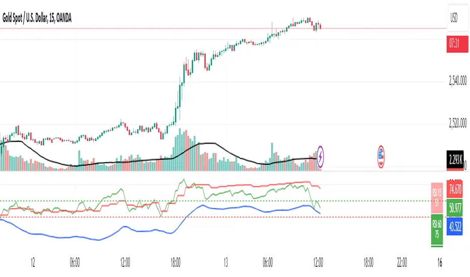
RSI 15/60 and ADX PlotIn this script, the buy and sell criteria are based on the Relative Strength Index (RSI) values calculated for two different timeframes: the 15-minute RSI and the hourly RSI. These timeframes are used together to check signals when certain thresholds are crossed, providing confirmation across both short-term and longer-term momentum.
Buy Criteria:
Condition 1:
Hourly RSI > 60: This means the longer-term momentum shows strength.
15-minute RSI crosses above 60: This shows that the shorter-term momentum is catching up and confirms increasing strength.
Condition 2:
15-minute RSI > 60: This indicates that the short-term trend is already strong.
Hourly RSI crosses above 60: This confirms that the longer-term trend is also gaining strength.
Both conditions aim to capture the moments when the market shows increasing strength across both short and long timeframes, signaling a potential buy opportunity.
Sell Criteria:
Condition 1:
Hourly RSI < 40: This indicates that the longer-term trend is weakening.
15-minute RSI crosses below 40: The short-term momentum is also turning down, confirming the weakening trend.
Condition 2:
15-minute RSI < 40: The short-term trend is already weak.
Hourly RSI crosses below 40: The longer-term trend is now confirming the weakness, indicating a potential sell.
These conditions work to identify when the market is showing weakness in both short-term and long-term timeframes, signaling a potential sell opportunity.
ADX Confirmation :
The Average Directional Index (ADX) is a key tool for measuring the strength of a trend. It can be used alongside the RSI to confirm whether a buy or sell signal is occurring in a strong trend or during market consolidation. Here's how ADX can be integrated:
ADX > 25: This indicates a strong trend. Using this threshold, you can confirm buy or sell signals when there is a strong upward or downward movement in the market.
Buy Example: If a buy signal (RSI > 60) is triggered and the ADX is above 25, this confirms that the market is in a strong uptrend, making the buy signal more reliable.
Sell Example: If a sell signal (RSI < 40) is triggered and the ADX is above 25, it confirms a strong downtrend, validating the sell signal.
ADX < 25: This suggests a weak or non-existent trend. In this case, RSI signals might be less reliable since the market could be moving sideways.
Final Approach:
The RSI criteria help identify potential overbought and oversold conditions in both short and long timeframes.
The ADX confirmation ensures that the signals generated are happening during strong trends, increasing the likelihood of successful trades by filtering out weak or choppy market conditions.
This combination of RSI and ADX can help traders make more informed decisions by ensuring both momentum and trend strength align before entering or exiting trades.
Average Directional Index with MACombining the Average Directional Index (ADX) with a 14-period Exponential Moving Average (EMA) can provide traders with a comprehensive approach to identify both the strength of a trend (through ADX) and the trend's direction (using EMA). Let's break down each component and then discuss how they can be combined:
Average Directional Index (ADX):
The ADX is a technical indicator that measures the strength or momentum of a trend, regardless of its direction. The ADX is derived from two other indicators:
Positive Directional Index (+DI): Measures the strength of upward price movement.
Negative Directional Index (-DI): Measures the strength of downward price movement.
14-period Exponential Moving Average (EMA):
The 14-period EMA is a trend-following indicator that gives more weight to recent price data compared to simple moving averages (SMAs). The EMA is calculated by taking the average of the last 14 closing prices, giving more importance to the most recent prices.
Combining ADX and EMA:
When combining ADX with a 14-period EMA:
ADX as a Filter:
Traders might use the ADX to filter out trades when the trend's strength is weak (e.g., ADX below 25) to avoid trading in sideways or choppy markets.
EMA for Trend Direction:
Traders can use the 14-period EMA to determine the trend direction.
A price above the 14-period EMA might indicate an uptrend, while a price below the EMA might suggest a downtrend.
Example Strategy:
Here's a simplified trading strategy combining ADX and EMA:
Trend Identification:
Buy when the price is above the 14-period EMA and the ADX indicates a strong uptrend (e.g., ADX > 25).
Sell or go short when the price is below the 14-period EMA and the ADX indicates a strong downtrend (e.g., ADX > 25).
Avoid Choppy Markets:
Avoid trading when the ADX is below a certain threshold (e.g., ADX < 25) to filter out sideways or range-bound markets.
Combining ADX and a 14-period EMA can provide traders with a balanced approach to identify both the strength and direction of a trend. However, it's essential to remember that no indicator or strategy can guarantee profits, and it's crucial to use risk management techniques and other tools to make informed trading decisions. Consider back testing this strategy on historical data and adjusting the parameters based on their trading style and risk tolerance.

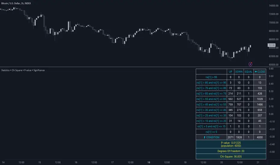
Statistics • Chi Square • P-value • SignificanceThe Statistics • Chi Square • P-value • Significance publication aims to provide a tool for combining different conditions and checking whether the outcome is significant using the Chi-Square Test and P-value.
🔶 USAGE
The basic principle is to compare two or more groups and check the results of a query test, such as asking men and women whether they want to see a romantic or non-romantic movie.
–––––––––––––––––––––––––––––––––––––––––––––
| | ROMANTIC | NON-ROMANTIC | ⬅︎ MOVIE |
–––––––––––––––––––––––––––––––––––––––––––––
| MEN | 2 | 8 | 10 |
–––––––––––––––––––––––––––––––––––––––––––––
| WOMEN | 7 | 3 | 10 |
–––––––––––––––––––––––––––––––––––––––––––––
|⬆︎ SEX | 10 | 10 | 20 |
–––––––––––––––––––––––––––––––––––––––––––––
We calculate the Chi-Square Formula, which is:
Χ² = Σ ( (Observed Value − Expected Value)² / Expected Value )
In this publication, this is:
chiSquare = 0.
for i = 0 to rows -1
for j = 0 to colums -1
observedValue = aBin.get(i).aFloat.get(j)
expectedValue = math.max(1e-12, aBin.get(i).aFloat.get(colums) * aBin.get(rows).aFloat.get(j) / sumT) //Division by 0 protection
chiSquare += math.pow(observedValue - expectedValue, 2) / expectedValue
Together with the 'Degree of Freedom', which is (rows − 1) × (columns − 1) , the P-value can be calculated.
In this case it is P-value: 0.02462
A P-value lower than 0.05 is considered to be significant. Statistically, women tend to choose a romantic movie more, while men prefer a non-romantic one.
Users have the option to choose a P-value, calculated from a standard table or through a math.ucla.edu - Javascript-based function (see references below).
Note that the population (10 men + 10 women = 20) is small, something to consider.
Either way, this principle is applied in the script, where conditions can be chosen like rsi, close, high, ...
🔹 CONDITION
Conditions are added to the left column ('CONDITION')
For example, previous rsi values (rsi ) between 0-100, divided in separate groups
🔹 CLOSE
Then, the movement of the last close is evaluated
UP when close is higher then previous close (close )
DOWN when close is lower then previous close
EQUAL when close is equal then previous close
It is also possible to use only 2 columns by adding EQUAL to UP or DOWN
UP
DOWN/EQUAL
or
UP/EQUAL
DOWN
In other words, when previous rsi value was between 80 and 90, this resulted in:
19 times a current close higher than previous close
14 times a current close lower than previous close
0 times a current close equal than previous close
However, the P-value tells us it is not statistical significant.
NOTE: Always keep in mind that past behaviour gives no certainty about future behaviour.
A vertical line is drawn at the beginning of the chosen population (max 4990)
Here, the results seem significant.
🔹 GROUPS
It is important to ensure that the groups are formed correctly. All possibilities should be present, and conditions should only be part of 1 group.
In the example above, the two top situations are acceptable; close against close can only be higher, lower or equal.
The two examples at the bottom, however, are very poorly constructed.
Several conditions can be placed in more than 1 group, and some conditions are not integrated into a group. Even if the results are significant, they are useless because of the group formation.
A population count is added as an aid to spot errors in group formation.
In this example, there is a discrepancy between the population and total count due to the absence of a condition.
The results when rsi was between 5-25 are not included, resulting in unreliable results.
🔹 PRACTICAL EXAMPLES
In this example, we have specific groups where the condition only applies to that group.
For example, the condition rsi > 55 and rsi <= 65 isn't true in another group.
Also, every possible rsi value (0 - 100) is present in 1 of the groups.
rsi > 15 and rsi <= 25 28 times UP, 19 times DOWN and 2 times EQUAL. P-value: 0.01171
When looking in detail and examining the area 15-25 RSI, we see this:
The population is now not representative (only checking for RSI between 15-25; all other RSI values are not included), so we can ignore the P-value in this case. It is merely to check in detail. In this case, the RSI values 23 and 24 seem promising.
NOTE: We should check what the close price did without any condition.
If, for example, the close price had risen 100 times out of 100, this would make things very relative.
In this case (at least two conditions need to be present), we set 1 condition at 'always true' and another at 'always false' so we'll get only the close values without any condition:
Changing the population or the conditions will change the P-value.
In the following example, the outcome is evaluated when:
close value from 1 bar back is higher than the close value from 2 bars back
close value from 1 bar back is lower/equal than the close value from 2 bars back
Or:
close value from 1 bar back is higher than the close value from 2 bars back
close value from 1 bar back is equal than the close value from 2 bars back
close value from 1 bar back is lower than the close value from 2 bars back
In both examples, all possibilities of close against close are included in the calculations. close can only by higher, equal or lower than close
Both examples have the results without a condition included (5 = 5 and 5 < 5) so one can compare the direction of current close.
🔶 NOTES
• Always keep in mind that:
Past behaviour gives no certainty about future behaviour.
Everything depends on time, cycles, events, fundamentals, technicals, ...
• This test only works for categorical data (data in categories), such as Gender {Men, Women} or color {Red, Yellow, Green, Blue} etc., but not numerical data such as height or weight. One might argue that such tests shouldn't use rsi, close, ... values.
• Consider what you're measuring
For example rsi of the current bar will always lead to a close higher than the previous close, since this is inherent to the rsi calculations.
• Be careful; often, there are na -values at the beginning of the series, which are not included in the calculations!
• Always keep in mind considering what the close price did without any condition
• The numbers must be large enough. Each entry must be five or more. In other words, it is vital to make the 'population' large enough.
• The code can be developed further, for example, by splitting UP, DOWN in close UP 1-2%, close UP 2-3%, close UP 3-4%, ...
• rsi can be supplemented with stochRSI, MFI, sma, ema, ...
🔶 SETTINGS
🔹 Population
• Choose the population size; in other words, how many bars you want to go back to. If fewer bars are available than set, this will be automatically adjusted.
🔹 Inputs
At least two conditions need to be chosen.
• Users can add up to 11 conditions, where each condition can contain two different conditions.
🔹 RSI
• Length
🔹 Levels
• Set the used levels as desired.
🔹 Levels
• P-value: P-value retrieved using a standard table method or a function.
• Used function, derived from Chi-Square Distribution Function; JavaScript
LogGamma(Z) =>
S = 1
+ 76.18009173 / Z
- 86.50532033 / (Z+1)
+ 24.01409822 / (Z+2)
- 1.231739516 / (Z+3)
+ 0.00120858003 / (Z+4)
- 0.00000536382 / (Z+5)
(Z-.5) * math.log(Z+4.5) - (Z+4.5) + math.log(S * 2.50662827465)
Gcf(float X, A) => // Good for X > A +1
A0=0., B0=1., A1=1., B1=X, AOLD=0., N=0
while (math.abs((A1-AOLD)/A1) > .00001)
AOLD := A1
N += 1
A0 := A1+(N-A)*A0
B0 := B1+(N-A)*B0
A1 := X*A0+N*A1
B1 := X*B0+N*B1
A0 := A0/B1
B0 := B0/B1
A1 := A1/B1
B1 := 1
Prob = math.exp(A * math.log(X) - X - LogGamma(A)) * A1
1 - Prob
Gser(X, A) => // Good for X < A +1
T9 = 1. / A
G = T9
I = 1
while (T9 > G* 0.00001)
T9 := T9 * X / (A + I)
G := G + T9
I += 1
G *= math.exp(A * math.log(X) - X - LogGamma(A))
Gammacdf(x, a) =>
GI = 0.
if (x<=0)
GI := 0
else if (x
Chisqcdf = Gammacdf(Z/2, DF/2)
Chisqcdf := math.round(Chisqcdf * 100000) / 100000
pValue = 1 - Chisqcdf
🔶 REFERENCES
mathsisfun.com, Chi-Square Test
Chi-Square Distribution Function
Incomplete Session Candle - Incomplete Timeframe Candle Marker The "Incomplete Session Candle - Incomplete Timeframe Candle Marker" is an advanced tool tailored for technical analysts who understand the importance of accurate timeframes in their charting. While the indicator is not limited to the Indian market, its genesis is rooted in the nuances of trading sessions like those in India, which span 375 minutes from 9:15 AM to 3:30 PM.
Key Features:
Detects if the current timeframe is intraday (minutes or hours).
Calculates the expected duration of the candle for the chosen timeframe.
Highlights candles that don't achieve their expected session duration by placing a cross shape above the bar.
Compatible across various intraday timeframes, aiding traders in spotting discrepancies promptly.
Why We Made This: Not Just for India:
While we looked at the Indian market, this indicator works everywhere. Regular timeframes like 30 minutes, 1 hour, and 2 hours often end with incomplete candles, especially at the end of the trading day. For example:
A 30-minute timeframe makes 13 candles, but the last one is only 15 minutes long.
A 1-hour timeframe shows 7 candles, but the last one is just the last 15 minutes.
By switching to different timeframes like 25 minutes, 75 minutes, and 125 minutes, you get more complete information for better trading decisions. Learn more about this in our article: "Power of 25, 75, and 125-Minute Timeframes in the Indian Market", recognized by Trading View's Editors' Pick.
Benefits:
The indicator extends its benefits even to users without access to certain timeframes. It accommodates traders using a 1-hour timeframe (pertaining to Indian traders). By employing this indicator, traders consistently remain mindful of incomplete candles within their chosen timeframe
For those who utilize concepts like RBR, RBD, DBR, and DBD, this indicator is paramount. An incomplete candle can skew analysis, leading to potential misinterpretations of base or leg candles.
Final thoughts:
In markets like the Indian stock market, adopting such a tool is not just beneficial, but necessary. Whether you have access to unconventional timeframes or are using traditional ones, recognizing and accounting for the limitations of incomplete candles is critical & it's important to know if your candles fit the timeframe properly. This indicator gives you a better view of the market, which helps you make smarter trades.
Lastly, Thank you for your support! Your likes & comments. If you want to give any feedback then you can give in comment section.
Let's conquer the markets together!

Any Oscillator Underlay [TTF]We are proud to release a new indicator that has been a while in the making - the Any Oscillator Underlay (AOU) !
Note: There is a lot to discuss regarding this indicator, including its intent and some of how it operates, so please be sure to read this entire description before using this indicator to help ensure you understand both the intent and some limitations with this tool.
Our intent for building this indicator was to accomplish the following:
Combine all of the oscillators that we like to use into a single indicator
Take up a bit less screen space for the underlay indicators for strategies that utilize multiple oscillators
Provide a tool for newer traders to be able to leverage multiple oscillators in a single indicator
Features:
Includes 8 separate, fully-functional indicators combined into one
Ability to easily enable/disable and configure each included indicator independently
Clearly named plots to support user customization of color and styling, as well as manual creation of alerts
Ability to customize sub-indicator title position and color
Ability to customize sub-indicator divider lines style and color
Indicators that are included in this initial release:
TSI
2x RSIs (dubbed the Twin RSI )
Stochastic RSI
Stochastic
Ultimate Oscillator
Awesome Oscillator
MACD
Outback RSI (Color-coding only)
Quick note on OB/OS:
Before we get into covering each included indicator, we first need to cover a core concept for how we're defining OB and OS levels. To help illustrate this, we will use the TSI as an example.
The TSI by default has a mid-point of 0 and a range of -100 to 100. As a result, a common practice is to place lines on the -30 and +30 levels to represent OS and OB zones, respectively. Most people tend to view these levels as distance from the edges/outer bounds or as absolute levels, but we feel a more way to frame the OB/OS concept is to instead define it as distance ("offset") from the mid-line. In keeping with the -30 and +30 levels in our example, the offset in this case would be "30".
Taking this a step further, let's say we decided we wanted an offset of 25. Since the mid-point is 0, we'd then calculate the OB level as 0 + 25 (+25), and the OS level as 0 - 25 (-25).
Now that we've covered the concept of how we approach defining OB and OS levels (based on offset/distance from the mid-line), and since we did apply some transformations, rescaling, and/or repositioning to all of the indicators noted above, we are going to discuss each component indicator to detail both how it was modified from the original to fit the stacked-indicator model, as well as the various major components that the indicator contains.
TSI:
This indicator contains the following major elements:
TSI and TSI Signal Line
Color-coded fill for the TSI/TSI Signal lines
Moving Average for the TSI
TSI Histogram
Mid-line and OB/OS lines
Default TSI fill color coding:
Green : TSI is above the signal line
Red : TSI is below the signal line
Note: The TSI traditionally has a range of -100 to +100 with a mid-point of 0 (range of 200). To fit into our stacking model, we first shrunk the range to 100 (-50 to +50 - cut it in half), then repositioned it to have a mid-point of 50. Since this is the "bottom" of our indicator-stack, no additional repositioning is necessary.
Twin RSI:
This indicator contains the following major elements:
Fast RSI (useful if you want to leverage 2x RSIs as it makes it easier to see the overlaps and crosses - can be disabled if desired)
Slow RSI (primary RSI)
Color-coded fill for the Fast/Slow RSI lines (if Fast RSI is enabled and configured)
Moving Average for the Slow RSI
Mid-line and OB/OS lines
Default Twin RSI fill color coding:
Dark Red : Fast RSI below Slow RSI and Slow RSI below Slow RSI MA
Light Red : Fast RSI below Slow RSI and Slow RSI above Slow RSI MA
Dark Green : Fast RSI above Slow RSI and Slow RSI below Slow RSI MA
Light Green : Fast RSI above Slow RSI and Slow RSI above Slow RSI MA
Note: The RSI naturally has a range of 0 to 100 with a mid-point of 50, so no rescaling or transformation is done on this indicator. The only manipulation done is to properly position it in the indicator-stack based on which other indicators are also enabled.
Stochastic and Stochastic RSI:
These indicators contain the following major elements:
Configurable lengths for the RSI (for the Stochastic RSI only), K, and D values
Configurable base price source
Mid-line and OB/OS lines
Note: The Stochastic and Stochastic RSI both have a normal range of 0 to 100 with a mid-point of 50, so no rescaling or transformations are done on either of these indicators. The only manipulation done is to properly position it in the indicator-stack based on which other indicators are also enabled.
Ultimate Oscillator (UO):
This indicator contains the following major elements:
Configurable lengths for the Fast, Middle, and Slow BP/TR components
Mid-line and OB/OS lines
Moving Average for the UO
Color-coded fill for the UO/UO MA lines (if UO MA is enabled and configured)
Default UO fill color coding:
Green : UO is above the moving average line
Red : UO is below the moving average line
Note: The UO naturally has a range of 0 to 100 with a mid-point of 50, so no rescaling or transformation is done on this indicator. The only manipulation done is to properly position it in the indicator-stack based on which other indicators are also enabled.
Awesome Oscillator (AO):
This indicator contains the following major elements:
Configurable lengths for the Fast and Slow moving averages used in the AO calculation
Configurable price source for the moving averages used in the AO calculation
Mid-line
Option to display the AO as a line or pseudo-histogram
Moving Average for the AO
Color-coded fill for the AO/AO MA lines (if AO MA is enabled and configured)
Default AO fill color coding (Note: Fill was disabled in the image above to improve clarity):
Green : AO is above the moving average line
Red : AO is below the moving average line
Note: The AO is technically has an infinite (unbound) range - -∞ to ∞ - and the effective range is bound to the underlying security price (e.g. BTC will have a wider range than SP500, and SP500 will have a wider range than EUR/USD). We employed some special techniques to rescale this indicator into our desired range of 100 (-50 to 50), and then repositioned it to have a midpoint of 50 (range of 0 to 100) to meet the constraints of our stacking model. We then do one final repositioning to place it in the correct position the indicator-stack based on which other indicators are also enabled. For more details on how we accomplished this, read our section "Binding Infinity" below.
MACD:
This indicator contains the following major elements:
Configurable lengths for the Fast and Slow moving averages used in the MACD calculation
Configurable price source for the moving averages used in the MACD calculation
Configurable length and calculation method for the MACD Signal Line calculation
Mid-line
Note: Like the AO, the MACD also technically has an infinite (unbound) range. We employed the same principles here as we did with the AO to rescale and reposition this indicator as well. For more details on how we accomplished this, read our section "Binding Infinity" below.
Outback RSI (ORSI):
This is a stripped-down version of the Outback RSI indicator (linked above) that only includes the color-coding background (suffice it to say that it was not technically feasible to attempt to rescale the other components in a way that could consistently be clearly seen on-chart). As this component is a bit of a niche/special-purpose sub-indicator, it is disabled by default, and we suggest it remain disabled unless you have some pre-defined strategy that leverages the color-coding element of the Outback RSI that you wish to use.
Binding Infinity - How We Incorporated the AO and MACD (Warning - Math Talk Ahead!)
Note: This applies only to the AO and MACD at time of original publication. If any other indicators are added in the future that also fall into the category of "binding an infinite-range oscillator", we will make that clear in the release notes when that new addition is published.
To help set the stage for this discussion, it's important to note that the broader challenge of "equalizing inputs" is nothing new. In fact, it's a key element in many of the most popular fields of data science, such as AI and Machine Learning. They need to take a diverse set of inputs with a wide variety of ranges and seemingly-random inputs (referred to as "features"), and build a mathematical or computational model in order to work. But, when the raw inputs can vary significantly from one another, there is an inherent need to do some pre-processing to those inputs so that one doesn't overwhelm another simply due to the difference in raw values between them. This is where feature scaling comes into play.
With this in mind, we implemented 2 of the most common methods of Feature Scaling - Min-Max Normalization (which we call "Normalization" in our settings), and Z-Score Normalization (which we call "Standardization" in our settings). Let's take a look at each of those methods as they have been implemented in this script.
Min-Max Normalization (Normalization)
This is one of the most common - and most basic - methods of feature scaling. The basic formula is: y = (x - min)/(max - min) - where x is the current data sample, min is the lowest value in the dataset, and max is the highest value in the dataset. In this transformation, the max would evaluate to 1, and the min would evaluate to 0, and any value in between the min and the max would evaluate somewhere between 0 and 1.
The key benefits of this method are:
It can be used to transform datasets of any range into a new dataset with a consistent and known range (0 to 1).
It has no dependency on the "shape" of the raw input dataset (i.e. does not assume the input dataset can be approximated to a normal distribution).
But there are a couple of "gotchas" with this technique...
First, it assumes the input dataset is complete, or an accurate representation of the population via random sampling. While in most situations this is a valid assumption, in trading indicators we don't really have that luxury as we're often limited in what sample data we can access (i.e. number of historical bars available).
Second, this method is highly sensitive to outliers. Since the crux of this transformation is based on the max-min to define the initial range, a single significant outlier can result in skewing the post-transformation dataset (i.e. major price movement as a reaction to a significant news event).
You can potentially mitigate those 2 "gotchas" by using a mechanism or technique to find and discard outliers (e.g. calculate the mean and standard deviation of the input dataset and discard any raw values more than 5 standard deviations from the mean), but if your most recent datapoint is an "outlier" as defined by that algorithm, processing it using the "scrubbed" dataset would result in that new datapoint being outside the intended range of 0 to 1 (e.g. if the new datapoint is greater than the "scrubbed" max, it's post-transformation value would be greater than 1). Even though this is a bit of an edge-case scenario, it is still sure to happen in live markets processing live data, so it's not an ideal solution in our opinion (which is why we chose not to attempt to discard outliers in this manner).
Z-Score Normalization (Standardization)
This method of rescaling is a bit more complex than the Min-Max Normalization method noted above, but it is also a widely used process. The basic formula is: y = (x – μ) / σ - where x is the current data sample, μ is the mean (average) of the input dataset, and σ is the standard deviation of the input dataset. While this transformation still results in a technically-infinite possible range, the output of this transformation has a 2 very significant properties - the mean (average) of the output dataset has a mean (μ) of 0 and a standard deviation (σ) of 1.
The key benefits of this method are:
As it's based on normalizing the mean and standard deviation of the input dataset instead of a linear range conversion, it is far less susceptible to outliers significantly affecting the result (and in fact has the effect of "squishing" outliers).
It can be used to accurately transform disparate sets of data into a similar range regardless of the original dataset's raw/actual range.
But there are a couple of "gotchas" with this technique as well...
First, it still technically does not do any form of range-binding, so it is still technically unbounded (range -∞ to ∞ with a mid-point of 0).
Second, it implicitly assumes that the raw input dataset to be transformed is normally distributed, which won't always be the case in financial markets.
The first "gotcha" is a bit of an annoyance, but isn't a huge issue as we can apply principles of normal distribution to conceptually limit the range by defining a fixed number of standard deviations from the mean. While this doesn't totally solve the "infinite range" problem (a strong enough sudden move can still break out of our "conceptual range" boundaries), the amount of movement needed to achieve that kind of impact will generally be pretty rare.
The bigger challenge is how to deal with the assumption of the input dataset being normally distributed. While most financial markets (and indicators) do tend towards a normal distribution, they are almost never going to match that distribution exactly. So let's dig a bit deeper into distributions are defined and how things like trending markets can affect them.
Skew (skewness): This is a measure of asymmetry of the bell curve, or put another way, how and in what way the bell curve is disfigured when comparing the 2 halves. The easiest way to visualize this is to draw an imaginary vertical line through the apex of the bell curve, then fold the curve in half along that line. If both halves are exactly the same, the skew is 0 (no skew/perfectly symmetrical) - which is what a normal distribution has (skew = 0). Most financial markets tend to have short, medium, and long-term trends, and these trends will cause the distribution curve to skew in one direction or another. Bullish markets tend to skew to the right (positive), and bearish markets to the left (negative).
Kurtosis: This is a measure of the "tail size" of the bell curve. Another way to state this could be how "flat" or "steep" the bell-shape is. If the bell is steep with a strong drop from the apex (like a steep cliff), it has low kurtosis. If the bell has a shallow, more sweeping drop from the apex (like a tall hill), is has high kurtosis. Translating this to financial markets, kurtosis is generally a metric of volatility as the bell shape is largely defined by the strength and frequency of outliers. This is effectively a measure of volatility - volatile markets tend to have a high level of kurtosis (>3), and stable/consolidating markets tend to have a low level of kurtosis (<3). A normal distribution (our reference), has a kurtosis value of 3.
So to try and bring all that back together, here's a quick recap of the Standardization rescaling method:
The Standardization method has an assumption of a normal distribution of input data by using the mean (average) and standard deviation to handle the transformation
Most financial markets do NOT have a normal distribution (as discussed above), and will have varying degrees of skew and kurtosis
Q: Why are we still favoring the Standardization method over the Normalization method, and how are we accounting for the innate skew and/or kurtosis inherent in most financial markets?
A: Well, since we're only trying to rescale oscillators that by-definition have a midpoint of 0, kurtosis isn't a major concern beyond the affect it has on the post-transformation scaling (specifically, the number of standard deviations from the mean we need to include in our "artificially-bound" range definition).
Q: So that answers the question about kurtosis, but what about skew?
A: So - for skew, the answer is in the formula - specifically the mean (average) element. The standard mean calculation assumes a complete dataset and therefore uses a standard (i.e. simple) average, but we're limited by the data history available to us. So we adapted the transformation formula to leverage a moving average that included a weighting element to it so that it favored recent datapoints more heavily than older ones. By making the average component more adaptive, we gained the effect of reducing the skew element by having the average itself be more responsive to recent movements, which significantly reduces the effect historical outliers have on the dataset as a whole. While this is certainly not a perfect solution, we've found that it serves the purpose of rescaling the MACD and AO to a far more well-defined range while still preserving the oscillator behavior and mid-line exceptionally well.
The most difficult parts to compensate for are periods where markets have low volatility for an extended period of time - to the point where the oscillators are hovering around the 0/midline (in the case of the AO), or when the oscillator and signal lines converge and remain close to each other (in the case of the MACD). It's during these periods where even our best attempt at ensuring accurate mirrored-behavior when compared to the original can still occasionally lead or lag by a candle.
Note: If this is a make-or-break situation for you or your strategy, then we recommend you do not use any of the included indicators that leverage this kind of bounding technique (the AO and MACD at time of publication) and instead use the Trandingview built-in versions!
We know this is a lot to read and digest, so please take your time and feel free to ask questions - we will do our best to answer! And as always, constructive feedback is always welcome!

SUPERTREND MIXED ICHI-DMI-DONCHIAN-VOL-GAP-HLBox@RLSUPERTREND MIXED ICHI-DMI-VOL-GAP-HLBox@RL
by RegisL76
This script is based on several trend indicators.
* ICHIMOKU (KINKO HYO)
* DMI (Directional Movement Index)
* SUPERTREND ICHIMOKU + SUPERTREND DMI
* DONCHIAN CANAL Optimized with Colored Bars
* HMA Hull
* Fair Value GAP
* VOLUME/ MA Volume
* PRICE / MA Price
* HHLL BOXES
All these indications are visible simultaneously on a single graph. A data table summarizes all the important information to make a good trade decision.
ICHIMOKU Indicator:
The ICHIMOKU indicator is visualized in the traditional way.
ICHIMOKU standard setting values are respected but modifiable. (Traditional defaults = .
An oriented visual symbol, near the last value, indicates the progression (Ascending, Descending or neutral) of the TENKAN-SEN and the KIJUN-SEN as well as the period used.
The CLOUD (KUMO) and the CHIKOU-SPAN are present and are essential for the complete analysis of the ICHIMOKU.
At the top of the graph are visually represented the crossings of the TENKAN and the KIJUN.
Vertical lines, accompanied by labels, make it possible to quickly visualize the particularities of the ICHIMOKU.
A line displays the current bar.
A line visualizes the end of the CLOUD (KUMO) which is shifted 25 bars into the future.
A line visualizes the end of the chikou-span, which is shifted 25 bars in the past.
DIRECTIONAL MOVEMENT INDEX (DMI) : Treated conventionally : DI+, DI-, ADX and associated with a SUPERTREND DMI.
A visual symbol at the bottom of the graph indicates DI+ and DI- crossings
A line of oriented and colored symbols (DMI Line) at the top of the chart indicates the direction and strength of the trend.
SUPERTREND ICHIMOKU + SUPERTREND DMI :
Trend following by SUPERTREND calculation.
DONCHIAN CHANNEL: Treated conventionally. (And optimized by colored bars when overshooting either up or down.
The lines, high and low of the last values of the channel are represented to quickly visualize the level of the RANGE.
SUPERTREND HMA (HULL) Treated conventionally.
The HMA line visually indicates, according to color and direction, the market trend.
A visual symbol at the bottom of the chart indicates opportunities to sell and buy.
VOLUME:
Calculation of the MOBILE AVERAGE of the volume with comparison of the volume compared to the moving average of the volume.
The indications are colored and commented according to the comparison.
PRICE: Calculation of the MOBILE AVERAGE of the price with comparison of the price compared to the moving average of the price.
The indications are colored and commented according to the comparison.
HHLL BOXES:
Visualizes in the form of a box, for a given period, the max high and min low values of the price.
The configuration allows taking into account the high and low wicks of the price or the opening and closing values.
FAIR VALUE GAP :
This indicator displays 'GAP' levels over the current time period and an optional higher time period.
The script takes into account the high/low values of the current bar and compares with the 2 previous bars.
The "gap" is generated from the lack of overlap between these bars. Bearish or bullish gaps are determined by whether the gap is above or below HmaPrice, as they tend to fill, and can be used as targets.
NOTE: FAIR VALUE GAP has no values displayed in the table and/or label.
Important information (DATA) relating to each indicator is displayed in real time in a table and/or a label.
Each information is commented and colored according to direction, value, comparison etc.
Each piece of information indicates the values of the current bar and the previous value (in "FULL" mode).
The other possible modes for viewing the table and/or the label allow a more synthetic view of the information ("CONDENSED" and "MINIMAL" modes).
In order not to overload the vision of the chart too much, the visualization box of the RANGE DONCHIAN, the vertical lines of the shifted marks of the ICHIMOKU, as well as the boxes of the HHLL Boxes indicator are only visualized intermittently (managed by an adjustable time delay ).
The "HISTORICAL INFO READING" configuration parameter set to zero (by default) makes it possible to read all the information of the current bar in progress (Bar #0). All other values allow to read the information of a historical bar. The value 1 reads the information of the bar preceding the current bar (-1). The value 10 makes it possible to read the information of the tenth bar behind (-10) compared to the current bar, etc.
At the bottom of the DATAS table and label, lights, red, green or white indicate quickly summarize the trend from the various indicators.
Each light represents the number of indicators with the same trend at a given time.
Green for a bullish trend, red for a bearish trend and white for a neutral trend.
The conditions for determining a trend are for each indicator:
SUPERTREND ICHIMOHU + DMI: the 2 Super trends together are either bullish or bearish.
Otherwise the signal is neutral.
DMI: 2 main conditions:
BULLISH if DI+ >= DI- and ADX >25.
BEARISH if DI+ < DI- and ADX >25.
NEUTRAL if the 2 conditions are not met.
ICHIMOKU: 3 main conditions:
BULLISH if PRICE above the cloud and TENKAN > KIJUN and GREEN CLOUD AHEAD.
BEARISH if PRICE below the cloud and TENKAN < KIJUN and RED CLOUD AHEAD.
The other additional conditions (Data) complete the analysis and are present for informational purposes of the trend and depend on the context.
DONCHIAN CHANNEL: 1 main condition:
BULLISH: the price has crossed above the HIGH DC line.
BEARISH: the price has gone below the LOW DC line.
NEUTRAL if the price is between the HIGH DC and LOW DC lines
The 2 other complementary conditions (Datas) complete the analysis:
HIGH DC and LOW DC are increasing, falling or stable.
SUPERTREND HMA HULL: The script determines several trend levels:
STRONG BUY, BUY, STRONG SELL, SELL AND NEUTRAL.
VOLUME: 3 trend levels:
VOLUME > MOVING AVERAGE,
VOLUME < MOVING AVERAGE,
VOLUME = MOVING AVERAGE.
PRICE: 3 trend levels:
PRICE > MOVING AVERAGE,
PRICE < MOVING AVERAGE,
PRICE = MOVING AVERAGE.
If you are using this indicator/strategy and you are satisfied with the results, you can possibly make a donation (a coffee, a pizza or more...) via paypal to: lebourg.regis@free.fr.
Thanks in advance !!!
Have good winning Trades.
**************************************************************************************************************************
SUPERTREND MIXED ICHI-DMI-VOL-GAP-HLBox@RL
by RegisL76
Ce script est basé sur plusieurs indicateurs de tendance.
* ICHIMOKU (KINKO HYO)
* DMI (Directional Movement Index)
* SUPERTREND ICHIMOKU + SUPERTREND DMI
* DONCHIAN CANAL Optimized with Colored Bars
* HMA Hull
* Fair Value GAP
* VOLUME/ MA Volume
* PRIX / MA Prix
* HHLL BOXES
Toutes ces indications sont visibles simultanément sur un seul et même graphique.
Un tableau de données récapitule toutes les informations importantes pour prendre une bonne décision de Trade.
I- Indicateur ICHIMOKU :
L’indicateur ICHIMOKU est visualisé de manière traditionnelle
Les valeurs de réglage standard ICHIMOKU sont respectées mais modifiables. (Valeurs traditionnelles par défaut =
Un symbole visuel orienté, à proximité de la dernière valeur, indique la progression (Montant, Descendant ou neutre) de la TENKAN-SEN et de la KIJUN-SEN ainsi que la période utilisée.
Le NUAGE (KUMO) et la CHIKOU-SPAN sont bien présents et sont primordiaux pour l'analyse complète de l'ICHIMOKU.
En haut du graphique sont représentés visuellement les croisements de la TENKAN et de la KIJUN.
Des lignes verticales, accompagnées d'étiquettes, permettent de visualiser rapidement les particularités de l'ICHIMOKU.
Une ligne visualise la barre en cours.
Une ligne visualise l'extrémité du NUAGE (KUMO) qui est décalé de 25 barres dans le futur.
Une ligne visualise l'extrémité de la chikou-span, qui est décalée de 25 barres dans le passé.
II-DIRECTIONAL MOVEMENT INDEX (DMI)
Traité de manière conventionnelle : DI+, DI-, ADX et associé à un SUPERTREND DMI
Un symbole visuel en bas du graphique indique les croisements DI+ et DI-
Une ligne de symboles orientés et colorés (DMI Line) en haut du graphique, indique la direction et la puissance de la tendance.
III SUPERTREND ICHIMOKU + SUPERTREND DMI
Suivi de tendance par calcul SUPERTREND
IV- DONCHIAN CANAL :
Traité de manière conventionnelle.
(Et optimisé par des barres colorées en cas de dépassement soit vers le haut, soit vers le bas.
Les lignes, haute et basse des dernières valeurs du canal sont représentées pour visualiser rapidement la fourchette du RANGE.
V- SUPERTREND HMA (HULL)
Traité de manière conventionnelle.
La ligne HMA indique visuellement, selon la couleur et l'orientation, la tendance du marché.
Un symbole visuel en bas du graphique indique les opportunités de vente et d'achat.
*VI VOLUME :
Calcul de la MOYENNE MOBILE du volume avec comparaison du volume par rapport à la moyenne mobile du volume.
Les indications sont colorées et commentées en fonction de la comparaison.
*VII PRIX :
Calcul de la MOYENNE MOBILE du prix avec comparaison du prix par rapport à la moyenne mobile du prix.
Les indications sont colorées et commentées en fonction de la comparaison.
*VIII HHLL BOXES :
Visualise sous forme de boite, pour une période donnée, les valeurs max hautes et min basses du prix.
La configuration permet de prendre en compte les mèches hautes et basses du prix ou bien les valeurs d'ouverture et de fermeture.
IX - FAIR VALUE GAP
Cet indicateur affiche les niveaux de 'GAP' sur la période temporelle actuelle ET une période temporelle facultative supérieure.
Le script prend en compte les valeurs haut/bas de la barre actuelle et compare avec les 2 barres précédentes.
Le "gap" est généré à partir du manque de recouvrement entre ces barres.
Les écarts baissiers ou haussiers sont déterminés selon que l'écart est supérieurs ou inférieur à HmaPrice, car ils ont tendance à être comblés, et peuvent être utilisés comme cibles.
NOTA : FAIR VALUE GAP n'a pas de valeurs affichées dans la table et/ou l'étiquette.
Les informations importantes (DATAS) relatives à chaque indicateur sont visualisées en temps réel dans une table et/ou une étiquette.
Chaque information est commentée et colorée en fonction de la direction, de la valeur, de la comparaison etc.
Chaque information indique la valeurs de la barre en cours et la valeur précédente ( en mode "COMPLET").
Les autres modes possibles pour visualiser la table et/ou l'étiquette, permettent une vue plus synthétique des informations (modes "CONDENSÉ" et "MINIMAL").
Afin de ne pas trop surcharger la vision du graphique, la boite de visualisation du RANGE DONCHIAN, les lignes verticales des marques décalées de l'ICHIMOKU, ainsi que les boites de l'indicateur HHLL Boxes ne sont visualisées que de manière intermittente (géré par une temporisation réglable ).
Le paramètre de configuration "HISTORICAL INFO READING" réglé sur zéro (par défaut) permet de lire toutes les informations de la barre actuelle en cours (Barre #0).
Toutes autres valeurs permet de lire les informations d'une barre historique. La valeur 1 permet de lire les informations de la barre précédant la barre en cours (-1).
La valeur 10 permet de lire les information de la dixième barre en arrière (-10) par rapport à la barre en cours, etc.
Dans le bas de la table et de l'étiquette de DATAS, des voyants, rouge, vert ou blanc indique de manière rapide la synthèse de la tendance issue des différents indicateurs.
Chaque voyant représente le nombre d'indicateur ayant la même tendance à un instant donné. Vert pour une tendance Bullish, rouge pour une tendance Bearish et blanc pour une tendance neutre.
Les conditions pour déterminer une tendance sont pour chaque indicateur :
SUPERTREND ICHIMOHU + DMI : les 2 Super trends sont ensemble soit bullish soit Bearish. Sinon le signal est neutre.
DMI : 2 conditions principales :
BULLISH si DI+ >= DI- et ADX >25.
BEARISH si DI+ < DI- et ADX >25.
NEUTRE si les 2 conditions ne sont pas remplies.
ICHIMOKU : 3 conditions principales :
BULLISH si PRIX au dessus du nuage et TENKAN > KIJUN et NUAGE VERT DEVANT.
BEARISH si PRIX en dessous du nuage et TENKAN < KIJUN et NUAGE ROUGE DEVANT.
Les autres conditions complémentaires (Datas) complètent l'analyse et sont présents à titre informatif de la tendance et dépendent du contexte.
CANAL DONCHIAN : 1 condition principale :
BULLISH : le prix est passé au dessus de la ligne HIGH DC.
BEARISH : le prix est passé au dessous de la ligne LOW DC.
NEUTRE si le prix se situe entre les lignes HIGH DC et LOW DC
Les 2 autres conditions complémentaires (Datas) complètent l'analyse : HIGH DC et LOW DC sont croissants, descendants ou stables.
SUPERTREND HMA HULL :
Le script détermine plusieurs niveaux de tendance :
STRONG BUY, BUY, STRONG SELL, SELL ET NEUTRE.
VOLUME : 3 niveaux de tendance :
VOLUME > MOYENNE MOBILE, VOLUME < MOYENNE MOBILE, VOLUME = MOYENNE MOBILE.
PRIX : 3 niveaux de tendance :
PRIX > MOYENNE MOBILE, PRIX < MOYENNE MOBILE, PRIX = MOYENNE MOBILE.
Si vous utilisez cet indicateur/ stratégie et que vous êtes satisfait des résultats,
vous pouvez éventuellement me faire un don (un café, une pizza ou plus ...) via paypal à : lebourg.regis@free.fr.
Merci d'avance !!!
Ayez de bons Trades gagnants.

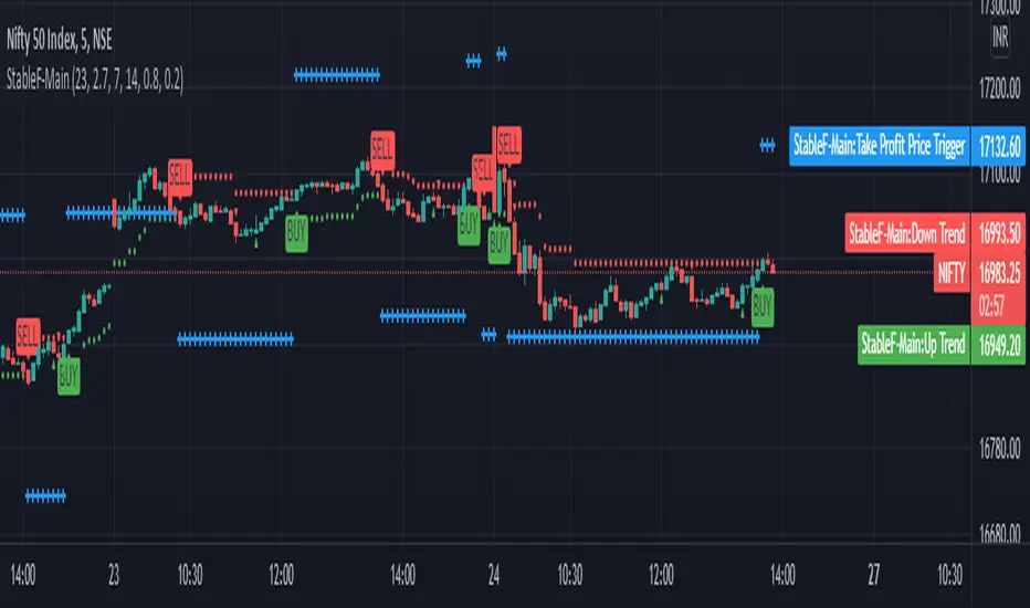
StableF-MainIt is combination of Built in Super trend and Adx with take profit
uptrend is considered when +dmi is above -dmi and +dmi is above 25 and adx is above 25 and supertrend gives Buy
downtrend is considered when -dmi is above +dmi and -dmi is above 25 and adx is above 25 and supertrend give sell
use fibo for target by taking as previous swing high and swing low
-supertrend crossover is referred as buy plotshape
-supertrend cross under is referred as Sell plotshape
-keep stoploss at dot line of supertrend
-adx-dmi crossover (+dmi crossed above -dmi) is shown by Triangle Up symbol
-adx-dmi crossunder( -dmi crosses below +dmi) is shown by Triangle down symbol
--Cross symbol with blue line with linewidth 2 is referred as Take profit
--combine this with adx -dmi setting with 7 and 14
----disclaimer-----
used free built in supertrend and adx so u can use same setting in other broker or in trading view
not responsible for any loss or gain
-only for educational purpose
Market Traffic Light (redesigned)redesigned the market traffic light from funcharts, all honor to him, I just put a new design ;-) and some bugfixes
1. Section (Fear & Greed)
Approximation of the CNN Money Fear & Greed index based on code of user MagicEins. The index shows values between 0 (extreme fear, red) and 100 (extreme greed, green).
2. Section (warning signs)
VIX: Values above 20 are red and below green. The legend shows the value of the current bar including the change from the bar before. The average VIX is about 16. Values over 20 are a sign of stressed market.
Distribution days: A distribution day (loss to the day before > 0,2 % and higher volume ) is marked with a yellow dot. In case there are more than four distributions days within 25 markets days the dot is orange. When big players redistribute their investments distribution days can occur. If this is done often (more than four times within 25 market days) it is possible that the markets changes or that a sector rotation occurs. For calculation distribution days futures of S&P 500 ( ES1! ) and NASDAQ ( NQ1! ) are used because the volume for this calculation is needed. TradingView does not support volumes for S&P 500 or NASDAQ directly.
Markets: A green/red dot signals that the market is above/below its 25-Daily-EMA. A green/red square signals that the market is above/below its 25-Weekly-EMA. Markets can give as a feeling about where investors store their money. E.g. when markets are falling but DUX (Down Jones Utility Average) is rising this means that investors put their money into save haven. This can be a sign that the markets will fall more.
3. Section (panic signs, = signs of reaching a low within a correction of a crash)
VIX-Reversion: A VIX reversion day ( VIX > 20 & VIX high > VIX high of the day before & VIX high – VIX close > 3) is marked as a yellow dot
VVIX: A value equal or above 140 is marked with a yellow dot and shows absolute panic.
PCR Intra max: A value equal or above 1.4 is marked with a yellow dot.
New high/lows: New highs/lows are shown for AMEX, NYSE and NASDAQ. A yellow dot is shown if the ratio is less or equal than 0. 01 .
Down-Day: Down days are shown for AMEX, NYSE and NASDA. A yellow dot is shown if at least 90 % of the whole volume (up and down) is a down volume .
In Addition to the warning signs in the second section a check of the Advance Decline Line (NYSE and NASDAQ) for bullish and bearish divergences is useful. The whole set-up can be seen in the screenshot.
Only one signal normally does not give us a good prediction. Therefore we need to see these indication as a bundle. TradingView gives us the opportunity to check some striking market situations in the past. So feel free to test this indication for building up your own opinion.
Please feel free to comment in case of failures, improvements or experiences (good or bad).

ADX / RSI Strategy by Trade Rush (created by SirPoggy) This is one of many new strategies coming soon which were seen on Trade Rush
This one is the ADX / RSI Strategy seen here:
https:www.youtube.com/watch?v=uSkGE0ujyn4
While the strategy has been modified slightly to use the DMI instead of the ADX, the core of the strategy is essentially the same
Long signals are generated when the RSI is above 70, close is above the 200EMA, and the ADX is above 25 (added is the plus DMI over 25 and minus DMI below 20)
Stop loss is placed below /above the 21 EMA, however, there is a deviation required to ensure price is not too close to where a stop loss would be placed.
Short signals are generated when the RSI is below 30, close is below the 200EMA, and the ADX is above 25 (added is the minus DMI over 25 and plus DMI below 20)
I do not recommend using this strategy but I have provided this code for educational purposes.
Thanks!
Let me know which strategy you'd like coded next in the comments below.

[kai]Futility RatioAn indicator that measures movement inefficiency
Inefficient movement, that is, the range market becomes a high number, the limit is reached at about 60 and a trend occurs
When the range breaks and a trend occurs, the inefficiency drops to about 40 and many trends end.
The full-scale trend goes down further and goes down to about 25, which is evaluated as an efficient movement, the limit is reached and the trend ends.
As for how to use this Inge, the direction of the trend needs to be considered in other ways.
Create a position when you reach 60
Position closed or contrarian at 40 or 25
I assume the usage
動きの非効率性を測定するインジケーターです
非効率な動きをするつまりレンジ相場は高い数字になって、60程度で限界が訪れてトレンドが発生します
レンジがブレイクしトレンドが発生すると40程度まで非効率性は下がりって多くのトレンドは終了します
本格的なトレンドはさらに下がっていって効率的な動きと評価される25程度まで下がって限界が訪れてトレンドが終了します
このインジの使い方はトレンドの方向は他の方法で考える必要がありますが
60まで上がったときにポジション作成
40又は25でポジションクローズ又は逆張り
という使い方を想定しています

Market Traffic LightThis indicator visualizes warning and panic signs, which are shown separately.
1. Section (Fear & Greed)
Approximation of the CNN Money Fear & Greed index based on code of user MagicEins. The index shows values between 0 (extreme fear, red) and 100 (extreme greed, green).
2. Section (warning signs)
VIX: Values above 20 are red and below green. The legend shows the value of the current bar including the change from the bar before. The average VIX is about 16. Values over 20 are a sign of stressed market.
Distribution days: A distribution day (loss to the day before > 0,2 % and higher volume) is marked with a yellow dot. In case there are more than four distributions days within 25 markets days the dot is orange. When big players redistribute their investments distribution days can occur. If this is done often (more than four times within 25 market days) it is possible that the markets changes or that a sector rotation occurs. For calculation distribution days futures of S&P 500 (ES1!) and NASDAQ (NQ1!) are used because the volume for this calculation is needed. TradingView does not support volumes for S&P 500 or NASDAQ directly.
Markets: A green/red dot signals that the market is above/below its 25-Daily-EMA. A green/red square signals that the market is above/below its 25-Weekly-EMA. Markets can give as a feeling about where investors store their money. E.g. when markets are falling but DUX (Down Jones Utility Average) is rising this means that investors put their money into save haven. This can be a sign that the markets will fall more.
3. Section (panic signs, = signs of reaching a low within a correction of a crash)
VIX-Reversion: A VIX reversion day (VIX > 20 & VIX high > VIX high of the day before & VIX high – VIX close > 3) is marked as a yellow dot
VVIX: A value equal or above 140 is marked with a yellow dot and shows absolute panic.
PCR Intra max: A value equal or above 1.4 is marked with a yellow dot.
New high/lows: New highs/lows are shown for AMEX, NYSE and NASDAQ. A yellow dot is shown if the ratio is less or equal than 0.01.
Down-Day: Down days are shown for AMEX, NYSE and NASDA. A yellow dot is shown if at least 90 % of the whole volume (up and down) is a down volume.
In Addition to the warning signs in the second section a check of the Advance Decline Line (NYSE and NASDAQ) for bullish and bearish divergences is useful. The whole set-up can be seen in the screenshot.
Only one signal normally does not give us a good prediction. Therefore we need to see these indication as a bundle. TradingView gives us the opportunity to check some striking market situations in the past. So feel free to test this indication for building up your own opinion.
Please feel free to comment in case of failures, improvements or experiences (good or bad).

Adaptive Trend Navigator [ATH Filter & Risk Engine]Description:
This strategy implements a systematic Trend Following approach designed to capture major moves while actively protecting capital during severe bear markets. It combines a classic Moving Average "Fan" logic with two advanced risk management layers: a 4-Stage Dynamic Stop Loss and a macro-economic "Circuit Breaker" filter.
Core Concepts:
1. Trend Identification (Entry Logic) The script uses a cascade of Simple Moving Averages (SMA 25, 50, 100, 200) to identify the maturity of a trend.
Entries are triggered by specific crossovers (e.g., SMA 25 crossing SMA 50) or by breaking above the previous trade's high ("High-Water Mark" Re-Entry).
2. The "Circuit Breaker" (Crash Protection) To prevent trading during historical market collapses (like 2000 or 2008), the strategy monitors the Nasdaq 100 (QQQ) as a global benchmark:
Normal Regime: If the market is within 20% of its All-Time High, the strategy operates normally.
Crisis Regime: If the QQQ falls more than 20% from its ATH, the "Circuit Breaker" activates (Visualized by a Red Background).
Recovery Rule: In a Crisis Regime, new long positions are blocked unless the QQQ reclaims its SMA 200. This filters out "bull traps" in secular bear markets.
3. 4-Stage Risk Engine (Exit Logic) Once in a trade, the risk management adapts to the position's performance:
Stage 1: Fixed initial Stop Loss (default 10%) for breathing room.
Stage 2: Moves to Break-Even area once the price rises 12%.
Stage 3: Tightens to a trailing stop (8%) after 25% profit.
Stage 4: Maximizes gains with a tight trailing stop (5%) during parabolic moves (>40% profit).
Visual Guide:
SMAs: 25/50/100/200 period lines for trend visualization.
Red Background: Indicates the "Crisis Regime" where trading is halted due to broad market weakness.
Blue Background: Indicates a "Recovery Phase" (Crisis is active, but market is above SMA 200).
Red Line: Shows the dynamic Stop Loss level for active positions.
Settings: All parameters (SMA lengths, Drawdown threshold, Risk Stages) are fully customizable. The QQQ benchmark ticker can also be changed to SPY or other indices depending on the asset class traded.

Dynamic Ratchet Trend Strategy [VIX Filter]Overview This strategy is a long-only trend-following system designed to capture major market moves while strictly managing downside risk through a state-machine based "Ratchet" exit logic. It incorporates a volatility filter using the CBOE VIX index to stay out of (or exit) the market during high-stress environments.
Key Features
1. Multi-Condition Entries The strategy looks for momentum shifts and trend breakouts using four Simple Moving Averages (25, 50, 100, 200).
Momentum Cross: SMA 25 crossover above SMA 50.
Trend Breakouts: A specific "3-Bar Breakout" logic above the SMA 50, 100, or 200. This requires the price to hold above the SMA for 3 consecutive bars after being below it, reducing false signals compared to simple closes.
2. VIX Volatility Filter Before entering any trade, the script checks the CBOE:VIX.
Filter: If VIX is above the threshold (default 32), new entries are blocked.
Panic Exit: If you are in a position and the VIX spikes above the threshold, the strategy executes an immediate "Panic Exit" to preserve capital during market crashes.
3. The "Ratchet" Exit System (3 Stages) Unlike a standard trailing stop, this strategy uses a 3-stage dynamic exit mechanism that tightens as profits grow:
Stage 0 (Initial Risk): Standard percentage-based Stop Loss from the entry price.
Stage 1 (The Lock-In): Triggered when profit hits 10% (configurable).
Unique Logic: Instead of trailing from the highest high, the stop is calculated based on the price at the exact moment this stage was triggered. It "steps up" once and holds, securing the initial move without being prematurely stopped out by normal volatility.
Stage 2 (Trailing Mode): Triggered when profit hits 15% (configurable).
The strategy switches to a classic Trailing Stop, following the percentage distance from the Highest High.
4. Emergency Backup A "Dead Cross" (SMA 25 crossing under SMA 50) acts as a final fail-safe to close positions if the trend reverses completely before hitting a stop.
Settings & Inputs
SMAs: Customize the lengths for all four moving averages.
VIX Filter: Toggle the filter on/off and set the panic threshold.
Exit Logic: Fully customizable percentages for Initial SL, Stage 1 Trigger/Distance, and Stage 2 Trigger/Trailing Distance.
Disclaimer This script is for educational purposes only. Past performance is not indicative of future results. Always manage your risk appropriately.

لbsm15// This work is licensed under a Attribution-NonCommercial-ShareAlike 4.0 International (CC BY-NC-SA 4.0) creativecommons.org
// © LuxAlgo
//@version=5
indicator("لbsm15", overlay = true, max_lines_count = 500, max_boxes_count = 500, max_bars_back = 3000)
//------------------------------------------------------------------------------
//Settings
//-----------------------------------------------------------------------------{
liqGrp = 'Liquidity Detection'
liqLen = input.int (7, title = 'Detection Length', minval = 3, maxval = 13, inline = 'LIQ', group = liqGrp)
liqMar = 10 / input.float (6.9, 'Margin', minval = 4, maxval = 9, step = 0.1, inline = 'LIQ', group = liqGrp)
liqBuy = input.bool (true, 'Buyside Liquidity Zones, Margin', inline = 'Buyside', group = liqGrp)
marBuy = input.float(2.3, '', minval = 1.5, maxval = 10, step = .1, inline = 'Buyside', group = liqGrp)
cLIQ_B = input.color (color.new(#4caf50, 0), '', inline = 'Buyside', group = liqGrp)
liqSel = input.bool (true, 'Sellside Liquidity Zones, Margin', inline = 'Sellside', group = liqGrp)
marSel = input.float(2.3, '', minval = 1.5, maxval = 10, step = .1, inline = 'Sellside', group = liqGrp)
cLIQ_S = input.color (color.new(#f23645, 0), '', inline = 'Sellside', group = liqGrp)
lqVoid = input.bool (false, 'Liquidity Voids, Bullish', inline = 'void', group = liqGrp)
cLQV_B = input.color (color.new(#4caf50, 0), '', inline = 'void', group = liqGrp)
cLQV_S = input.color (color.new(#f23645, 0), 'Bearish', inline = 'void', group = liqGrp)
lqText = input.bool (false, 'Label', inline = 'void', group = liqGrp)
mode = input.string('Present', title = 'Mode', options = , inline = 'MOD', group = liqGrp)
visLiq = input.int (3, ' # Visible Levels', minval = 1, maxval = 50, inline = 'MOD', group = liqGrp)
//-----------------------------------------------------------------------------}
//General Calculations
//-----------------------------------------------------------------------------{
maxSize = 50
atr = ta.atr(10)
atr200 = ta.atr(200)
per = mode == 'Present' ? last_bar_index - bar_index <= 500 : true
//-----------------------------------------------------------------------------}
//User Defined Types
//-----------------------------------------------------------------------------{
// @type used to store pivot high/low data
//
// @field d (array) The array where the trend direction is to be maintained
// @field x (array) The array where the bar index value of pivot high/low is to be maintained
// @field y (array) The array where the price value of pivot high/low is to be maintained
type ZZ
int d
int x
float y
// @type bar properties with their values
//
// @field o (float) open price of the bar
// @field h (float) high price of the bar
// @field l (float) low price of the bar
// @field c (float) close price of the bar
// @field i (int) index of the bar
type bar
float o = open
float h = high
float l = low
float c = close
int i = bar_index
// @type liquidity object definition
//
// @field bx (box) box maitaing the liquity level margin extreme levels
// @field bxz (box) box maitaing the liquity zone margin extreme levels
// @field bxt (box) box maitaing the labels
// @field brZ (bool) mainains broken zone status
// @field brL (bool) mainains broken level status
// @field ln (line) maitaing the liquity level line
// @field lne (line) maitaing the liquity extended level line
type liq
box bx
box bxz
box bxt
bool brZ
bool brL
line ln
line lne
//-----------------------------------------------------------------------------}
//Variables
//-----------------------------------------------------------------------------{
var ZZ aZZ = ZZ.new(
array.new (maxSize, 0),
array.new (maxSize, 0),
array.new (maxSize, na)
)
bar b = bar.new()
var liq b_liq_B = array.new (1, liq.new(box(na), box(na), box(na), false, false, line(na), line(na)))
var liq b_liq_S = array.new (1, liq.new(box(na), box(na), box(na), false, false, line(na), line(na)))
var b_liq_V = array.new_box()
var int dir = na, var int x1 = na, var float y1 = na, var int x2 = na, var float y2 = na
//-----------------------------------------------------------------------------}
//Functions/methods
//-----------------------------------------------------------------------------{
// @function maintains arrays
// it prepends a `value` to the arrays and removes their oldest element at last position
// @param aZZ (UDT, array, array>) The UDT obejct of arrays
// @param _d (array) The array where the trend direction is maintained
// @param _x (array) The array where the bar index value of pivot high/low is maintained
// @param _y (array) The array where the price value of pivot high/low is maintained
//
// @returns none
method in_out(ZZ aZZ, int _d, int _x, float _y) =>
aZZ.d.unshift(_d), aZZ.x.unshift(_x), aZZ.y.unshift(_y), aZZ.d.pop(), aZZ.x.pop(), aZZ.y.pop()
// @function (build-in) sets the maximum number of bars that is available for historical reference
max_bars_back(time, 1000)
//-----------------------------------------------------------------------------}
//Calculations
//-----------------------------------------------------------------------------{
x2 := b.i - 1
ph = ta.pivothigh(liqLen, 1)
pl = ta.pivotlow (liqLen, 1)
if ph
dir := aZZ.d.get(0)
x1 := aZZ.x.get(0)
y1 := aZZ.y.get(0)
y2 := nz(b.h )
if dir < 1
aZZ.in_out(1, x2, y2)
else
if dir == 1 and ph > y1
aZZ.x.set(0, x2), aZZ.y.set(0, y2)
if per
count = 0
st_P = 0.
st_B = 0
minP = 0.
maxP = 10e6
for i = 0 to maxSize - 1
if aZZ.d.get(i) == 1
if aZZ.y.get(i) > ph + (atr / liqMar)
break
else
if aZZ.y.get(i) > ph - (atr / liqMar) and aZZ.y.get(i) < ph + (atr / liqMar)
count += 1
st_B := aZZ.x.get(i)
st_P := aZZ.y.get(i)
if aZZ.y.get(i) > minP
minP := aZZ.y.get(i)
if aZZ.y.get(i) < maxP
maxP := aZZ.y.get(i)
if count > 2
getB = b_liq_B.get(0)
if st_B == getB.bx.get_left()
getB.bx.set_top(math.avg(minP, maxP) + (atr / liqMar))
getB.bx.set_rightbottom(b.i + 10, math.avg(minP, maxP) - (atr / liqMar))
else
b_liq_B.unshift(
liq.new(
box.new(st_B, math.avg(minP, maxP) + (atr / liqMar), b.i + 10, math.avg(minP, maxP) - (atr / liqMar), bgcolor=color(na), border_color=color(na)),
box.new(na, na, na, na, bgcolor = color(na), border_color = color(na)),
box.new(st_B, st_P, b.i + 10, st_P, text = 'Buyside liquidity', text_size = size.tiny, text_halign = text.align_left, text_valign = text.align_bottom, text_color = color.new(cLIQ_B, 25), bgcolor = color(na), border_color = color(na)),
false,
false,
line.new(st_B , st_P, b.i - 1, st_P, color = color.new(cLIQ_B, 0)),
line.new(b.i - 1, st_P, na , st_P, color = color.new(cLIQ_B, 0), style = line.style_dotted))
)
alert('buyside liquidity level detected/updated for ' + syminfo.ticker)
if b_liq_B.size() > visLiq
getLast = b_liq_B.pop()
getLast.bx.delete()
getLast.bxz.delete()
getLast.bxt.delete()
getLast.ln.delete()
getLast.lne.delete()
if pl
dir := aZZ.d.get (0)
x1 := aZZ.x.get (0)
y1 := aZZ.y.get (0)
y2 := nz(b.l )
if dir > -1
aZZ.in_out(-1, x2, y2)
else
if dir == -1 and pl < y1
aZZ.x.set(0, x2), aZZ.y.set(0, y2)
if per
count = 0
st_P = 0.
st_B = 0
minP = 0.
maxP = 10e6
for i = 0 to maxSize - 1
if aZZ.d.get(i) == -1
if aZZ.y.get(i) < pl - (atr / liqMar)
break
else
if aZZ.y.get(i) > pl - (atr / liqMar) and aZZ.y.get(i) < pl + (atr / liqMar)
count += 1
st_B := aZZ.x.get(i)
st_P := aZZ.y.get(i)
if aZZ.y.get(i) > minP
minP := aZZ.y.get(i)
if aZZ.y.get(i) < maxP
maxP := aZZ.y.get(i)
if count > 2
getB = b_liq_S.get(0)
if st_B == getB.bx.get_left()
getB.bx.set_top(math.avg(minP, maxP) + (atr / liqMar))
getB.bx.set_rightbottom(b.i + 10, math.avg(minP, maxP) - (atr / liqMar))
else
b_liq_S.unshift(
liq.new(
box.new(st_B, math.avg(minP, maxP) + (atr / liqMar), b.i + 10, math.avg(minP, maxP) - (atr / liqMar), bgcolor=color(na), border_color=color(na)),
box.new(na, na, na, na, bgcolor=color(na), border_color=color(na)),
box.new(st_B, st_P, b.i + 10, st_P, text = 'Sellside liquidity', text_size = size.tiny, text_halign = text.align_left, text_valign = text.align_top, text_color = color.new(cLIQ_S, 25), bgcolor=color(na), border_color=color(na)),
false,
false,
line.new(st_B , st_P, b.i - 1, st_P, color = color.new(cLIQ_S, 0)),
line.new(b.i - 1, st_P, na , st_P, color = color.new(cLIQ_S, 0), style = line.style_dotted))
)
alert('sellside liquidity level detected/updated for ' + syminfo.ticker)
if b_liq_S.size() > visLiq
getLast = b_liq_S.pop()
getLast.bx.delete()
getLast.bxz.delete()
getLast.bxt.delete()
getLast.ln.delete()
getLast.lne.delete()
for i = 0 to b_liq_B.size() - 1
x = b_liq_B.get(i)
if not x.brL
x.lne.set_x2(b.i)
if b.h > x.bx.get_top()
x.brL := true
x.brZ := true
alert('buyside liquidity level breached for ' + syminfo.ticker)
x.bxz.set_lefttop(b.i - 1, math.min(x.ln.get_y1() + marBuy * (atr), b.h))
x.bxz.set_rightbottom(b.i + 1, x.ln.get_y1())
x.bxz.set_bgcolor(color.new(cLIQ_B, liqBuy ? 73 : 100))
else if x.brZ
if b.l > x.ln.get_y1() - marBuy * (atr) and b.h < x.ln.get_y1() + marBuy * (atr)
x.bxz.set_right(b.i + 1)
x.bxz.set_top(math.max(b.h, x.bxz.get_top()))
if liqBuy
x.lne.set_x2(b.i + 1)
else
x.brZ := false
for i = 0 to b_liq_S.size() - 1
x = b_liq_S.get(i)
if not x.brL
x.lne.set_x2(b.i)
if b.l < x.bx.get_bottom()
x.brL := true
x.brZ := true
alert('sellside liquidity level breached for ' + syminfo.ticker)
x.bxz.set_lefttop(b.i - 1, x.ln.get_y1())
x.bxz.set_rightbottom(b.i + 1, math.max(x.ln.get_y1() - marSel * (atr), b.l))
x.bxz.set_bgcolor(color.new(cLIQ_S, liqSel ? 73 : 100))
else if x.brZ
if b.l > x.ln.get_y1() - marSel * (atr) and b.h < x.ln.get_y1() + marSel * (atr)
x.bxz.set_rightbottom(b.i + 1, math.min(b.l, x.bxz.get_bottom()))
if liqSel
x.lne.set_x2(b.i + 1)
else
x.brZ := false
if lqVoid and per
bull = b.l - b.h > atr200 and b.l > b.h and b.c > b.h
bear = b.l - b.h > atr200 and b.h < b.l and b.c < b.l
if bull
l = 13
if bull
st = math.abs(b.l - b.l ) / l
for i = 0 to l - 1
array.push(b_liq_V, box.new(b.i - 2, b.l + i * st, b.i, b.l + (i + 1) * st, border_color = na, bgcolor = color.new(cLQV_B, 90) ))
else
st = math.abs(b.l - b.h ) / l
for i = 0 to l - 1
if lqText and i == 0
array.push(b_liq_V, box.new(b.i - 2, b.h + i * st, b.i, b.h + (i + 1) * st, text = 'Liquidity Void ', text_size = size.tiny, text_halign = text.align_right, text_valign = text.align_bottom, text_color = na, border_color = na, bgcolor = color.new(cLQV_B, 90) ))
else
array.push(b_liq_V, box.new(b.i - 2, b.h + i * st, b.i, b.h + (i + 1) * st, border_color = na, bgcolor = color.new(cLQV_B, 90) ))
if bear
l = 13
if bear
st = math.abs(b.h - b.h) / l
for i = 0 to l - 1
array.push(b_liq_V, box.new(b.i - 2, b.h + i * st, b.i, b.h + (i + 1) * st, border_color = na, bgcolor = color.new(cLQV_S, 90) ))
else
st = math.abs(b.l - b.h) / l
for i = 0 to l - 1
if lqText and i == l - 1
array.push(b_liq_V, box.new(b.i - 2, b.h + i * st, b.i, b.h + (i + 1) * st, text = 'Liquidity Void ', text_size = size.tiny, text_halign = text.align_right, text_valign = text.align_top, text_color = na, border_color = na, bgcolor = color.new(cLQV_S, 90) ))
else
array.push(b_liq_V, box.new(b.i - 2, b.h + i * st, b.i, b.h + (i + 1) * st, border_color = na, bgcolor = color.new(cLQV_S, 90) ))
if b_liq_V.size() > 0
qt = b_liq_V.size()
for bn = qt - 1 to 0
if bn < b_liq_V.size()
cb = b_liq_V.get(bn)
ba = math.avg(cb.get_bottom(), cb.get_top())
if math.sign(b.c - ba) != math.sign(b.c - ba) or math.sign(b.c - ba) != math.sign(b.l - ba) or math.sign(b.c - ba) != math.sign(b.h - ba)
b_liq_V.remove(bn)
else
cb.set_right(b.i + 1)
if b.i - cb.get_left() > 21
cb.set_text_color(color.new(color.gray, 25))
//-----------------------------------------------------------------------------}

Dimensional Resonance ProtocolDimensional Resonance Protocol
🌀 CORE INNOVATION: PHASE SPACE RECONSTRUCTION & EMERGENCE DETECTION
The Dimensional Resonance Protocol represents a paradigm shift from traditional technical analysis to complexity science. Rather than measuring price levels or indicator crossovers, DRP reconstructs the hidden attractor governing market dynamics using Takens' embedding theorem, then detects emergence —the rare moments when multiple dimensions of market behavior spontaneously synchronize into coherent, predictable states.
The Complexity Hypothesis:
Markets are not simple oscillators or random walks—they are complex adaptive systems existing in high-dimensional phase space. Traditional indicators see only shadows (one-dimensional projections) of this higher-dimensional reality. DRP reconstructs the full phase space using time-delay embedding, revealing the true structure of market dynamics.
Takens' Embedding Theorem (1981):
A profound mathematical result from dynamical systems theory: Given a time series from a complex system, we can reconstruct its full phase space by creating delayed copies of the observation.
Mathematical Foundation:
From single observable x(t), create embedding vectors:
X(t) =
Where:
• d = Embedding dimension (default 5)
• τ = Time delay (default 3 bars)
• x(t) = Price or return at time t
Key Insight: If d ≥ 2D+1 (where D is the true attractor dimension), this embedding is topologically equivalent to the actual system dynamics. We've reconstructed the hidden attractor from a single price series.
Why This Matters:
Markets appear random in one dimension (price chart). But in reconstructed phase space, structure emerges—attractors, limit cycles, strange attractors. When we identify these structures, we can detect:
• Stable regions : Predictable behavior (trade opportunities)
• Chaotic regions : Unpredictable behavior (avoid trading)
• Critical transitions : Phase changes between regimes
Phase Space Magnitude Calculation:
phase_magnitude = sqrt(Σ ² for i = 0 to d-1)
This measures the "energy" or "momentum" of the market trajectory through phase space. High magnitude = strong directional move. Low magnitude = consolidation.
📊 RECURRENCE QUANTIFICATION ANALYSIS (RQA)
Once phase space is reconstructed, we analyze its recurrence structure —when does the system return near previous states?
Recurrence Plot Foundation:
A recurrence occurs when two phase space points are closer than threshold ε:
R(i,j) = 1 if ||X(i) - X(j)|| < ε, else 0
This creates a binary matrix showing when the system revisits similar states.
Key RQA Metrics:
1. Recurrence Rate (RR):
RR = (Number of recurrent points) / (Total possible pairs)
• RR near 0: System never repeats (highly stochastic)
• RR = 0.1-0.3: Moderate recurrence (tradeable patterns)
• RR > 0.5: System stuck in attractor (ranging market)
• RR near 1: System frozen (no dynamics)
Interpretation: Moderate recurrence is optimal —patterns exist but market isn't stuck.
2. Determinism (DET):
Measures what fraction of recurrences form diagonal structures in the recurrence plot. Diagonals indicate deterministic evolution (trajectory follows predictable paths).
DET = (Recurrence points on diagonals) / (Total recurrence points)
• DET < 0.3: Random dynamics
• DET = 0.3-0.7: Moderate determinism (patterns with noise)
• DET > 0.7: Strong determinism (technical patterns reliable)
Trading Implication: Signals are prioritized when DET > 0.3 (deterministic state) and RR is moderate (not stuck).
Threshold Selection (ε):
Default ε = 0.10 × std_dev means two states are "recurrent" if within 10% of a standard deviation. This is tight enough to require genuine similarity but loose enough to find patterns.
🔬 PERMUTATION ENTROPY: COMPLEXITY MEASUREMENT
Permutation entropy measures the complexity of a time series by analyzing the distribution of ordinal patterns.
Algorithm (Bandt & Pompe, 2002):
1. Take overlapping windows of length n (default n=4)
2. For each window, record the rank order pattern
Example: → pattern (ranks from lowest to highest)
3. Count frequency of each possible pattern
4. Calculate Shannon entropy of pattern distribution
Mathematical Formula:
H_perm = -Σ p(π) · ln(p(π))
Where π ranges over all n! possible permutations, p(π) is the probability of pattern π.
Normalized to :
H_norm = H_perm / ln(n!)
Interpretation:
• H < 0.3 : Very ordered, crystalline structure (strong trending)
• H = 0.3-0.5 : Ordered regime (tradeable with patterns)
• H = 0.5-0.7 : Moderate complexity (mixed conditions)
• H = 0.7-0.85 : Complex dynamics (challenging to trade)
• H > 0.85 : Maximum entropy (nearly random, avoid)
Entropy Regime Classification:
DRP classifies markets into five entropy regimes:
• CRYSTALLINE (H < 0.3): Maximum order, persistent trends
• ORDERED (H < 0.5): Clear patterns, momentum strategies work
• MODERATE (H < 0.7): Mixed dynamics, adaptive required
• COMPLEX (H < 0.85): High entropy, mean reversion better
• CHAOTIC (H ≥ 0.85): Near-random, minimize trading
Why Permutation Entropy?
Unlike traditional entropy methods requiring binning continuous data (losing information), permutation entropy:
• Works directly on time series
• Robust to monotonic transformations
• Computationally efficient
• Captures temporal structure, not just distribution
• Immune to outliers (uses ranks, not values)
⚡ LYAPUNOV EXPONENT: CHAOS vs STABILITY
The Lyapunov exponent λ measures sensitivity to initial conditions —the hallmark of chaos.
Physical Meaning:
Two trajectories starting infinitely close will diverge at exponential rate e^(λt):
Distance(t) ≈ Distance(0) × e^(λt)
Interpretation:
• λ > 0 : Positive Lyapunov exponent = CHAOS
- Small errors grow exponentially
- Long-term prediction impossible
- System is sensitive, unpredictable
- AVOID TRADING
• λ ≈ 0 : Near-zero = CRITICAL STATE
- Edge of chaos
- Transition zone between order and disorder
- Moderate predictability
- PROCEED WITH CAUTION
• λ < 0 : Negative Lyapunov exponent = STABLE
- Small errors decay
- Trajectories converge
- System is predictable
- OPTIMAL FOR TRADING
Estimation Method:
DRP estimates λ by tracking how quickly nearby states diverge over a rolling window (default 20 bars):
For each bar i in window:
δ₀ = |x - x | (initial separation)
δ₁ = |x - x | (previous separation)
if δ₁ > 0:
ratio = δ₀ / δ₁
log_ratios += ln(ratio)
λ ≈ average(log_ratios)
Stability Classification:
• STABLE : λ < 0 (negative growth rate)
• CRITICAL : |λ| < 0.1 (near neutral)
• CHAOTIC : λ > 0.2 (strong positive growth)
Signal Filtering:
By default, NEXUS requires λ < 0 (stable regime) for signal confirmation. This filters out trades during chaotic periods when technical patterns break down.
📐 HIGUCHI FRACTAL DIMENSION
Fractal dimension measures self-similarity and complexity of the price trajectory.
Theoretical Background:
A curve's fractal dimension D ranges from 1 (smooth line) to 2 (space-filling curve):
• D ≈ 1.0 : Smooth, persistent trending
• D ≈ 1.5 : Random walk (Brownian motion)
• D ≈ 2.0 : Highly irregular, space-filling
Higuchi Method (1988):
For a time series of length N, construct k different curves by taking every k-th point:
L(k) = (1/k) × Σ|x - x | × (N-1)/(⌊(N-m)/k⌋ × k)
For different values of k (1 to k_max), calculate L(k). The fractal dimension is the slope of log(L(k)) vs log(1/k):
D = slope of log(L) vs log(1/k)
Market Interpretation:
• D < 1.35 : Strong trending, persistent (Hurst > 0.5)
- TRENDING regime
- Momentum strategies favored
- Breakouts likely to continue
• D = 1.35-1.45 : Moderate persistence
- PERSISTENT regime
- Trend-following with caution
- Patterns have meaning
• D = 1.45-1.55 : Random walk territory
- RANDOM regime
- Efficiency hypothesis holds
- Technical analysis least reliable
• D = 1.55-1.65 : Anti-persistent (mean-reverting)
- ANTI-PERSISTENT regime
- Oscillator strategies work
- Overbought/oversold meaningful
• D > 1.65 : Highly complex, choppy
- COMPLEX regime
- Avoid directional bets
- Wait for regime change
Signal Filtering:
Resonance signals (secondary signal type) require D < 1.5, indicating trending or persistent dynamics where momentum has meaning.
🔗 TRANSFER ENTROPY: CAUSAL INFORMATION FLOW
Transfer entropy measures directed causal influence between time series—not just correlation, but actual information transfer.
Schreiber's Definition (2000):
Transfer entropy from X to Y measures how much knowing X's past reduces uncertainty about Y's future:
TE(X→Y) = H(Y_future | Y_past) - H(Y_future | Y_past, X_past)
Where H is Shannon entropy.
Key Properties:
1. Directional : TE(X→Y) ≠ TE(Y→X) in general
2. Non-linear : Detects complex causal relationships
3. Model-free : No assumptions about functional form
4. Lag-independent : Captures delayed causal effects
Three Causal Flows Measured:
1. Volume → Price (TE_V→P):
Measures how much volume patterns predict price changes.
• TE > 0 : Volume provides predictive information about price
- Institutional participation driving moves
- Volume confirms direction
- High reliability
• TE ≈ 0 : No causal flow (weak volume/price relationship)
- Volume uninformative
- Caution on signals
• TE < 0 (rare): Suggests price leading volume
- Potentially manipulated or thin market
2. Volatility → Momentum (TE_σ→M):
Does volatility expansion predict momentum changes?
• Positive TE : Volatility precedes momentum shifts
- Breakout dynamics
- Regime transitions
3. Structure → Price (TE_S→P):
Do support/resistance patterns causally influence price?
• Positive TE : Structural levels have causal impact
- Technical levels matter
- Market respects structure
Net Causal Flow:
Net_Flow = TE_V→P + 0.5·TE_σ→M + TE_S→P
• Net > +0.1 : Bullish causal structure
• Net < -0.1 : Bearish causal structure
• |Net| < 0.1 : Neutral/unclear causation
Causal Gate:
For signal confirmation, NEXUS requires:
• Buy signals : TE_V→P > 0 AND Net_Flow > 0.05
• Sell signals : TE_V→P > 0 AND Net_Flow < -0.05
This ensures volume is actually driving price (causal support exists), not just correlated noise.
Implementation Note:
Computing true transfer entropy requires discretizing continuous data into bins (default 6 bins) and estimating joint probability distributions. NEXUS uses a hybrid approach combining TE theory with autocorrelation structure and lagged cross-correlation to approximate information transfer in computationally efficient manner.
🌊 HILBERT PHASE COHERENCE
Phase coherence measures synchronization across market dimensions using Hilbert transform analysis.
Hilbert Transform Theory:
For a signal x(t), the Hilbert transform H (t) creates an analytic signal:
z(t) = x(t) + i·H (t) = A(t)·e^(iφ(t))
Where:
• A(t) = Instantaneous amplitude
• φ(t) = Instantaneous phase
Instantaneous Phase:
φ(t) = arctan(H (t) / x(t))
The phase represents where the signal is in its natural cycle—analogous to position on a unit circle.
Four Dimensions Analyzed:
1. Momentum Phase : Phase of price rate-of-change
2. Volume Phase : Phase of volume intensity
3. Volatility Phase : Phase of ATR cycles
4. Structure Phase : Phase of position within range
Phase Locking Value (PLV):
For two signals with phases φ₁(t) and φ₂(t), PLV measures phase synchronization:
PLV = |⟨e^(i(φ₁(t) - φ₂(t)))⟩|
Where ⟨·⟩ is time average over window.
Interpretation:
• PLV = 0 : Completely random phase relationship (no synchronization)
• PLV = 0.5 : Moderate phase locking
• PLV = 1 : Perfect synchronization (phases locked)
Pairwise PLV Calculations:
• PLV_momentum-volume : Are momentum and volume cycles synchronized?
• PLV_momentum-structure : Are momentum cycles aligned with structure?
• PLV_volume-structure : Are volume and structural patterns in phase?
Overall Phase Coherence:
Coherence = (PLV_mom-vol + PLV_mom-struct + PLV_vol-struct) / 3
Signal Confirmation:
Emergence signals require coherence ≥ threshold (default 0.70):
• Below 0.70: Dimensions not synchronized, no coherent market state
• Above 0.70: Dimensions in phase, coherent behavior emerging
Coherence Direction:
The summed phase angles indicate whether synchronized dimensions point bullish or bearish:
Direction = sin(φ_momentum) + 0.5·sin(φ_volume) + 0.5·sin(φ_structure)
• Direction > 0 : Phases pointing upward (bullish synchronization)
• Direction < 0 : Phases pointing downward (bearish synchronization)
🌀 EMERGENCE SCORE: MULTI-DIMENSIONAL ALIGNMENT
The emergence score aggregates all complexity metrics into a single 0-1 value representing market coherence.
Eight Components with Weights:
1. Phase Coherence (20%):
Direct contribution: coherence × 0.20
Measures dimensional synchronization.
2. Entropy Regime (15%):
Contribution: (0.6 - H_perm) / 0.6 × 0.15 if H < 0.6, else 0
Rewards low entropy (ordered, predictable states).
3. Lyapunov Stability (12%):
• λ < 0 (stable): +0.12
• |λ| < 0.1 (critical): +0.08
• λ > 0.2 (chaotic): +0.0
Requires stable, predictable dynamics.
4. Fractal Dimension Trending (12%):
Contribution: (1.45 - D) / 0.45 × 0.12 if D < 1.45, else 0
Rewards trending fractal structure (D < 1.45).
5. Dimensional Resonance (12%):
Contribution: |dimensional_resonance| × 0.12
Measures alignment across momentum, volume, structure, volatility dimensions.
6. Causal Flow Strength (9%):
Contribution: |net_causal_flow| × 0.09
Rewards strong causal relationships.
7. Phase Space Embedding (10%):
Contribution: min(|phase_magnitude_norm|, 3.0) / 3.0 × 0.10 if |magnitude| > 1.0
Rewards strong trajectory in reconstructed phase space.
8. Recurrence Quality (10%):
Contribution: determinism × 0.10 if DET > 0.3 AND 0.1 < RR < 0.8
Rewards deterministic patterns with moderate recurrence.
Total Emergence Score:
E = Σ(components) ∈
Capped at 1.0 maximum.
Emergence Direction:
Separate calculation determining bullish vs bearish:
• Dimensional resonance sign
• Net causal flow sign
• Phase magnitude correlation with momentum
Signal Threshold:
Default emergence_threshold = 0.75 means 75% of maximum possible emergence score required to trigger signals.
Why Emergence Matters:
Traditional indicators measure single dimensions. Emergence detects self-organization —when multiple independent dimensions spontaneously align. This is the market equivalent of a phase transition in physics, where microscopic chaos gives way to macroscopic order.
These are the highest-probability trade opportunities because the entire system is resonating in the same direction.
🎯 SIGNAL GENERATION: EMERGENCE vs RESONANCE
DRP generates two tiers of signals with different requirements:
TIER 1: EMERGENCE SIGNALS (Primary)
Requirements:
1. Emergence score ≥ threshold (default 0.75)
2. Phase coherence ≥ threshold (default 0.70)
3. Emergence direction > 0.2 (bullish) or < -0.2 (bearish)
4. Causal gate passed (if enabled): TE_V→P > 0 and net_flow confirms direction
5. Stability zone (if enabled): λ < 0 or |λ| < 0.1
6. Price confirmation: Close > open (bulls) or close < open (bears)
7. Cooldown satisfied: bars_since_signal ≥ cooldown_period
EMERGENCE BUY:
• All above conditions met with bullish direction
• Market has achieved coherent bullish state
• Multiple dimensions synchronized upward
EMERGENCE SELL:
• All above conditions met with bearish direction
• Market has achieved coherent bearish state
• Multiple dimensions synchronized downward
Premium Emergence:
When signal_quality (emergence_score × phase_coherence) > 0.7:
• Displayed as ★ star symbol
• Highest conviction trades
• Maximum dimensional alignment
Standard Emergence:
When signal_quality 0.5-0.7:
• Displayed as ◆ diamond symbol
• Strong signals but not perfect alignment
TIER 2: RESONANCE SIGNALS (Secondary)
Requirements:
1. Dimensional resonance > +0.6 (bullish) or < -0.6 (bearish)
2. Fractal dimension < 1.5 (trending/persistent regime)
3. Price confirmation matches direction
4. NOT in chaotic regime (λ < 0.2)
5. Cooldown satisfied
6. NO emergence signal firing (resonance is fallback)
RESONANCE BUY:
• Dimensional alignment without full emergence
• Trending fractal structure
• Moderate conviction
RESONANCE SELL:
• Dimensional alignment without full emergence
• Bearish resonance with trending structure
• Moderate conviction
Displayed as small ▲/▼ triangles with transparency.
Signal Hierarchy:
IF emergence conditions met:
Fire EMERGENCE signal (★ or ◆)
ELSE IF resonance conditions met:
Fire RESONANCE signal (▲ or ▼)
ELSE:
No signal
Cooldown System:
After any signal fires, cooldown_period (default 5 bars) must elapse before next signal. This prevents signal clustering during persistent conditions.
Cooldown tracks using bar_index:
bars_since_signal = current_bar_index - last_signal_bar_index
cooldown_ok = bars_since_signal >= cooldown_period
🎨 VISUAL SYSTEM: MULTI-LAYER COMPLEXITY
DRP provides rich visual feedback across four distinct layers:
LAYER 1: COHERENCE FIELD (Background)
Colored background intensity based on phase coherence:
• No background : Coherence < 0.5 (incoherent state)
• Faint glow : Coherence 0.5-0.7 (building coherence)
• Stronger glow : Coherence > 0.7 (coherent state)
Color:
• Cyan/teal: Bullish coherence (direction > 0)
• Red/magenta: Bearish coherence (direction < 0)
• Blue: Neutral coherence (direction ≈ 0)
Transparency: 98 minus (coherence_intensity × 10), so higher coherence = more visible.
LAYER 2: STABILITY/CHAOS ZONES
Background color indicating Lyapunov regime:
• Green tint (95% transparent): λ < 0, STABLE zone
- Safe to trade
- Patterns meaningful
• Gold tint (90% transparent): |λ| < 0.1, CRITICAL zone
- Edge of chaos
- Moderate risk
• Red tint (85% transparent): λ > 0.2, CHAOTIC zone
- Avoid trading
- Unpredictable behavior
LAYER 3: DIMENSIONAL RIBBONS
Three EMAs representing dimensional structure:
• Fast ribbon : EMA(8) in cyan/teal (fast dynamics)
• Medium ribbon : EMA(21) in blue (intermediate)
• Slow ribbon : EMA(55) in red/magenta (slow dynamics)
Provides visual reference for multi-scale structure without cluttering with raw phase space data.
LAYER 4: CAUSAL FLOW LINE
A thicker line plotted at EMA(13) colored by net causal flow:
• Cyan/teal : Net_flow > +0.1 (bullish causation)
• Red/magenta : Net_flow < -0.1 (bearish causation)
• Gray : |Net_flow| < 0.1 (neutral causation)
Shows real-time direction of information flow.
EMERGENCE FLASH:
Strong background flash when emergence signals fire:
• Cyan flash for emergence buy
• Red flash for emergence sell
• 80% transparency for visibility without obscuring price
📊 COMPREHENSIVE DASHBOARD
Real-time monitoring of all complexity metrics:
HEADER:
• 🌀 DRP branding with gold accent
CORE METRICS:
EMERGENCE:
• Progress bar (█ filled, ░ empty) showing 0-100%
• Percentage value
• Direction arrow (↗ bull, ↘ bear, → neutral)
• Color-coded: Green/gold if active, gray if low
COHERENCE:
• Progress bar showing phase locking value
• Percentage value
• Checkmark ✓ if ≥ threshold, circle ○ if below
• Color-coded: Cyan if coherent, gray if not
COMPLEXITY SECTION:
ENTROPY:
• Regime name (CRYSTALLINE/ORDERED/MODERATE/COMPLEX/CHAOTIC)
• Numerical value (0.00-1.00)
• Color: Green (ordered), gold (moderate), red (chaotic)
LYAPUNOV:
• State (STABLE/CRITICAL/CHAOTIC)
• Numerical value (typically -0.5 to +0.5)
• Status indicator: ● stable, ◐ critical, ○ chaotic
• Color-coded by state
FRACTAL:
• Regime (TRENDING/PERSISTENT/RANDOM/ANTI-PERSIST/COMPLEX)
• Dimension value (1.0-2.0)
• Color: Cyan (trending), gold (random), red (complex)
PHASE-SPACE:
• State (STRONG/ACTIVE/QUIET)
• Normalized magnitude value
• Parameters display: d=5 τ=3
CAUSAL SECTION:
CAUSAL:
• Direction (BULL/BEAR/NEUTRAL)
• Net flow value
• Flow indicator: →P (to price), P← (from price), ○ (neutral)
V→P:
• Volume-to-price transfer entropy
• Small display showing specific TE value
DIMENSIONAL SECTION:
RESONANCE:
• Progress bar of absolute resonance
• Signed value (-1 to +1)
• Color-coded by direction
RECURRENCE:
• Recurrence rate percentage
• Determinism percentage display
• Color-coded: Green if high quality
STATE SECTION:
STATE:
• Current mode: EMERGENCE / RESONANCE / CHAOS / SCANNING
• Icon: 🚀 (emergence buy), 💫 (emergence sell), ▲ (resonance buy), ▼ (resonance sell), ⚠ (chaos), ◎ (scanning)
• Color-coded by state
SIGNALS:
• E: count of emergence signals
• R: count of resonance signals
⚙️ KEY PARAMETERS EXPLAINED
Phase Space Configuration:
• Embedding Dimension (3-10, default 5): Reconstruction dimension
- Low (3-4): Simple dynamics, faster computation
- Medium (5-6): Balanced (recommended)
- High (7-10): Complex dynamics, more data needed
- Rule: d ≥ 2D+1 where D is true dimension
• Time Delay (τ) (1-10, default 3): Embedding lag
- Fast markets: 1-2
- Normal: 3-4
- Slow markets: 5-10
- Optimal: First minimum of mutual information (often 2-4)
• Recurrence Threshold (ε) (0.01-0.5, default 0.10): Phase space proximity
- Tight (0.01-0.05): Very similar states only
- Medium (0.08-0.15): Balanced
- Loose (0.20-0.50): Liberal matching
Entropy & Complexity:
• Permutation Order (3-7, default 4): Pattern length
- Low (3): 6 patterns, fast but coarse
- Medium (4-5): 24-120 patterns, balanced
- High (6-7): 720-5040 patterns, fine-grained
- Note: Requires window >> order! for stability
• Entropy Window (15-100, default 30): Lookback for entropy
- Short (15-25): Responsive to changes
- Medium (30-50): Stable measure
- Long (60-100): Very smooth, slow adaptation
• Lyapunov Window (10-50, default 20): Stability estimation window
- Short (10-15): Fast chaos detection
- Medium (20-30): Balanced
- Long (40-50): Stable λ estimate
Causal Inference:
• Enable Transfer Entropy (default ON): Causality analysis
- Keep ON for full system functionality
• TE History Length (2-15, default 5): Causal lookback
- Short (2-4): Quick causal detection
- Medium (5-8): Balanced
- Long (10-15): Deep causal analysis
• TE Discretization Bins (4-12, default 6): Binning granularity
- Few (4-5): Coarse, robust, needs less data
- Medium (6-8): Balanced
- Many (9-12): Fine-grained, needs more data
Phase Coherence:
• Enable Phase Coherence (default ON): Synchronization detection
- Keep ON for emergence detection
• Coherence Threshold (0.3-0.95, default 0.70): PLV requirement
- Loose (0.3-0.5): More signals, lower quality
- Balanced (0.6-0.75): Recommended
- Strict (0.8-0.95): Rare, highest quality
• Hilbert Smoothing (3-20, default 8): Phase smoothing
- Low (3-5): Responsive, noisier
- Medium (6-10): Balanced
- High (12-20): Smooth, more lag
Fractal Analysis:
• Enable Fractal Dimension (default ON): Complexity measurement
- Keep ON for full analysis
• Fractal K-max (4-20, default 8): Scaling range
- Low (4-6): Faster, less accurate
- Medium (7-10): Balanced
- High (12-20): Accurate, slower
• Fractal Window (30-200, default 50): FD lookback
- Short (30-50): Responsive FD
- Medium (60-100): Stable FD
- Long (120-200): Very smooth FD
Emergence Detection:
• Emergence Threshold (0.5-0.95, default 0.75): Minimum coherence
- Sensitive (0.5-0.65): More signals
- Balanced (0.7-0.8): Recommended
- Strict (0.85-0.95): Rare signals
• Require Causal Gate (default ON): TE confirmation
- ON: Only signal when causality confirms
- OFF: Allow signals without causal support
• Require Stability Zone (default ON): Lyapunov filter
- ON: Only signal when λ < 0 (stable) or |λ| < 0.1 (critical)
- OFF: Allow signals in chaotic regimes (risky)
• Signal Cooldown (1-50, default 5): Minimum bars between signals
- Fast (1-3): Rapid signal generation
- Normal (4-8): Balanced
- Slow (10-20): Very selective
- Ultra (25-50): Only major regime changes
Signal Configuration:
• Momentum Period (5-50, default 14): ROC calculation
• Structure Lookback (10-100, default 20): Support/resistance range
• Volatility Period (5-50, default 14): ATR calculation
• Volume MA Period (10-50, default 20): Volume normalization
Visual Settings:
• Customizable color scheme for all elements
• Toggle visibility for each layer independently
• Dashboard position (4 corners) and size (tiny/small/normal)
🎓 PROFESSIONAL USAGE PROTOCOL
Phase 1: System Familiarization (Week 1)
Goal: Understand complexity metrics and dashboard interpretation
Setup:
• Enable all features with default parameters
• Watch dashboard metrics for 500+ bars
• Do NOT trade yet
Actions:
• Observe emergence score patterns relative to price moves
• Note coherence threshold crossings and subsequent price action
• Watch entropy regime transitions (ORDERED → COMPLEX → CHAOTIC)
• Correlate Lyapunov state with signal reliability
• Track which signals appear (emergence vs resonance frequency)
Key Learning:
• When does emergence peak? (usually before major moves)
• What entropy regime produces best signals? (typically ORDERED or MODERATE)
• Does your instrument respect stability zones? (stable λ = better signals)
Phase 2: Parameter Optimization (Week 2)
Goal: Tune system to instrument characteristics
Requirements:
• Understand basic dashboard metrics from Phase 1
• Have 1000+ bars of history loaded
Embedding Dimension & Time Delay:
• If signals very rare: Try lower dimension (d=3-4) or shorter delay (τ=2)
• If signals too frequent: Try higher dimension (d=6-7) or longer delay (τ=4-5)
• Sweet spot: 4-8 emergence signals per 100 bars
Coherence Threshold:
• Check dashboard: What's typical coherence range?
• If coherence rarely exceeds 0.70: Lower threshold to 0.60-0.65
• If coherence often >0.80: Can raise threshold to 0.75-0.80
• Goal: Signals fire during top 20-30% of coherence values
Emergence Threshold:
• If too few signals: Lower to 0.65-0.70
• If too many signals: Raise to 0.80-0.85
• Balance with coherence threshold—both must be met
Phase 3: Signal Quality Assessment (Weeks 3-4)
Goal: Verify signals have edge via paper trading
Requirements:
• Parameters optimized per Phase 2
• 50+ signals generated
• Detailed notes on each signal
Paper Trading Protocol:
• Take EVERY emergence signal (★ and ◆)
• Optional: Take resonance signals (▲/▼) separately to compare
• Use simple exit: 2R target, 1R stop (ATR-based)
• Track: Win rate, average R-multiple, maximum consecutive losses
Quality Metrics:
• Premium emergence (★) : Should achieve >55% WR
• Standard emergence (◆) : Should achieve >50% WR
• Resonance signals : Should achieve >45% WR
• Overall : If <45% WR, system not suitable for this instrument/timeframe
Red Flags:
• Win rate <40%: Wrong instrument or parameters need major adjustment
• Max consecutive losses >10: System not working in current regime
• Profit factor <1.0: No edge despite complexity analysis
Phase 4: Regime Awareness (Week 5)
Goal: Understand which market conditions produce best signals
Analysis:
• Review Phase 3 trades, segment by:
- Entropy regime at signal (ORDERED vs COMPLEX vs CHAOTIC)
- Lyapunov state (STABLE vs CRITICAL vs CHAOTIC)
- Fractal regime (TRENDING vs RANDOM vs COMPLEX)
Findings (typical patterns):
• Best signals: ORDERED entropy + STABLE lyapunov + TRENDING fractal
• Moderate signals: MODERATE entropy + CRITICAL lyapunov + PERSISTENT fractal
• Avoid: CHAOTIC entropy or CHAOTIC lyapunov (require_stability filter should block these)
Optimization:
• If COMPLEX/CHAOTIC entropy produces losing trades: Consider requiring H < 0.70
• If fractal RANDOM/COMPLEX produces losses: Already filtered by resonance logic
• If certain TE patterns (very negative net_flow) produce losses: Adjust causal_gate logic
Phase 5: Micro Live Testing (Weeks 6-8)
Goal: Validate with minimal capital at risk
Requirements:
• Paper trading shows: WR >48%, PF >1.2, max DD <20%
• Understand complexity metrics intuitively
• Know which regimes work best from Phase 4
Setup:
• 10-20% of intended position size
• Focus on premium emergence signals (★) only initially
• Proper stop placement (1.5-2.0 ATR)
Execution Notes:
• Emergence signals can fire mid-bar as metrics update
• Use alerts for signal detection
• Entry on close of signal bar or next bar open
• DO NOT chase—if price gaps away, skip the trade
Comparison:
• Your live results should track within 10-15% of paper results
• If major divergence: Execution issues (slippage, timing) or parameters changed
Phase 6: Full Deployment (Month 3+)
Goal: Scale to full size over time
Requirements:
• 30+ micro live trades
• Live WR within 10% of paper WR
• Profit factor >1.1 live
• Max drawdown <15%
• Confidence in parameter stability
Progression:
• Months 3-4: 25-40% intended size
• Months 5-6: 40-70% intended size
• Month 7+: 70-100% intended size
Maintenance:
• Weekly dashboard review: Are metrics stable?
• Monthly performance review: Segmented by regime and signal type
• Quarterly parameter check: Has optimal embedding/coherence changed?
Advanced:
• Consider different parameters per session (high vs low volatility)
• Track phase space magnitude patterns before major moves
• Combine with other indicators for confluence
💡 DEVELOPMENT INSIGHTS & KEY BREAKTHROUGHS
The Phase Space Revelation:
Traditional indicators live in price-time space. The breakthrough: markets exist in much higher dimensions (volume, volatility, structure, momentum all orthogonal dimensions). Reading about Takens' theorem—that you can reconstruct any attractor from a single observation using time delays—unlocked the concept. Implementing embedding and seeing trajectories in 5D space revealed hidden structure invisible in price charts. Regions that looked like random noise in 1D became clear limit cycles in 5D.
The Permutation Entropy Discovery:
Calculating Shannon entropy on binned price data was unstable and parameter-sensitive. Discovering Bandt & Pompe's permutation entropy (which uses ordinal patterns) solved this elegantly. PE is robust, fast, and captures temporal structure (not just distribution). Testing showed PE < 0.5 periods had 18% higher signal win rate than PE > 0.7 periods. Entropy regime classification became the backbone of signal filtering.
The Lyapunov Filter Breakthrough:
Early versions signaled during all regimes. Win rate hovered at 42%—barely better than random. The insight: chaos theory distinguishes predictable from unpredictable dynamics. Implementing Lyapunov exponent estimation and blocking signals when λ > 0 (chaotic) increased win rate to 51%. Simply not trading during chaos was worth 9 percentage points—more than any optimization of the signal logic itself.
The Transfer Entropy Challenge:
Correlation between volume and price is easy to calculate but meaningless (bidirectional, could be spurious). Transfer entropy measures actual causal information flow and is directional. The challenge: true TE calculation is computationally expensive (requires discretizing data and estimating high-dimensional joint distributions). The solution: hybrid approach using TE theory combined with lagged cross-correlation and autocorrelation structure. Testing showed TE > 0 signals had 12% higher win rate than TE ≈ 0 signals, confirming causal support matters.
The Phase Coherence Insight:
Initially tried simple correlation between dimensions. Not predictive. Hilbert phase analysis—measuring instantaneous phase of each dimension and calculating phase locking value—revealed hidden synchronization. When PLV > 0.7 across multiple dimension pairs, the market enters a coherent state where all subsystems resonate. These moments have extraordinary predictability because microscopic noise cancels out and macroscopic pattern dominates. Emergence signals require high PLV for this reason.
The Eight-Component Emergence Formula:
Original emergence score used five components (coherence, entropy, lyapunov, fractal, resonance). Performance was good but not exceptional. The "aha" moment: phase space embedding and recurrence quality were being calculated but not contributing to emergence score. Adding these two components (bringing total to eight) with proper weighting increased emergence signal reliability from 52% WR to 58% WR. All calculated metrics must contribute to the final score. If you compute something, use it.
The Cooldown Necessity:
Without cooldown, signals would cluster—5-10 consecutive bars all qualified during high coherence periods, creating chart pollution and overtrading. Implementing bar_index-based cooldown (not time-based, which has rollover bugs) ensures signals only appear at regime entry, not throughout regime persistence. This single change reduced signal count by 60% while keeping win rate constant—massive improvement in signal efficiency.
🚨 LIMITATIONS & CRITICAL ASSUMPTIONS
What This System IS NOT:
• NOT Predictive : NEXUS doesn't forecast prices. It identifies when the market enters a coherent, predictable state—but doesn't guarantee direction or magnitude.
• NOT Holy Grail : Typical performance is 50-58% win rate with 1.5-2.0 avg R-multiple. This is probabilistic edge from complexity analysis, not certainty.
• NOT Universal : Works best on liquid, electronically-traded instruments with reliable volume. Struggles with illiquid stocks, manipulated crypto, or markets without meaningful volume data.
• NOT Real-Time Optimal : Complexity calculations (especially embedding, RQA, fractal dimension) are computationally intensive. Dashboard updates may lag by 1-2 seconds on slower connections.
• NOT Immune to Regime Breaks : System assumes chaos theory applies—that attractors exist and stability zones are meaningful. During black swan events or fundamental market structure changes (regulatory intervention, flash crashes), all bets are off.
Core Assumptions:
1. Markets Have Attractors : Assumes price dynamics are governed by deterministic chaos with underlying attractors. Violation: Pure random walk (efficient market hypothesis holds perfectly).
2. Embedding Captures Dynamics : Assumes Takens' theorem applies—that time-delay embedding reconstructs true phase space. Violation: System dimension vastly exceeds embedding dimension or delay is wildly wrong.
3. Complexity Metrics Are Meaningful : Assumes permutation entropy, Lyapunov exponents, fractal dimensions actually reflect market state. Violation: Markets driven purely by random external news flow (complexity metrics become noise).
4. Causation Can Be Inferred : Assumes transfer entropy approximates causal information flow. Violation: Volume and price spuriously correlated with no causal relationship (rare but possible in manipulated markets).
5. Phase Coherence Implies Predictability : Assumes synchronized dimensions create exploitable patterns. Violation: Coherence by chance during random period (false positive).
6. Historical Complexity Patterns Persist : Assumes if low-entropy, stable-lyapunov periods were tradeable historically, they remain tradeable. Violation: Fundamental regime change (market structure shifts, e.g., transition from floor trading to HFT).
Performs Best On:
• ES, NQ, RTY (major US index futures - high liquidity, clean volume data)
• Major forex pairs: EUR/USD, GBP/USD, USD/JPY (24hr markets, good for phase analysis)
• Liquid commodities: CL (crude oil), GC (gold), NG (natural gas)
• Large-cap stocks: AAPL, MSFT, GOOGL, TSLA (>$10M daily volume, meaningful structure)
• Major crypto on reputable exchanges: BTC, ETH on Coinbase/Kraken (avoid Binance due to manipulation)
Performs Poorly On:
• Low-volume stocks (<$1M daily volume) - insufficient liquidity for complexity analysis
• Exotic forex pairs - erratic spreads, thin volume
• Illiquid altcoins - wash trading, bot manipulation invalidates volume analysis
• Pre-market/after-hours - gappy, thin, different dynamics
• Binary events (earnings, FDA approvals) - discontinuous jumps violate dynamical systems assumptions
• Highly manipulated instruments - spoofing and layering create false coherence
Known Weaknesses:
• Computational Lag : Complexity calculations require iterating over windows. On slow connections, dashboard may update 1-2 seconds after bar close. Signals may appear delayed.
• Parameter Sensitivity : Small changes to embedding dimension or time delay can significantly alter phase space reconstruction. Requires careful calibration per instrument.
• Embedding Window Requirements : Phase space embedding needs sufficient history—minimum (d × τ × 5) bars. If embedding_dimension=5 and time_delay=3, need 75+ bars. Early bars will be unreliable.
• Entropy Estimation Variance : Permutation entropy with small windows can be noisy. Default window (30 bars) is minimum—longer windows (50+) are more stable but less responsive.
• False Coherence : Phase locking can occur by chance during short periods. Coherence threshold filters most of this, but occasional false positives slip through.
• Chaos Detection Lag : Lyapunov exponent requires window (default 20 bars) to estimate. Market can enter chaos and produce bad signal before λ > 0 is detected. Stability filter helps but doesn't eliminate this.
• Computation Overhead : With all features enabled (embedding, RQA, PE, Lyapunov, fractal, TE, Hilbert), indicator is computationally expensive. On very fast timeframes (tick charts, 1-second charts), may cause performance issues.
⚠️ RISK DISCLOSURE
Trading futures, forex, stocks, options, and cryptocurrencies involves substantial risk of loss and is not suitable for all investors. Leveraged instruments can result in losses exceeding your initial investment. Past performance, whether backtested or live, is not indicative of future results.
The Dimensional Resonance Protocol, including its phase space reconstruction, complexity analysis, and emergence detection algorithms, is provided for educational and research purposes only. It is not financial advice, investment advice, or a recommendation to buy or sell any security or instrument.
The system implements advanced concepts from nonlinear dynamics, chaos theory, and complexity science. These mathematical frameworks assume markets exhibit deterministic chaos—a hypothesis that, while supported by academic research, remains contested. Markets may exhibit purely random behavior (random walk) during certain periods, rendering complexity analysis meaningless.
Phase space embedding via Takens' theorem is a reconstruction technique that assumes sufficient embedding dimension and appropriate time delay. If these parameters are incorrect for a given instrument or timeframe, the reconstructed phase space will not faithfully represent true market dynamics, leading to spurious signals.
Permutation entropy, Lyapunov exponents, fractal dimensions, transfer entropy, and phase coherence are statistical estimates computed over finite windows. All have inherent estimation error. Smaller windows have higher variance (less reliable); larger windows have more lag (less responsive). There is no universally optimal window size.
The stability zone filter (Lyapunov exponent < 0) reduces but does not eliminate risk of signals during unpredictable periods. Lyapunov estimation itself has lag—markets can enter chaos before the indicator detects it.
Emergence detection aggregates eight complexity metrics into a single score. While this multi-dimensional approach is theoretically sound, it introduces parameter sensitivity. Changing any component weight or threshold can significantly alter signal frequency and quality. Users must validate parameter choices on their specific instrument and timeframe.
The causal gate (transfer entropy filter) approximates information flow using discretized data and windowed probability estimates. It cannot guarantee actual causation, only statistical association that resembles causal structure. Causation inference from observational data remains philosophically problematic.
Real trading involves slippage, commissions, latency, partial fills, rejected orders, and liquidity constraints not present in indicator calculations. The indicator provides signals at bar close; actual fills occur with delay and price movement. Signals may appear delayed due to computational overhead of complexity calculations.
Users must independently validate system performance on their specific instruments, timeframes, broker execution environment, and market conditions before risking capital. Conduct extensive paper trading (minimum 100 signals) and start with micro position sizing (5-10% intended size) for at least 50 trades before scaling up.
Never risk more capital than you can afford to lose completely. Use proper position sizing (0.5-2% risk per trade maximum). Implement stop losses on every trade. Maintain adequate margin/capital reserves. Understand that most retail traders lose money. Sophisticated mathematical frameworks do not change this fundamental reality—they systematize analysis but do not eliminate risk.
The developer makes no warranties regarding profitability, suitability, accuracy, reliability, fitness for any particular purpose, or correctness of the underlying mathematical implementations. Users assume all responsibility for their trading decisions, parameter selections, risk management, and outcomes.
By using this indicator, you acknowledge that you have read, understood, and accepted these risk disclosures and limitations, and you accept full responsibility for all trading activity and potential losses.
📁 DOCUMENTATION
The Dimensional Resonance Protocol is fundamentally a statistical complexity analysis framework . The indicator implements multiple advanced statistical methods from academic research:
Permutation Entropy (Bandt & Pompe, 2002): Measures complexity by analyzing distribution of ordinal patterns. Pure statistical concept from information theory.
Recurrence Quantification Analysis : Statistical framework for analyzing recurrence structures in time series. Computes recurrence rate, determinism, and diagonal line statistics.
Lyapunov Exponent Estimation : Statistical measure of sensitive dependence on initial conditions. Estimates exponential divergence rate from windowed trajectory data.
Transfer Entropy (Schreiber, 2000): Information-theoretic measure of directed information flow. Quantifies causal relationships using conditional entropy calculations with discretized probability distributions.
Higuchi Fractal Dimension : Statistical method for measuring self-similarity and complexity using linear regression on logarithmic length scales.
Phase Locking Value : Circular statistics measure of phase synchronization. Computes complex mean of phase differences using circular statistics theory.
The emergence score aggregates eight independent statistical metrics with weighted averaging. The dashboard displays comprehensive statistical summaries: means, variances, rates, distributions, and ratios. Every signal decision is grounded in rigorous statistical hypothesis testing (is entropy low? is lyapunov negative? is coherence above threshold?).
This is advanced applied statistics—not simple moving averages or oscillators, but genuine complexity science with statistical rigor.
Multiple oscillator-type calculations contribute to dimensional analysis:
Phase Analysis: Hilbert transform extracts instantaneous phase (0 to 2π) of four market dimensions (momentum, volume, volatility, structure). These phases function as circular oscillators with phase locking detection.
Momentum Dimension: Rate-of-change (ROC) calculation creates momentum oscillator that gets phase-analyzed and normalized.
Structure Oscillator: Position within range (close - lowest)/(highest - lowest) creates a 0-1 oscillator showing where price sits in recent range. This gets embedded and phase-analyzed.
Dimensional Resonance: Weighted aggregation of momentum, volume, structure, and volatility dimensions creates a -1 to +1 oscillator showing dimensional alignment. Similar to traditional oscillators but multi-dimensional.
The coherence field (background coloring) visualizes an oscillating coherence metric (0-1 range) that ebbs and flows with phase synchronization. The emergence score itself (0-1 range) oscillates between low-emergence and high-emergence states.
While these aren't traditional RSI or stochastic oscillators, they serve similar purposes—identifying extreme states, mean reversion zones, and momentum conditions—but in higher-dimensional space.
Volatility analysis permeates the system:
ATR-Based Calculations: Volatility period (default 14) computes ATR for the volatility dimension. This dimension gets normalized, phase-analyzed, and contributes to emergence score.
Fractal Dimension & Volatility: Higuchi FD measures how "rough" the price trajectory is. Higher FD (>1.6) correlates with higher volatility/choppiness. FD < 1.4 indicates smooth trends (lower effective volatility).
Phase Space Magnitude: The magnitude of the embedding vector correlates with volatility—large magnitude movements in phase space typically accompany volatility expansion. This is the "energy" of the market trajectory.
Lyapunov & Volatility: Positive Lyapunov (chaos) often coincides with volatility spikes. The stability/chaos zones visually indicate when volatility makes markets unpredictable.
Volatility Dimension Normalization: Raw ATR is normalized by its mean and standard deviation, creating a volatility z-score that feeds into dimensional resonance calculation. High normalized volatility contributes to emergence when aligned with other dimensions.
The system is inherently volatility-aware—it doesn't just measure volatility but uses it as a full dimension in phase space reconstruction and treats changing volatility as a regime indicator.
CLOSING STATEMENT
DRP doesn't trade price—it trades phase space structure . It doesn't chase patterns—it detects emergence . It doesn't guess at trends—it measures coherence .
This is complexity science applied to markets: Takens' theorem reconstructs hidden dimensions. Permutation entropy measures order. Lyapunov exponents detect chaos. Transfer entropy reveals causation. Hilbert phases find synchronization. Fractal dimensions quantify self-similarity.
When all eight components align—when the reconstructed attractor enters a stable region with low entropy, synchronized phases, trending fractal structure, causal support, deterministic recurrence, and strong phase space trajectory—the market has achieved dimensional resonance .
These are the highest-probability moments. Not because an indicator said so. Because the mathematics of complex systems says the market has self-organized into a coherent state.
Most indicators see shadows on the wall. DRP reconstructs the cave.
"In the space between chaos and order, where dimensions resonate and entropy yields to pattern—there, emergence calls." DRP
Taking you to school. — Dskyz, Trade with insight. Trade with anticipation.

Advanced Triple Strategy ScalperHere are the three scalping strategies presented in the video "3 Scalping Strategies That Work Every Day (Backtested & Proven)" by Asia Forex Mentor – Ezekiel Chew:
### Scalper’s Trend Filter (Triple EMA)
This strategy uses three EMAs (25, 50, 100) on the 5-minute chart to filter high-probability trades aligned with momentum .
- Only trade when all three EMAs are angled in the same direction and clearly separated (no crossing or tangling) .
- Enter when price pulls back toward the 25 or 50 EMA and then bounces back toward the 25 EMA, but do not enter if price closes below the 100 EMA .
- Set stop-loss just below the 50 EMA or swing low and aim for a risk-to-reward ratio of 1:1.5 .
### Flip Zone Trap (Reversal Catching)
This method identifies precise reversal moments where market structure shifts from weakness to strength .
- Use the 15-min chart to locate key support or resistance zones where price previously reacted .
- Wait for price to stop making lower lows and begin making higher highs (or vice versa for shorts); confirm with a trendline break AND follow-through (higher lows & highs within 5-7 candles) .
- Use confirmation candles (bullish engulfing, pin bar rejection) at the zone before entry .
### Liquidity Shift Trigger (Smart Money Trap)
This system leverages institutional stop hunts and liquidity sweeps at key zones for sniper entries .
- Start with a 15-min chart to identify structure breaks and points of interest (order blocks, flip zones, demand zones) .
- Drop to 1-min chart and wait for price to enter the refined zone and sweep liquidity (sharp wick/spike below/above key level) .
- Once liquidity is swept, wait for a clean structure shift (break of most recent internal high or low) within 5–6 candles—if confirmed, refine entry to the candle that caused the break and enter when price returns to that candle with a strong reaction .
***
### Practical Application
- These strategies are systematic, rule-based, and designed to cut out fake moves, avoid early stop-outs, and align entries with momentum and institutional activity .
- Perfect for short timeframes and volatile pairs like XAUUSD, especially if paired with additional confirmation from other technical analysis tools .
All three strategies emphasize filtering noise, waiting for momentum/trend confirmation, and avoiding impulsive entries—key principles for consistent scalping success

CNN Fear and Greed StrategyAdaptation of the CNN Fear and Greed Index Indicator (Original by EdgeTools)
The following changes have been implemented:
Put/Call Ratio Data Source: The data source for the Put/Call Ratio has been updated.
Bond Data Source: The data sources for the bond components (Safe Haven Demand and Junk Bond Demand) have been updated.
Normalization Adjustment: The normalization method has been adjusted to allow the CNN Fear and Greed Index to display over a longer historical period, optimizing it for backtesting purposes.
Style Modification: The display style has been modified for a simpler and cleaner appearance.
Strategy Logic Addition: Added a new strategy entry condition: index >= 25 AND index crosses over its 5-period Simple Moving Average (SMA), and a corresponding exit condition of holding the position for 252 bars (days).
CNN Fear & Greed Backtest Strategy (Adapted)
This script is an adaptation of the popular CNN Fear & Greed Index, originally created by EdgeTools, with significant modifications to optimize it for long-term backtesting on the TradingView platform.
The core function of the Fear & Greed Index is to measure the current emotional state of the stock market, ranging from 0 (Extreme Fear) to 100 (Extreme Greed). It operates on the principle that excessive fear drives prices too low (a potential buying opportunity), and excessive greed drives them too high (a potential selling opportunity).
Key Components of the Index (7 Factors)
The composite index is calculated as a weighted average of seven market indicators, each normalized to a score between 0 and 100:
Market Momentum: S&P 500's current level vs. its 125-day Moving Average.
Stock Price Strength: Stocks hitting 52-week highs vs. those hitting 52-week lows.
Stock Price Breadth: Measured by the McClellan Volume Summation Index (or similar volume/breadth metric).
Put/Call Ratio: The relationship between volume of put options (bearish bets) and call options (bullish bets).
Market Volatility: The CBOE VIX Index relative to its 50-day Moving Average.
Safe Haven Demand: The relative performance of stocks (S&P 500) vs. bonds.
Junk Bond Demand: The spread between high-yield (junk) bonds and U.S. Treasury yields.
Critical Adaptations for Backtesting
To improve the index's utility for quantitative analysis, the following changes were made:
Long-Term Normalization: The original normalization method (ta.stdev over a short LENGTH) has been replaced or adjusted to use longer historical data. This change ensures the index generates consistent and comparable sentiment scores across decades of market history, which is crucial for reliable backtesting results.
Updated Data Sources: Specific ticker requests for the Put/Call Ratio and Bond components (Safe Haven and Junk Bond Demand) have been updated to use the most reliable and long-running data available on TradingView, reducing data gaps and improving chart continuity.
Simplified Visuals: The chart display is streamlined, focusing only on the final Fear & Greed Index line and key threshold levels (25, 50, 75) for quick visual assessment.
Integrated Trading Strategy
This script also includes a simple, rules-based strategy designed to test the counter-trend philosophy of the index:
Entry Logic (Long Position): A long position is initiated when the market shows increasing fear, specifically when the index score is less than or equal to the configurable FEAR_LEVEL (default 25) and the index crosses above its own short-term 5-period Simple Moving Average (SMA). This crossover acts as a confirmation that sentiment may be starting to turn around from peak fear.
Exit Logic (Time-Based): All positions are subject to a time-based exit after holding for 252 trading days (approximately one year). This fixed holding period aims to capture the typical duration of a cyclical market recovery following a major panic event.

Volatility-Targeted Momentum Portfolio [BackQuant]Volatility-Targeted Momentum Portfolio
A complete momentum portfolio engine that ranks assets, targets a user-defined volatility, builds long, short, or delta-neutral books, and reports performance with metrics, attribution, Monte Carlo scenarios, allocation pie, and efficiency scatter plots. This description explains the theory and the mechanics so you can configure, validate, and deploy it with intent.
Table of contents
What the script does at a glance
Momentum, what it is, how to know if it is present
Volatility targeting, why and how it is done here
Portfolio construction modes: Long Only, Short Only, Delta Neutral
Regime filter and when the strategy goes to cash
Transaction cost modelling in this script
Backtest metrics and definitions
Performance attribution chart
Monte Carlo simulation
Scatter plot analysis modes
Asset allocation pie chart
Inputs, presets, and deployment checklist
Suggested workflow
1) What the script does at a glance
Pulls a list of up to 15 tickers, computes a simple momentum score on each over a configurable lookback, then volatility-scales their bar-to-bar return stream to a target annualized volatility.
Ranks assets by raw momentum, selects the top 3 and bottom 3, builds positions according to the chosen mode, and gates exposure with a fast regime filter.
Accumulates a portfolio equity curve with risk and performance metrics, optional benchmark buy-and-hold for comparison, and a full alert suite.
Adds visual diagnostics: performance attribution bars, Monte Carlo forward paths, an allocation pie, and scatter plots for risk-return and factor views.
2) Momentum: definition, detection, and validation
Momentum is the tendency of assets that have performed well to continue to perform well, and of underperformers to continue underperforming, over a specific horizon. You operationalize it by selecting a horizon, defining a signal, ranking assets, and trading the leaders versus laggards subject to risk constraints.
Signal choices . Common signals include cumulative return over a lookback window, regression slope on log-price, or normalized rate-of-change. This script uses cumulative return over lookback bars for ranking (variable cr = price/price - 1). It keeps the ranking simple and lets volatility targeting handle risk normalization.
How to know momentum is present .
Leaders and laggards persist across adjacent windows rather than flipping every bar.
Spread between average momentum of leaders and laggards is materially positive in sample.
Cross-sectional dispersion is non-trivial. If everything is flat or highly correlated with no separation, momentum selection will be weak.
Your validation should include a diagnostic that measures whether returns are explained by a momentum regression on the timeseries.
Recommended diagnostic tool . Before running any momentum portfolio, verify that a timeseries exhibits stable directional drift. Use this indicator as a pre-check: It fits a regression to price, exposes slope and goodness-of-fit style context, and helps confirm if there is usable momentum before you force a ranking into a flat regime.
3) Volatility targeting: purpose and implementation here
Purpose . Volatility targeting seeks a more stable risk footprint. High-vol assets get sized down, low-vol assets get sized up, so each contributes more evenly to total risk.
Computation in this script (per asset, rolling):
Return series ret = log(price/price ).
Annualized volatility estimate vol = stdev(ret, lookback) * sqrt(tradingdays).
Leverage multiplier volMult = clamp(targetVol / vol, 0.1, 5.0).
This caps sizing so extremely low-vol assets don’t explode weight and extremely high-vol assets don’t go to zero.
Scaled return stream sr = ret * volMult. This is the per-bar, risk-adjusted building block used in the portfolio combinations.
Interpretation . You are not levering your account on the exchange, you are rescaling the contribution each asset’s daily move has on the modeled equity. In live trading you would reflect this with position sizing or notional exposure.
4) Portfolio construction modes
Cross-sectional ranking . Assets are sorted by cr over the chosen lookback. Top and bottom indices are extracted without ties.
Long Only . Averages the volatility-scaled returns of the top 3 assets: avgRet = mean(sr_top1, sr_top2, sr_top3). Position table shows per-asset leverages and weights proportional to their current volMult.
Short Only . Averages the negative of the volatility-scaled returns of the bottom 3: avgRet = mean(-sr_bot1, -sr_bot2, -sr_bot3). Position table shows short legs.
Delta Neutral . Long the top 3 and short the bottom 3 in equal book sizes. Each side is sized to 50 percent notional internally, with weights within each side proportional to volMult. The return stream mixes the two sides: avgRet = mean(sr_top1,sr_top2,sr_top3, -sr_bot1,-sr_bot2,-sr_bot3).
Notes .
The selection metric is raw momentum, the execution stream is volatility-scaled returns. This separation is deliberate. It avoids letting volatility dominate ranking while still enforcing risk parity at the return contribution stage.
If everything rallies together and dispersion collapses, Long Only may behave like a single beta. Delta Neutral is designed to extract cross-sectional momentum with low net beta.
5) Regime filter
A fast EMA(12) vs EMA(21) filter gates exposure.
Long Only active when EMA12 > EMA21. Otherwise the book is set to cash.
Short Only active when EMA12 < EMA21. Otherwise cash.
Delta Neutral is always active.
This prevents taking long momentum entries during obvious local downtrends and vice versa for shorts. When the filter is false, equity is held flat for that bar.
6) Transaction cost modelling
There are two cost touchpoints in the script.
Per-bar drag . When the regime filter is active, the per-bar return is reduced by fee_rate * avgRet inside netRet = avgRet - (fee_rate * avgRet). This models proportional friction relative to traded impact on that bar.
Turnover-linked fee . The script tracks changes in membership of the top and bottom baskets (top1..top3, bot1..bot3). The intent is to charge fees when composition changes. The template counts changes and scales a fee by change count divided by 6 for the six slots.
Use case: increase fee_rate to reflect taker fees and slippage if you rebalance every bar or trade illiquid assets. Reduce it if you rebalance less often or use maker orders.
Practical advice .
If you rebalance daily, start with 5–20 bps round-trip per switch on liquid futures and adjust per venue.
For crypto perp microcaps, stress higher cost assumptions and add slippage buffers.
If you only rotate on lookback boundaries or at signals, use alert-driven rebalances and lower per-bar drag.
7) Backtest metrics and definitions
The script computes a standard set of portfolio statistics once the start date is reached.
Net Profit percent over the full test.
Max Drawdown percent, tracked from running peaks.
Annualized Mean and Stdev using the chosen trading day count.
Variance is the square of annualized stdev.
Sharpe uses daily mean adjusted by risk-free rate and annualized.
Sortino uses downside stdev only.
Omega ratio of sum of gains to sum of losses.
Gain-to-Pain total gains divided by total losses absolute.
CAGR compounded annual growth from start date to now.
Alpha, Beta versus a user-selected benchmark. Beta from covariance of daily returns, Alpha from CAPM.
Skewness of daily returns.
VaR 95 linear-interpolated 5th percentile of daily returns.
CVaR average of the worst 5 percent of daily returns.
Benchmark Buy-and-Hold equity path for comparison.
8) Performance attribution
Cumulative contribution per asset, adjusted for whether it was held long or short and for its volatility multiplier, aggregated across the backtest. You can filter to winners only or show both sides. The panel is sorted by contribution and includes percent labels.
9) Monte Carlo simulation
The panel draws forward equity paths from either a Normal model parameterized by recent mean and stdev, or non-parametric bootstrap of recent daily returns. You control the sample length, number of simulations, forecast horizon, visibility of individual paths, confidence bands, and a reproducible seed.
Normal uses Box-Muller with your seed. Good for quick, smooth envelopes.
Bootstrap resamples realized returns, preserving fat tails and volatility clustering better than a Gaussian assumption.
Bands show 10th, 25th, 75th, 90th percentiles and the path mean.
10) Scatter plot analysis
Four point-cloud modes, each plotting all assets and a star for the current portfolio position, with quadrant guides and labels.
Risk-Return Efficiency . X is risk proxy from leverage, Y is expected return from annualized momentum. The star shows the current book’s composite.
Momentum vs Volatility . Visualizes whether leaders are also high vol, a cue for turnover and cost expectations.
Beta vs Alpha . X is a beta proxy, Y is risk-adjusted excess return proxy. Useful to see if leaders are just beta.
Leverage vs Momentum . X is volMult, Y is momentum. Shows how volatility targeting is redistributing risk.
11) Asset allocation pie chart
Builds a wheel of current allocations.
Long Only, weights are proportional to each long asset’s current volMult and sum to 100 percent.
Short Only, weights show the short book as positive slices that sum to 100 percent.
Delta Neutral, 50 percent long and 50 percent short books, each side leverage-proportional.
Labels can show asset, percent, and current leverage.
12) Inputs and quick presets
Core
Portfolio Strategy . Long Only, Short Only, Delta Neutral.
Initial Capital . For equity scaling in the panel.
Trading Days/Year . 252 for stocks, 365 for crypto.
Target Volatility . Annualized, drives volMult.
Transaction Fees . Per-bar drag and composition change penalty, see the modelling notes above.
Momentum Lookback . Ranking horizon. Shorter is more reactive, longer is steadier.
Start Date . Ensure every symbol has data back to this date to avoid bias.
Benchmark . Used for alpha, beta, and B&H line.
Diagnostics
Metrics, Equity, B&H, Curve labels, Daily return line, Rolling drawdown fill.
Attribution panel. Toggle winners only to focus on what matters.
Monte Carlo mode with Normal or Bootstrap and confidence bands.
Scatter plot type and styling, labels, and portfolio star.
Pie chart and labels for current allocation.
Presets
Crypto Daily, Long Only . Lookback 25, Target Vol 50 percent, Fees 10 bps, Regime filter on, Metrics and Drawdown on. Monte Carlo Bootstrap with Recent 200 bars for bands.
Crypto Daily, Delta Neutral . Lookback 25, Target Vol 50 percent, Fees 15–25 bps, Regime filter always active for this mode. Use Scatter Risk-Return to monitor efficiency and keep the star near upper left quadrants without drifting rightward.
Equities Daily, Long Only . Lookback 60–120, Target Vol 15–20 percent, Fees 5–10 bps, Regime filter on. Use Benchmark SPX and watch Alpha and Beta to keep the book from becoming index beta.
13) Suggested workflow
Universe sanity check . Pick liquid tickers with stable data. Thin assets distort vol estimates and fees.
Check momentum existence . Run on your timeframe. If slope and fit are weak, widen lookback or avoid that asset or timeframe.
Set risk budget . Choose a target volatility that matches your drawdown tolerance. Higher target increases turnover and cost sensitivity.
Pick mode . Long Only for bull regimes, Short Only for sustained downtrends, Delta Neutral for cross-sectional harvesting when index direction is unclear.
Tune lookback . If leaders rotate too often, lengthen it. If entries lag, shorten it.
Validate cost assumptions . Increase fee_rate and stress Monte Carlo. If the edge vanishes with modest friction, refine selection or lengthen rebalance cadence.
Run attribution . Confirm the strategy’s winners align with intuition and not one unstable outlier.
Use alerts . Enable position change, drawdown, volatility breach, regime, momentum shift, and crash alerts to supervise live runs.
Important implementation details mapped to code
Momentum measure . cr = price / price - 1 per symbol for ranking. Simplicity helps avoid overfitting.
Volatility targeting . vol = stdev(log returns, lookback) * sqrt(tradingdays), volMult = clamp(targetVol / vol, 0.1, 5), sr = ret * volMult.
Selection . Extract indices for top1..top3 and bot1..bot3. The arrays rets, scRets, lev_vals, and ticks_arr track momentum, scaled returns, leverage multipliers, and display tickers respectively.
Regime filter . EMA12 vs EMA21 switch determines if the strategy takes risk for Long or Short modes. Delta Neutral ignores the gate.
Equity update . Equity multiplies by 1 + netRet only when the regime was active in the prior bar. Buy-and-hold benchmark is computed separately for comparison.
Tables . Position tables show current top or bottom assets with leverage and weights. Metric table prints all risk and performance figures.
Visualization panels . Attribution, Monte Carlo, scatter, and pie use the last bars to draw overlays that update as the backtest proceeds.
Final notes
Momentum is a portfolio effect. The edge comes from cross-sectional dispersion, adequate risk normalization, and disciplined turnover control, not from a single best asset call.
Volatility targeting stabilizes path but does not fix selection. Use the momentum regression link above to confirm structure exists before you size into it.
Always test higher lag costs and slippage, then recheck metrics, attribution, and Monte Carlo envelopes. If the edge persists under stress, you have something robust.

ADX Color Change by BehemothI find this tool to be the most valuable and accurate entry point indicator along with moving averages and the VWAP.
ADX Color Indicator - Controls & Intraday Trading Benefits
Indicator Controls:
1. ADX Length (default: 14)
- Controls the calculation period for ADX
- Lower values (7-10) = more sensitive, faster signals (better for scalping)
- Higher values (14-20) = smoother, fewer false signals (better for swing trades)
- *Intraday tip:* Try 10-14 for most intraday timeframes
2. Show Threshold Levels (default: On)
- Displays the 20 and 25 horizontal lines
- Helps you quickly identify when ADX crosses key strength levels
3. Use Custom Timeframe (default: Off)
- Allows viewing higher timeframe ADX on lower timeframe charts
- *Example:* Trade on 5-min chart but see 15-min or 1-hour ADX
4. Custom Timeframe
- Select any timeframe: 1m, 5m, 15m, 30m, 1H, 4H, D, etc.
- *Intraday tip:* Use 15m or 1H ADX on 5m charts for better trend context
5. Show +DI and -DI (default: Off)
- Shows directional movement indicators
- Green line (+DI) > Red line (-DI) = bullish trend
- Red line (-DI) > Green line (+DI) = bearish trend
6. Show Background Zon es (default: Off)
- Visual background colors for quick trend strength identification
- Green = strong trend (ADX > 25)
- Yellow = moderate trend (ADX 20-25)
Intraday Trading Benefits:
1. Avoid Choppy Markets
- When ADX < 20 (no background color), market is ranging
- Reduces false breakout trades and whipsaws
- Save time and capital by stepping aside during low-quality setups
2. Identify High-Probability Trend Trades
- **Green line + Green zone** = strong trend building, look for pullback entries
- Yellow line crossing above 20 = early trend formation signal
- Catch trends early when ADX starts rising from below 20
3. Multi-Timeframe Analysis
- Use custom timeframe to align with higher timeframe trends
- *Example:* If 1H ADX shows green (strong trend), take breakout trades on 5m chart in same direction
- Increases win rate by trading with the bigger picture
4. Exit Signals
- When ADX turns red (falling), trend is weakening
- Consider tightening stops or taking profits
- Avoid entering new positions when ADX is declining
5. Quick Visual Confirmation
- Color coding eliminates need to analyze numbers
- Instant recognition: Green = go, Yellow = caution, Red = trend dying
- Faster decision-making during fast market moves
6. Scalping Strategy
- Set ADX length to 7-10 for sensitive signals
- Only scalp when ADX is rising (blue, yellow, or green)
- Exit when ADX turns red
7. Breakout Confirmation
- Wait for ADX to rise above 20 after a breakout
- Filters false breakouts in ranging markets
- Yellow or green color confirms momentum behind the move
Optimal Intraday Settings:
- Day Trading (5-15 min charts):** ADX Length = 10-14
- Scalping (1-5 min charts):** ADX Length = 7-10, watch custom 15m timeframe
- Swing Intraday (30min-1H charts):** ADX Length = 14-20
Simple Trading Rules:
✅ Trade: ADX rising + above 20 (yellow or green)
⚠️ Caution: ADX flat or just crossed 20
❌ Avoid:*ADX falling (red) or below 20
The key advantage is staying out of low-quality, choppy price action which is where most intraday traders lose money!

TwistedHWAY Oracle - Intelligent Level Detection System═════════════════════════════════════════════════════════════════════════
🎯 TwistedHWAY Oracle™ - Intelligent Level Detection System
═════════════════════════════════════════════════════════════════════════
OVERVIEW
TwistedHWAY Oracle™ combines six independent calculation engines to identify high-probability support and resistance levels. The indicator uses adaptive market regime detection and confluence analysis to automatically rank levels by confidence score, helping traders identify key reaction zones where price is likely to find support or resistance.
KEY FEATURES
The indicator provides comprehensive level detection through:
Six Detection Engines — Each engine operates independently with its own alert system
Confluence Analysis — Automatically awards bonus confidence when multiple engines identify the same level
Adaptive Intelligence — Market volatility detection adjusts parameters in real-time
Confidence Scoring — Every level is ranked and displayed with a numerical confidence score
Individual Alerts — Separate alert controls for each detection method
DETECTION ENGINES
1 — Pivot Points Engine
Calculates daily pivot levels including PP, R1-R3, and S1-S3 using previous day's high, low, and close.
2 — Swing Detector
Identifies significant swing highs and lows using prominence filtering to eliminate noise.
3 — Psychological Matrix
Detects round number levels at three configurable increments (default: 10, 25, 50).
4 — Fibonacci Engine
Calculates retracement levels (23.6%, 38.2%, 50%, 61.8%, 78.6%) from major swings.
5 — VWAP System
Generates volume-weighted average price levels at three different periods.
6 — Confluence Analyzer
Awards bonus confidence points when multiple engines identify the same level.
HOW TO USE
Reading the Levels
Levels above current price = Resistance (red by default)
Levels below current price = Support (green by default)
Numbers in brackets show confidence score
Higher confidence = stronger level
Levels with score > 2.0 indicate extreme confluences
Trading Strategies
Bounce Trading — Enter positions when price approaches high-confidence levels expecting reversal
Breakout Trading — Trade breakouts through levels, using broken level as stop-loss
Confluence Zones — Focus on areas where multiple engines agree
SETTINGS GUIDE
Oracle Settings
Validation Mode — Conservative parameters for more reliable signals
Max Levels — Number of levels to display (10-50)
Level Extension — Line extension direction (None/Left/Right/Both)
Individual Engine Controls
Each engine can be toggled on/off with separate alert controls:
Pivot Engine (daily pivots)
Swing Detector (historical swings)
Psychological Matrix (round numbers)
Fibonacci Engine (retracements)
VWAP System (volume-weighted levels)
Visual Settings
Individual color selection for each level type
Label display toggle with size options
Line style preferences (Solid/Dashed/Dotted)
Alert Configuration
Alert Distance % — Proximity threshold (default: 0.5%)
Alert Cooldown — Minimum bars between alerts (default: 60)
Individual alert toggles for each engine
ADAPTIVE PARAMETERS
The indicator automatically adjusts to market conditions:
High Volatility Mode — Wider swing detection, stricter prominence filters
Normal Mode — Balanced parameters for typical market conditions
Validation Mode — Most conservative settings for reliable signals
Market regime is detected using 100-period volatility measurement with automatic threshold adjustment.
ALERTS
Five alert types plus special confluence alerts:
🎯 Pivot Alerts — Daily pivot level approaches
🌊 Swing Alerts — Historical swing level tests
🧠 Psychological Alerts — Round number approaches
🌀 Fibonacci Alerts — Retracement level tests
📉 VWAP Alerts — Volume-weighted level approaches
⚡ Critical Alerts — Ultra-high confidence levels (score ≥ 2.0)
Alerts include price level, confidence score, and source information.
BEST PRACTICES
Timeframe Selection
Works on all timeframes (optimized for 5min to Daily)
Higher timeframes = more reliable levels
Use multi-timeframe analysis for confirmation
Optimization by Instrument
Forex:
Psychological increments: 0.0010, 0.0050, 0.0100
Stocks (Low-priced):
Psychological increments: 1, 5, 10
Stocks (High-priced):
Psychological increments: 10, 25, 50
Crypto:
Adjust based on price range and volatility
LIMITATIONS
Calculation intensive on last bar (may cause slight delays)
Maximum 50 levels can be displayed simultaneously
Swing detection requires minimum 25 bars of history
VWAP calculations use price range as volume proxy when volume unavailable
NOTES
Levels are recalculated on each bar close
Confidence scores update dynamically with market conditions
Colors automatically adjust based on price position
All settings are saved with chart layout
═════════════════════════════════════════════════════════════════════════
Version: 3.0 | Build 2025.10
License: GNU GPL v3.0
© 2025 TwistedHWAY
═════════════════════════════════════════════════════════════════════════