Unentangle – Probability‑Based Trend Indicator using Chan TheoryUnentangle – Probability‑Based Trend Indicator using Chan Theory
**Overview:**
Unentangle is a custom TradingView indicator inspired by Chan Theory (Chanlun).
It automatically detects and visualizes market structures such as Bi (Trend Stroke), Xian (Line Segment), and Pivot.
By combining structural recognition with statistical analysis of historical patterns, the script provides traders with probability-based buy/sell signals.
This helps traders make more confident, data-driven decisions rather than relying solely on alerts.
Why "Unentangle"?
Market data often looks tangled and chaotic, making it hard to see clear structures and its trend.
This indicator is designed to "un-entangle" the data, revealing Chan Theory patterns and its trend probability so traders can view the market more clearly and make confident decisions.
**Key Features:**
- Automatic recognition of Chanlun structures Bi(Trend Stroke), Xian(Line Segment), Pivot
- Visual drawing of Chanlun elements directly on the chart
- Probability calculations for up and down trends based on historical Chanlun top and bottom patterns
**How It Works:**
The script analyzes price movements to identify Chanlun structures.
It then visually draws Chanlun elements, making it easier to follow Chan Theory without manual plotting.
Once structures are detected, it calculates the statistical probability of signals based on similar historical Chanlun top and bottom setups.
This allows traders to evaluate the confidence level of trades based on current price action.
**Usage:**
Apply the indicator to a clean chart.
The script will automatically display Chanlun structures and probability-based signals.
Traders can use these signals as part of their decision-making process, combining them with their own strategies and risk management rules.
On the chart, a green box indicates an uptrend and a red box indicates a downtrend.
The percentage inside the box shows how much of the current trend has progressed.
For example, “83%” in a green box means the uptrend has already advanced 83%, with only 17% potential space remaining for up trend.
**Notes:**
- This script is closed-source, but its logic is based on Chan Theory principles and statistical analysis of historical Chanlun top/bottom price patterns.
- It is intended for educational and analytical purposes, not as financial advice.
Unentangle – 基于缠论结构的趋势概率指标
**概述:**
Unentangle 是一个基于缠论的 TradingView 自定义指标。
它能够自动识别并可视化市场结构,包括笔、线段和中枢。
通过结合结构识别与历史数据的统计分析,该脚本可以生成基于概率的买卖信号,
帮助交易者在决策时更有依据,而不仅仅依赖提示。
为什么叫 “Unentangle”?
市场数据常常像一团乱麻,难以看清结构。
这个指标的目的就是“解缠”,让缠论的结构及其概率清晰呈现,
帮助交易者更直观地理解市场并做出更有依据的决策。
**功能亮点:**
- 自动识别缠论结构(笔、线段、中枢)
- 在图表上直观绘制缠论元素
- 基于历史顶底数据的趋势概率计算
- 提供信号可信度评估,辅助交易决策
**工作原理:**
脚本会分析价格走势以识别缠论结构。
识别完成后,它会自动绘制缠论元素,使得学习和应用缠论更加直观,无需手动绘制。
同时,脚本会基于历史顶底形态计算趋势的统计概率,
帮助交易者评估当前价格下的交易可信度。
**使用方法:**
将指标应用到干净的图表上。
脚本会自动显示缠论结构和基于概率的信号。
交易者可以将这些信号作为决策参考,并结合自己的策略与风险管理规则。
在图表中,绿色方框表示当前处于上升趋势,红色方框表示下降趋势。
方框中的百分比表示当前趋势的进展程度。
例如,绿色方框显示“83%”意味着当前上升趋势已经完成了 83%,仅剩 17% 的上涨空间。
**注意事项:**
- 本脚本为闭源,但逻辑基于缠论原理与历史数据的统计分析。
- 本脚本仅用于教育与分析目的,不构成任何投资建议。
Probabilities

Mean Reversion Probability Zones [BigBeluga]🔵 OVERVIEW
The Mean Reversion Probability Zones indicator measures the likelihood of price reverting back toward its mean . By analyzing oscillator dynamics (RSI, MFI, or Stochastic), it calculates probability zones both above and below the oscillator. These zones are visualized as histograms, colored regions on the main chart, and a compact dashboard, helping traders spot when the market is statistically stretched and more likely to revert.
🔵 CONCEPTS
Mean Reversion : The tendency of price to return to its average after significant extensions.
Oscillator-Based Analysis : Uses RSI, MFI, or Stochastic as the base signal for detecting overextension.
Probability Model : The probability of reversion is computed using three factors:
Whether the oscillator is rising or declining.
Whether the oscillator is above or below user-defined thresholds.
The oscillator’s actual value (distance from equilibrium).
Dual-Zone Output :
Upper histogram = probability of downward mean reversion.
Lower histogram = probability of upward mean reversion.
Historical Extremes : The dashboard highlights the recent maximum probability values for both upward and downward scenarios.
🔵 FEATURES
Oscillator Choice : Switch between RSI, MFI, and Stochastic.
Customizable Zones : User-defined upper/lower thresholds with independent colors.
Probability Histograms :
Above oscillator → down reversion probability.
Below oscillator → up reversion probability.
Colored Gradient Zones on Chart : Visual overlays showing where mean reversion probabilities are strongest.
Probability Labels : Percentages displayed next to histogram values for clarity.
Dashboard : Compact table in the corner showing the recent maximum probabilities for both upward and downward mean reversion.
Overlay Compatibility : Works in both chart pane and sub-pane with oscillators.
🔵 HOW TO USE
Set Oscillator : Choose RSI, MFI, or Stochastic depending on your strategy style.
Adjust Zones : Define upper/lower bounds for when oscillator values indicate strong overbought/oversold conditions.
Interpret Histograms :
Orange (upper) histogram → higher chance of a pullback/downward mean reversion.
Green (lower) histogram → higher chance of upward reversion/bounce.
Watch Gradient Zones : On the main chart, shaded areas highlight where probability of mean reversion is elevated.
Consult Dashboard : Use the “Recent MAX” values to understand how strong recent reversion probabilities have been in either direction.
Confluence Strategy : Combine with support/resistance, order flow, or trend filters to avoid counter-trend trades.
🔵 CONCLUSION
The Mean Reversion Probability Zones provides traders with an advanced way to quantify and visualize mean reversion opportunities. By blending oscillator momentum, threshold logic, and probability calculations, it highlights when markets are statistically stretched and primed for reversal. Whether you are a contrarian trader or simply looking for exhaustion signals to fade, this tool helps bring structure and clarity to mean reversion setups.

CyberFlow [Probabilities] | FractalystWhat's the indicator's purpose and functionality?
CyberFlow quantifies, per chosen higher-timeframe “Period 1/2/3”, what happens after price first taps the midpoint (Mid) of the previous period’s range. Specifically, it estimates P(High first | Mid tap) versus P(Low first | Mid tap): which side (previous High “PH” or previous Low “PL”) is typically reached first after that mid activation.
It extends a previously shared OrderFlow concept that used market structure; here it conditions on higher‑timeframe previous‑period PH/PL with the Mid as the explicit trigger.
Note: It's specifically designed to exports raw probabilistic series for algorithmic/system developers to integrate a probabilistic layer into strategies and to build/backtest ideas directly from those series.
What is “Mid activation”?
The Mid is the average of the previous period’s PH and PL. Activation occurs on the first bar in the current period whose high–low range includes the Mid. The first bar of a new period cannot activate Mid; activation can only start from the second bar of the period onward.
What counts as “first hit” after activation?
After a Mid activation, the script waits for a subsequent bar that touches either the previous High (PH) or previous Low (PL). The first side touched after the activation bar is recorded as that period’s first hit. Once decided, the other side is ignored for first‑hit statistics.
Which periods does it use?
You can select three custom reference timeframes (Period 1/2/3) in the UI (defaults: D/W/M). All logic—PH/PL/Mid, activation, first‑hit stats—runs independently per selected period.
Do the display controls change the calculation?
No. The “Show” selector only controls visuals:
Period 1/2/3: show only that period’s plots/barcolors.
OFF: shows all periods. Statistics and exported series are unaffected by this selector.
What do the bar/line colors mean?
Activation (first Mid tap): yellow bar.
Delivered to previous High after activation: blue
Delivered to previous Low after activation: red
Plots stop showing PH/PL once delivery happens (for that side) within the period.
What do the status symbols in the table mean?
■ Inactive — Mid not tapped this period.
▶ Activated — Mid tapped; awaiting delivery to PH or PL.
● Delivered — PH or PL was hit first after the Mid tap.
How are probabilities computed?
For each period, the script counts samples where the Mid was tapped and one side was hit first. It reports:
P(High first | Mid tap) and P(Low first | Mid tap).
Two‑sided p‑value vs 50% (H0: p = 0.5). These appear in the stats table with detailed tooltips.
What is “Bias” in exports?
Bias is a ternary signal derived from P(High first | Mid tap):
Bias = 1 if > 0.5
Bias = -1 if < 0.5
Bias = 0 if exactly 0.5 or no sample Source can be per period or “Merged” (simple average of available period probabilities).
Note: the UI uses a simple average; no weighted option is exposed.
What is “Entry” in exports?
Entry = 1 on bars where the selected period’s Mid activates (first tap), else 0. “Merged” emits 1 if any of the three periods activates on the bar.
What is “Exit” in exports?
Exit is the previous period’s Mid price (PH/PL average) for the selected period. “Merged” is the average of the three previous‑period Mid prices.
How do I integrate this into strategies? How to use the indicator?
CyberFlow is designed for algorithmic/system developers to add a probabilistic layer for entries and market‑regime detection.
What CyberFlow exports
- Bias (−1, 0, 1): from P(High first | Mid tap) vs 50% per your chosen source (Period 1/2/3 or Merged simple average).
- Entry (0/1): 1 only on the bar where the selected period’s Mid first activates (the “mid tap” bar).
- Exit (price): the previous period’s Mid price (average of previous High/Low) for the selected source.
- These appear in the Data Window as series named Bias, Entry, and Exit.
Connecting from your strategy (input.source)
- Add inputs in your strategy so users can select CyberFlow’s outputs:
- Bias source input: pick the indicator’s Bias.
- Entry source input: pick the indicator’s Entry.
- Exit source input: pick the indicator’s Exit.
In TradingView’s UI, users link these inputs to CyberFlow’s plots via the source picker.
Does this use request.security?
No. CyberFlow reconstructs your selected higher timeframes (Period 1/2/3) directly on the chart without request.security().
It detects new period boundaries via timeframe.change(tf), rolls the last period’s extremes into Previous High/Low (PH/PL), computes their Mid, then waits for a “Mid activation” (a bar after the first bar of the period whose range crosses the Mid).
From activation onward, it records which side (PH or PL) is reached first to build conditional probabilities per period.
Because levels and events are derived locally from the live bar stream, there are no cross-timeframe fetch artifacts or repaint nuances from request.security().
The exported series (Bias −1/0/1, Entry 0/1, Exit price) are produced natively and can be wired into strategies via TradingView’s input.source() for robust, low-latency integration.
What markets and assets does the indicator Extension work best on?
CyberFlow is market- and timeframe‑agnostic: it computes conditional probabilities (which side of the prior range is reached first after a mid tap) directly from price, so it can be applied to crypto, FX, indices, equities, futures, and commodities across intraday to higher timeframes. In practice, robustness depends on liquidity and sample size: higher timeframes usually yield more stable estimates (fewer activations, lower noise), while lower timeframes give more activations but can be noisier (spreads/fees matter more).
Because the study itself provides probabilities—not PnL—assess profitability in your context by integrating the exported series (Bias −1/0/1, Entry 0/1, Exit price) into your strategy via TradingView’s input.source(), then backtest with your fills, costs, and risk model to measure performance efficiency on your specific markets and settings.
What makes this script unique?
Custom higher-timeframes (beyond D/W/M)
You can pick any three reference periods (Period 1/2/3), not just Daily/Weekly/Monthly. The script rebuilds these periods directly on the chart and analyzes each independently.
True conditional probability (why it matters)
It measures P(High first | Mid tap) vs P(Low first | Mid tap) — i.e., “after the previous period’s midpoint is first tapped, which side is typically reached first?”
Conditioning on the mid‑tap event isolates the path that follows a specific trigger. Unconditioned counts (e.g., “how often PH/PL is hit”) mix pre‑ and post‑activation behavior and can be misleading. This conditional framing turns vague hit‑rates into decision‑grade odds tied to a clear setup.
Statistical confidence in‑context (p‑value in tooltips)
Tooltips show a Wilson 95% confidence interval and a two‑sided p‑value versus 50/50. This helps you judge whether an observed edge is likely signal or noise at your chosen periods.
Exports built for algorithmic integration
Three clean outputs in the Data Window for strategies:
Bias (−1/0/1) from the conditional probability versus 50%.
Entry (0/1) on the activation bar (first mid tap).
Exit (price) as the previous period’s Mid.
Hook these into your backtests via TradingView’s input.source(), then evaluate profitability with your own fills, costs, and risk model. This turns the probabilities into measurable performance you can optimize.
Disclaimer
This tool provides statistical estimates only and is not financial advice. Historical probabilities are not guarantees of future results. Always backtest with your own costs, fills, and risk model before using in live trading.

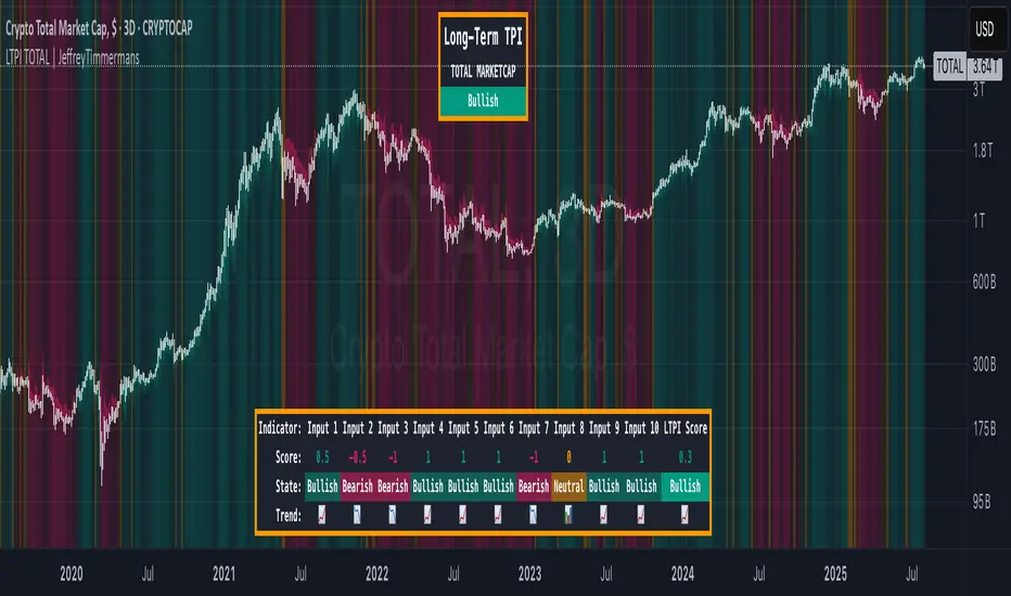
LTPI TOTAL | JeffreyTimmermansLong-Term Trend Probability Indicator
The "Long-Term Trend Probability Indicator" on TOTAL is a custom-built tool designed to analyze the global crypto market (TOTAL) from a long-term perspective. Unlike short-term indicators that react to price volatility, LTPI focuses on major trend shifts across the entire crypto market, helping to identify major trend shifts early.
This version of the LTPI is applied to the TOTAL market cap, making it a broad trend following tool.
Key Features
Long-Term Focus:
Designed for macro market analysis with less sensitivity to short-term noise.
10 Input Signals:
Combines 10 carefully selected inputs (trend following indicators) into a single score that reflects the overall market condition.
Market Regimes:
Classifies the TOTAL market into:
Bullish: Strong uptrend, expansion phase
Bearish: Strong downtrend, contraction phase
Neutral: Transitional or uncertain
Visual Background:
Background colors clearly display which regime is active.
Comprehensive Dashboard:
The panel at the bottom shows each input’s state, the composite LTPI score, and the resulting market trend.
How It Works
Inputs Analysis:
Each of the 10 inputs outputs one of three states:
+1 (Bullish)
-1 (Bearish)
0 (Neutral)
Score Calculation:
The total score is the sum of all 10 input signals divided by 10.
Score > 0.1 = Bullish
Score < -0.1 = Bearish
Between -0.1 and 0.1 = Neutral
Background Coloring:
Background colors dynamically adjust to reflect the long-term market regime.
Use Cases
Long-Term Positioning:
Identify periods of global expansion or contraction to position yourself accordingly.
Macro Confirmation:
Use LTPI in combination with medium-term (MTPI) and short-term tools for multi-timeframe confirmation.
Market Timing:
Alerts when LTPI crosses key thresholds help highlight the start of major bullish or bearish phases.
Dynamic Alerts:
Bullish Entry: LTPI score crosses above 0.1
Bearish Entry: LTPI score crosses below -0.1
Neutral Zone: Score moves back between -0.1 and 0.1
Conclusion
The Long-Term Trend Probability Indicator (LTPI – TOTAL) is a powerful tool for identifying long-term market phases across the entire crypto ecosystem. By focusing on long term trends and combining 10 inputs into a single probability score, it provides a clear macro perspective for strategic decision-making.
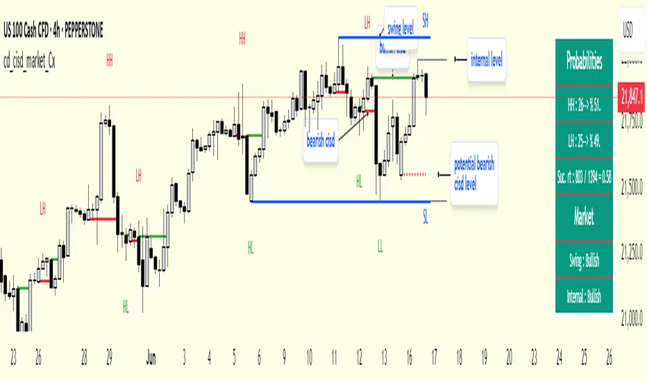
cd_cisd_market_CxHi Traders,
Overview:
Many traders follow market structure to identify the market direction and seek trade opportunities in line with the trend.
However, markings derived from user-defined inputs can create different structures, depending on personal choices. For instance, choosing a pivot distance of 3 instead of 2 alters the structure, even though the chart remains the same. Ideally, the structure should remain consistent.
"Change in State Delivery" ( CISD ) is a widely accepted concept among traders and is considered a significant indicator of market direction based on the gain/loss of CISD levels.
In this indicator, CISD is selected as the primary criterion for marking market structure, eliminating the influence of user-dependent variations.
Here is a summary of the key logic and rules applied:
• When the price forms a new high/low, that level is only considered a pivot if a CISD has occurred.
• A bullish CISD is always followed by a bearish CISD, and vice versa.
• Pivot points form the internal structure.
• The internal structure is used to interpret the swing structure.
• Probabilities are derived from internal structure patterns.
________________________________________
Details:
How is CISD determined?
As is commonly known:
• When price makes a new high, the opening level of the first candle in the consecutive bullish candle sequence is marked.
• When price makes a new low, the opening of the first candle in the consecutive bearish sequence is marked.
• If there’s only one candle in the sequence, its opening level is used.
In a bullish market, losing a bearish CISD level (i.e., a close below it) or in a bearish market, gaining a bullish CISD level (i.e., a close above it) is interpreted as a potential shift in buyer-seller dominance and a possible market reversal.
________________________________________
How are internal (pivot) levels determined?
• When price closes below a bearish CISD level, the highest candle's high becomes a pivot high (PH).
• When price closes above a bullish CISD level, the lowest candle's low becomes a pivot low (PL).
• If the new PH is above the previous PH, it’s labeled as HH (Higher High); otherwise, LH (Lower High).
• If the new PL is below the previous PL, it’s labeled as LL (Lower Low); otherwise, HL (Higher Low).
________________________________________
Internal Market Structure:
• A series of HHs indicates a bullish internal structure.
• A series of LLs indicates a bearish internal structure.
________________________________________
Swing (Main) Market Structure:
Using internal pivots and previous swing levels, the main market structure is derived.
• A new swing high (SH) requires the price to move above the previous SH.
• A new swing low (SL) requires the price to move below the previous SL.
________________________________________
Probability Calculation:
Pivot levels forming the internal structure are coded as five-element sequences.
There are 64 possible combinations of such sequences made from consecutive PH and PL values.
Each pattern’s frequency from its starting candle is tracked.
To make it more understandable:
For example, after the four-sequence “HH, LL, LH,HL”, either HH or LH might follow.
The table shows the statistical likelihood of both possible outcomes for the most recent four-element sequence on the chart.
________________________________________
How reliable is it?
To assess reliability, results are calculated from the beginning using:
Success Rate (Suc. Rt) = Number of Correct Predictions / Total Predictions
This value is added to the table for reference.
It’s important to note that no statistical outcome guarantees certainty—every result offers a different interpretation. What truly matters is to avoid getting stopped out 😊.
________________________________________
Menu Options:
Show/hide preferences and color selections can be customized via the indicator menu.
________________________________________
What’s Coming in Future Versions?
Features such as FVG (Fair Value Gaps) between swing levels, volume imbalances, order blocks / mitigation blocks, Fibonacci levels, and relevant trade suggestions will be added.
________________________________________
This is a BETA version that I believe will help simplify your market reading. I’d be happy to hear your feedback and suggestions.
Cheerful Trading!
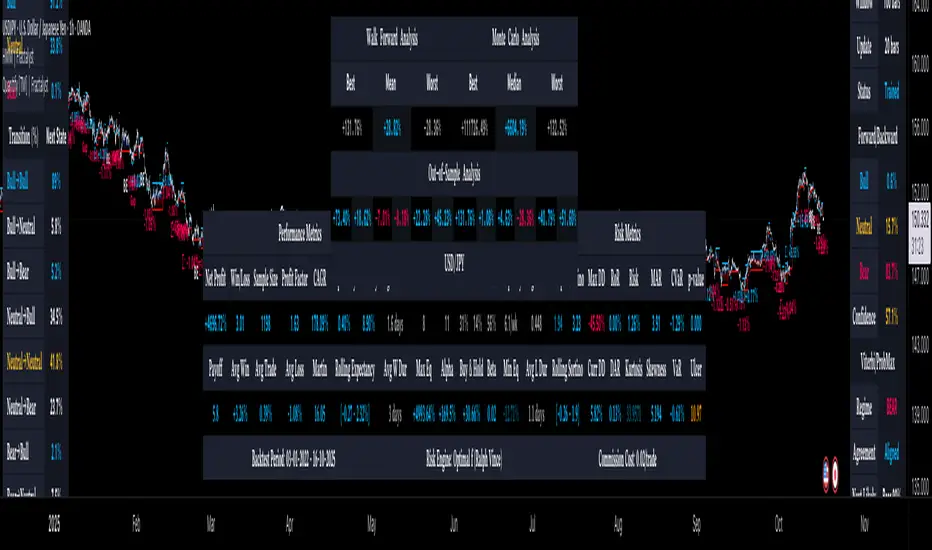
Quantify [Trading Model] | FractalystNote: In this description, "TM" refers to Trading Model (not trademark) and "EM" refers to Entry Model
What’s the indicator’s purpose and functionality?
You know how to identify market bias but always struggle with figuring out the best exit method, or even hesitating to take your trades?
I've been there. That's why I built this solution—once and for all—to help traders who know the market bias but need a systematic and quantitative approach for their entries and trade management.
A model that shows you real-time market probabilities and insights, so you can focus on execution with confidence—not doubt or FOMO.
How does this Quantify differentiate from Quantify ?
Have you managed to code or even found an indicator that identifies the market bias for you, so you don’t have to manually spend time analyzing the market and trend?
Then that’s exactly why you might need the Quantify Trading Model.
With the Trading Model (TM) version, the script automatically uses your given bias identification method to determine the trend (bull vs bear and neutral), detect the bias, and provide instant insight into the trades you could’ve taken.
To avoid complications from consecutive signals, it uses a kNN machine learning algorithm that processes market structure and probabilities to predict the best future patterns.
(You don’t have to deal with any complexity—it’s all taken care of for you.)
Quantify TM uses the k-Nearest Neighbors (kNN) machine learning algorithm to learn from historical market patterns and adapt to changing market structures. This means it can recognize similar market conditions from the past and apply those lessons to current trading decisions.
On the other hand, Quantify EM requires you to manually select your directional bias. It then focuses solely on generating entry signals based on that pre-determined bias.
While the entry model version (EM) uses your manual bias selection to determine the trend, it then provides insights into trades you could’ve taken and should be taking.
Trading Model (TM)
- Uses `input.source()` to incorporate your personal methodology for identifying market bias
- Automates everything—from bias detection to entry and exit decisions
- Adapts to market bias changes through kNN machine learning optimization
- Reduces human intervention in trading decisions, limiting emotional interference
Entry Model (EM)
- Focuses specifically on optimizing entry points within your pre-selected directional bias
- Requires manual input for determining market bias
- Provides entry signals without automating alerts or bias rules
Can the indicator be applied to any market approach/trading strategy?
Yes, if you have clear rules for identifying the market bias, then you can code your bias detection and then use the input.source() user input to retrieve the direction from your own indicator, then the Quantify uses machine-learning identify the best setups for you.
Here's an example:
//@version=6
indicator('Moving Averages Bias', overlay = true)
// Input lengths for moving averages
ma10_length = input.int(10, title = 'MA 10 Length')
ma20_length = input.int(20, title = 'MA 20 Length')
ma50_length = input.int(50, title = 'MA 50 Length')
// Calculate moving averages
ma10 = ta.sma(close, ma10_length)
ma20 = ta.sma(close, ma20_length)
ma50 = ta.sma(close, ma50_length)
// Identify bias
var bias = 0
if close > ma10 and close > ma20 and close > ma50 and ma10 > ma20 and ma20 > ma50
bias := 1 // Bullish
bias
else if close < ma10 and close < ma20 and close < ma50 and ma10 < ma20 and ma20 < ma50
bias := -1 // Bearish
bias
else
bias := 0 // Neutral
bias
// Plot the bias
plot(bias, title = 'Identified Bias', color = color.blue,display = display.none)
Once you've created your custom bias indicator, you can integrate it with Quantify :
- Add your bias indicator to your chart
- Open the Quantify settings
- Set the Bias option to "Auto"
- Select your custom indicator as the bias source
The machine learning algorithms will then analyze historical price action and identify optimal setups based on your defined bias parameters. Performance statistics are displayed in summary tables, allowing you to evaluate effectiveness across different timeframes.
Can the indicator be used for different timeframes or trading styles?
Yes, regardless of the timeframe you’d like to take your entries, the indicator adapts to your trading style.
Whether you’re a swing trader, scalper, or even a position trader, the algorithm dynamically evaluates market conditions across your chosen timeframe.
How Quantify Helps You Trade Profitably?
The Quantify Trading Model offers several powerful features that can significantly improve your trading profitability when used correctly:
Real-Time Edge Assessment
It displays real-time probability of price moving in your favor versus hitting your stoploss
This gives you immediate insight into risk/reward dynamics before entering trades
You can make more informed decisions by knowing the statistical likelihood of success
Historical Edge Validation
Instantly shows whether your trading approach has demonstrated an edge in historical data
Prevents you from trading setups that historically haven't performed well
Gives confidence when entering trades that have proven statistical advantages
Optimized Position Sizing
Analyzes each setup's success rate to determine the adjusted Kelly criterion formula
Customizes position sizing based on your selected maximum drawdown tolerance
Helps prevent account-destroying losses while maximizing growth potential
Advanced Exit Management
Utilizes market structure-based trailing stop-loss mechanisms
Maximizes the average risk-reward ratio profit per winning trade
Helps capture larger moves while protecting gains during market reversals
Emotional Discipline Enforcement
Eliminates emotional bias by adhering to your pre-defined rules for market direction
Prevents impulsive decisions by providing objective entry and exit signals
Creates psychological distance between your emotions and trading decisions
Overtrading Prevention
Highlights only setups that demonstrate positive expectancy
Reduces frequency of low-probability trades
Conserves capital for higher-quality opportunities
Systematic Approach Benefits
By combining machine learning algorithms with your personal bias identification methods, Quantify helps transform discretionary trading approaches into more systematic, probability-based strategies.
What Entry Models are used in Quantify Trading Model version?
The Quantify Trading Model utilizes two primary entry models to identify high-probability trade setups:
Breakout Entry Model
- Identifies potential trade entries when price breaks through significant swing highs and swing lows
- Captures momentum as price moves beyond established trading ranges
- Particularly effective in trending markets when combined with the appropriate bias detection
- Optimized by machine learning to filter false breakouts based on historical performance
Fractals Entry Model
- Utilizes fractal patterns to identify potential reversal or continuation points
- Also uses swing levels to determine optimal entry locations
- Based on the concept that market structure repeats across different timeframes
- Identifies local highs and lows that form natural entry points
- Enhanced by machine learning to recognize the most profitable fractal formations
- These entry models work in conjunction with your custom bias indicator to ensure trades are taken in the direction of the overall market trend. The machine learning component analyzes historical performance of these entry types across different market conditions to optimize entry timing and signal quality.
How Does This Indicator Identify Market Structure?
1. Swing Detection
• The indicator identifies key swing points on the chart. These are local highs or lows where the price reverses direction, forming the foundation of market structure.
2. Structural Break Validation
• A structural break is flagged when a candle closes above a previous swing high (bullish) or below a previous swing low (bearish).
• Break Confirmation Process:
To confirm the break, the indicator applies the following rules:
• Valid Swing Preceding the Break: There must be at least one valid swing point before the break.
3. Numeric Labeling
• Each confirmed structural break is assigned a unique numeric ID starting from 1.
• This helps traders track breaks sequentially and analyze how the market structure evolves over time.
4. Liquidity and Invalidation Zones
• For every confirmed structural break, the indicator highlights two critical zones:
1. Liquidity Zone (LIQ): Represents the structural liquidity level.
2. Invalidation Zone (INV): Acts as Invalidation point if the structure fails to hold.
How does the trailing stop-loss work? what are the underlying calculations?
A trailing stoploss is a dynamic risk management tool that moves with the price as the market trend continues in the trader’s favor. Unlike a fixed take profit, which stays at a set level, the trailing stoploss automatically adjusts itself as the market moves, locking in profits as the price advances.
In Quantify, the trailing stoploss is enhanced by incorporating market structure liquidity levels (explain above). This ensures that the stoploss adjusts intelligently based on key price levels, allowing the trader to stay in the trade as long as the trend remains intact, while also protecting profits if the market reverses.
What is the Kelly Criterion, and how does it work in Quantify?
The Kelly Criterion is a mathematical formula used to determine the optimal position size for each trade, maximizing long-term growth while minimizing the risk of large drawdowns. It calculates the percentage of your portfolio to risk on a trade based on the probability of winning and the expected payoff.
Quantify integrates this with user-defined inputs to dynamically calculate the most effective position size in percentage, aligning with the trader’s risk tolerance and desired exposure.
How does Quantify use the Kelly Criterion in practice?
Quantify uses the Kelly Criterion to optimize position sizing based on the following factors:
1. Confidence Level: The model assesses the confidence level in the trade setup based on historical data and sample size. A higher confidence level increases the suggested position size because the trade has a higher probability of success.
2. Max Allowed Drawdown (User-Defined): Traders can set their preferred maximum allowed drawdown, which dictates how much loss is acceptable before reducing position size or stopping trading. Quantify uses this input to ensure that risk exposure aligns with the trader’s risk tolerance.
3. Probabilities: Quantify calculates the probabilities of success for each trade setup. The higher the probability of a successful trade (based on historical price action and liquidity levels), the larger the position size suggested by the Kelly Criterion.
How can I get started to use the indicator?
1. Set Your Market Bias
• Choose Auto.
• Select the source you want Quantify to use as for bias identification method (explained above)
2. Choose Your Entry Timeframes
• Specify the timeframes you want to focus on for trade entries.
• The indicator will dynamically analyze these timeframes to provide optimal setups.
3. Choose Your Entry Model and BE/TP Levels
• Choose a model that suits your personality
• Choose a level where you'd like the script to take profit or move stop-loss to BE
4. Set and activate the alerts
What tables are used in the Quantify?
• Quarterly
• Monthly
• Weekly
Terms and Conditions | Disclaimer
Our charting tools are provided for informational and educational purposes only and should not be construed as financial, investment, or trading advice. They are not intended to forecast market movements or offer specific recommendations. Users should understand that past performance does not guarantee future results and should not base financial decisions solely on historical data.
Built-in components, features, and functionalities of our charting tools are the intellectual property of @Fractalyst Unauthorized use, reproduction, or distribution of these proprietary elements is prohibited.
- By continuing to use our charting tools, the user acknowledges and accepts the Terms and Conditions outlined in this legal disclaimer and agrees to respect our intellectual property rights and comply with all applicable laws and regulations.
QuantBuilder | FractalystWhat's the strategy's purpose and functionality?
QuantBuilder is designed for both traders and investors who want to utilize mathematical techniques to develop profitable strategies through backtesting on historical data.
The primary goal is to develop profitable quantitive strategies that not only outperform the underlying asset in terms of returns but also minimize drawdown.
For instance, consider Bitcoin (BTC), which has experienced significant volatility, averaging an estimated 200% annual return over the past decade, with maximum drawdowns exceeding -80%. By employing this strategy with diverse entry and exit techniques, users can potentially seek to enhance their Compound Annual Growth Rate (CAGR) while managing risk to maintain a lower maximum drawdown.
While this strategy employs quantitative techniques, including mathematical methods such as probabilities and positive expected values, it demonstrates exceptional efficacy across all markets. It particularly excels in futures, indices, stocks, cryptocurrencies, and commodities, leveraging their inherent trending behaviors for optimized performance.
In both trending and consolidating market conditions, QuantBuilder employs a combination of multi-timeframe probabilities, expected values, directional biases, moving averages and diverse entry models to identify and capitalize on bullish market movements.
How does the strategy perform for both investors and traders?
The strategy has two main modes, tailored for different market participants: Traders and Investors.
1. Trading:
- Designed for traders looking to capitalize on bullish markets.
- Utilizes a percentage risk per trade to manage risk and optimize returns.
- Suitable for both swing and intraday trading with a focus on probabilities and risk per trade approach.
2. Investing:
- Geared towards investors who aim to capitalize on bullish trending markets without using leverage while mitigating the asset's maximum drawdown.
- Utilizes pre-define percentage of the equity to buy, hold, and manage the asset.
- Focuses on long-term growth and capital appreciation by fully/partially investing in the asset during bullish conditions.
How does the strategy identify market structure? What are the underlying calculations?
The strategy utilizes an efficient logic with for loops to pinpoint the first swing candle featuring a pivot of 2, establishing the point at which the break of structure begins.
What entry criteria are used in this script? What are the underlying calculations?
The script utilizes two entry models: BreakOut and fractal.
Underlying Calculations:
Breakout: The script assigns the most recent swing high to a variable. When the price closes above this level and all other conditions are met, the script executes a breakout entry (conservative approach).
Fractal: The script identifies a swing low with a period of 2. Once this condition is met, the script executes the trade (aggressive approach).
How does the script calculate probabilities? What are the underlying calculations?
The script calculates probabilities by monitoring price interactions with liquidity levels. Here’s how the underlying calculations work:
Tracking Price Hits: The script counts the number of times the price taps into each liquidity side after the EQM level is activated. This data is stored in an array for further analysis.
Sample Size Consideration: The total number of price interactions serves as the sample size for calculating probabilities.
Probability Calculation: For each liquidity side, the script calculates the probability by taking the average of the recorded hits. This allows for a dynamic assessment of the likelihood that a particular side will be hit next, based on historical performance.
Dynamic Adjustment: As new price data comes in, the probabilities are recalculated, providing real-time aduptive insights into market behavior.
Note: The calculations are performed independently for each directional range. A range is considered bearish if the previous breakout was through a sellside liquidity. Conversely, a range is considered bullish if the most recent breakout was through a buyside liquidity.
How does the script calculate expected values? What are the underlying calculations?
The script calculates expected values by leveraging the probabilities of winning and losing trades, along with their respective returns. The process involves the following steps:
This quantitative methodology provides a robust framework for assessing the expected performance of trading strategies based on historical data and backtesting results.
How is the contextual bias calculated? What are the underlying calculations?
The contextual bias in the QuantBuilder script is calculated through a structured approach that assesses market structure based on swing highs and lows. Here’s how it works:
Identification of Swing Points: The script identifies significant swing points using a defined pivot logic, focusing on the first swing high and swing low. This helps establish critical levels for determining market structure.
Break of Structure (BOS) Assessment:
Bullish BOS: The script recognizes a bullish break of structure when a candle closes above the first swing high, followed by at least one swing low.
Bearish BOS: Conversely, a bearish break of structure is identified when a candle closes below the first swing low, followed by at least one swing high.
Bias Assignment: Based on the identified break of structure, the script assigns directional biases:
A bullish bias is assigned if a bullish BOS is confirmed.
A bearish bias is assigned if a bearish BOS is confirmed.
Quantitative Evaluation: Each identified bias is quantitatively evaluated, allowing the script to assign numerical values representing the strength of each bias. This quantification aids in assessing the reliability of market sentiment across multiple timeframes.
What's the purpose of using moving averages in this strategy? What are the underlying calculations?
Using moving averages is a widely-used technique to trade with the trend.
The main purpose of using moving averages in this strategy is to filter out bearish price action and to only take trades when the price is trading ABOVE specified moving averages.
The script uses different types of moving averages with user-adjustable timeframes and periods/lengths, allowing traders to try out different variations to maximize strategy performance and minimize drawdowns.
By applying these calculations, the strategy effectively identifies bullish trends and avoids market conditions that are not conducive to profitable trades.
The MA filter allows traders to choose whether they want a specific moving average above or below another one as their entry condition.
What type of stop-loss identification method are used in this strategy? What are the underlying calculations?
- Initial Stop-loss:
1. ATR Based:
The Average True Range (ATR) is a method used in technical analysis to measure volatility. It is not used to indicate the direction of price but to measure volatility, especially volatility caused by price gaps or limit moves.
Calculation:
- To calculate the ATR, the True Range (TR) first needs to be identified. The TR takes into account the most current period high/low range as well as the previous period close.
The True Range is the largest of the following:
- Current Period High minus Current Period Low
- Absolute Value of Current Period High minus Previous Period Close
- Absolute Value of Current Period Low minus Previous Period Close
- The ATR is then calculated as the moving average of the TR over a specified period. (The default period is 14)
2. ADR Based:
The Average Day Range (ADR) is an indicator that measures the volatility of an asset by showing the average movement of the price between the high and the low over the last several days.
Calculation:
- To calculate the ADR for a particular day:
- Calculate the average of the high prices over a specified number of days.
- Calculate the average of the low prices over the same number of days.
- Find the difference between these average values.
- The default period for calculating the ADR is 14 days. A shorter period may introduce more noise, while a longer period may be slower to react to new market movements.
3. PL Based:
This method places the stop-loss at the low of the previous candle.
If the current entry is based on the hunt entry strategy, the stop-loss will be placed at the low of the candle that wicks through the lower FRMA band.
Example:
If the previous candle's low is 100, then the stop-loss will be set at 100.
This method ensures the stop-loss is placed just below the most recent significant low, providing a logical and immediate level for risk management.
- Trailing Stop-Loss:
One of the key elements of this strategy is its ability to detect structural liquidity and structural invalidation levels across multiple timeframes to trail the stop-loss once the trade is in running profits.
By utilizing this approach, the strategy allows enough room for price to run.
By using these methods, the strategy dynamically adjusts the initial stop-loss based on market volatility, helping to protect against adverse price movements while allowing for enough room for trades to develop.
Each market behaves differently across various timeframes, and it is essential to test different parameters and optimizations to find out which trailing stop-loss method gives you the desired results and performance.
What type of break-even and take profit identification methods are used in this strategy? What are the underlying calculations?
For Break-Even:
Percentage (%) Based:
Moves the initial stop-loss to the entry price when the price reaches a certain percentage above the entry.
Calculation:
Break-even level = Entry Price * (1 + Percentage / 100)
Example:
If the entry price is $100 and the break-even percentage is 5%, the break-even level is $100 * 1.05 = $105.
Risk-to-Reward (RR) Based:
Moves the initial stop-loss to the entry price when the price reaches a certain RR ratio.
Calculation:
Break-even level = Entry Price + (Initial Risk * RR Ratio)
For TP1 (Take Profit 1):
- You can choose to set a take profit level at which your position gets fully closed or 50% if the TP2 boolean is enabled.
- Similar to break-even, you can select either a percentage (%) or risk-to-reward (RR) based take profit level, allowing you to set your TP1 level as a percentage amount above the entry price or based on RR.
For TP2 (Take Profit 2):
- You can choose to set a take profit level at which your position gets fully closed.
- As with break-even and TP1, you can select either a percentage (%) or risk-to-reward (RR) based take profit level, allowing you to set your TP2 level as a percentage amount above the entry price or based on RR.
What's the day filter Filter, what does it do?
The day filter allows users to customize the session time and choose the specific days they want to include in the strategy session. This helps traders tailor their strategies to particular trading sessions or days of the week when they believe the market conditions are more favorable for their trading style.
Customize Session Time:
Users can define the start and end times for the trading session.
This allows the strategy to only consider trades within the specified time window, focusing on periods of higher market activity or preferred trading hours.
Select Days:
Users can select which days of the week to include in the strategy.
This feature is useful for excluding days with historically lower volatility or unfavorable trading conditions (e.g., Mondays or Fridays).
Benefits:
Focus on Optimal Trading Periods:
By customizing session times and days, traders can focus on periods when the market is more likely to present profitable opportunities.
Avoid Unfavorable Conditions:
Excluding specific days or times can help avoid trading during periods of low liquidity or high unpredictability, such as major news events or holidays.
What tables are available in this script?
- Summary: Provides a general overview, displaying key performance parameters such as Net Profit, Profit Factor, Max Drawdown, Average Trade, Closed Trades and more.
Total Commission: Displays the cumulative commissions incurred from all trades executed within the selected backtesting window. This value is derived by summing the commission fees for each trade on your chart.
Average Commission: Represents the average commission per trade, calculated by dividing the Total Commission by the total number of closed trades. This metric is crucial for assessing the impact of trading costs on overall profitability.
Avg Trade: The sum of money gained or lost by the average trade generated by a strategy. Calculated by dividing the Net Profit by the overall number of closed trades. An important value since it must be large enough to cover the commission and slippage costs of trading the strategy and still bring a profit.
MaxDD: Displays the largest drawdown of losses, i.e., the maximum possible loss that the strategy could have incurred among all of the trades it has made. This value is calculated separately for every bar that the strategy spends with an open position.
Profit Factor: The amount of money a trading strategy made for every unit of money it lost (in the selected currency). This value is calculated by dividing gross profits by gross losses.
Avg RR: This is calculated by dividing the average winning trade by the average losing trade. This field is not a very meaningful value by itself because it does not take into account the ratio of the number of winning vs losing trades, and strategies can have different approaches to profitability. A strategy may trade at every possibility in order to capture many small profits, yet have an average losing trade greater than the average winning trade. The higher this value is, the better, but it should be considered together with the percentage of winning trades and the net profit.
Winrate: The percentage of winning trades generated by a strategy. Calculated by dividing the number of winning trades by the total number of closed trades generated by a strategy. Percent profitable is not a very reliable measure by itself. A strategy could have many small winning trades, making the percent profitable high with a small average winning trade, or a few big winning trades accounting for a low percent profitable and a big average winning trade. Most mean-reversion successful strategies have a percent profitability of 40-80% but are profitable due to risk management control.
BE Trades: Number of break-even trades, excluding commission/slippage.
Losing Trades: The total number of losing trades generated by the strategy.
Winning Trades: The total number of winning trades generated by the strategy.
Total Trades: Total number of taken traders visible your charts.
Net Profit: The overall profit or loss (in the selected currency) achieved by the trading strategy in the test period. The value is the sum of all values from the Profit column (on the List of Trades tab), taking into account the sign.
- Monthly: Displays performance data on a month-by-month basis, allowing users to analyze performance trends over each month and year.
- Weekly: Displays performance data on a week-by-week basis, helping users to understand weekly performance variations.
- UI Table: A user-friendly table that allows users to view and save the selected strategy parameters from user inputs. This table enables easy access to key settings and configurations, providing a straightforward solution for saving strategy parameters by simply taking a screenshot with Alt + S or ⌥ + S.
User-input styles and customizations:
To facilitate studying historical data, all conditions and filters can be applied to your charts. By plotting background colors on your charts, you'll be able to identify what worked and what didn't in certain market conditions.
Please note that all background colors in the style are disabled by default to enhance visualization.
How to Use This Quantitive Strategy Builder to Create a Profitable Edge and System?
Choose Your Strategy mode:
- Decide whether you are creating an investing strategy or a trading strategy.
Select a Market:
- Choose a one-sided market such as stocks, indices, or cryptocurrencies.
Historical Data:
- Ensure the historical data covers at least 10 years of price action for robust backtesting.
Timeframe Selection:
- Choose the timeframe you are comfortable trading with. It is strongly recommended to use a timeframe above 15 minutes to minimize the impact of commissions/slippage on your profits.
Set Commission and Slippage:
- Properly set the commission and slippage in the strategy properties according to your broker/prop firm specifications.
Parameter Optimization:
- Use trial and error to test different parameters until you find the performance results you are looking for in the summary table or, preferably, through deep backtesting using the strategy tester.
Trade Count:
- Ensure the number of trades is 200 or more; the higher, the better for statistical significance.
Positive Average Trade:
- Make sure the average trade is above zero.
(An important value since it must be large enough to cover the commission and slippage costs of trading the strategy and still bring a profit.)
Performance Metrics:
- Look for a high profit factor, and net profit with minimum drawdown.
- Ideally, aim for a drawdown under 20-30%, depending on your risk tolerance.
Refinement and Optimization:
- Try out different markets and timeframes.
- Continue working on refining your edge using the available filters and components to further optimize your strategy.
What makes this strategy original?
QuantBuilder stands out due to its unique combination of quantitative techniques and innovative algorithms that leverage historical data for real-time trading decisions. Unlike most algorithmic strategies that work based on predefined rules, this strategy adapts to real-time market probabilities and expected values, enhancing its reliability. Key features include:
Mathematical Framework: The strategy integrates advanced mathematical concepts, such as probabilities and expected values, to assess trade viability and optimize decision-making.
Multi-Timeframe Analysis: By utilizing multi-timeframe probabilities, QuantBuilder provides a comprehensive view of market conditions, enhancing the accuracy of entry and exit points.
Dynamic Market Structure Identification: The script employs a systematic approach to identify market structure changes, utilizing a blend of swing highs and lows to detect contextual/direction bias of the market.
Built-in Trailing Stop Loss: The strategy features a dynamic trailing stop loss based on multi-timeframe analysis of market structure. This allows traders to lock in profits while adapting to changing market conditions, ensuring that exits are executed at optimal levels without prematurely closing positions.
Robust Performance Metrics: With detailed performance tables and visualizations, users can easily evaluate strategy effectiveness and adjust parameters based on historical performance.
Adaptability: The strategy is designed to work across various markets and timeframes, making it versatile for different trading styles and objectives.
Suitability for Investors and Traders: QuantBuilder is ideal for both investors and traders looking to rely on mathematically proven data to create profitable strategies, ensuring that decisions are grounded in quantitative analysis.
These original elements combine to create a powerful tool that can help both traders and investors to build and refine profitable strategies based on algorithmic quantitative analysis.
Terms and Conditions | Disclaimer
Our charting tools are provided for informational and educational purposes only and should not be construed as financial, investment, or trading advice. They are not intended to forecast market movements or offer specific recommendations. Users should understand that past performance does not guarantee future results and should not base financial decisions solely on historical data.
Built-in components, features, and functionalities of our charting tools are the intellectual property of @Fractalyst Unauthorized use, reproduction, or distribution of these proprietary elements is prohibited.
By continuing to use our charting tools, the user acknowledges and accepts the Terms and Conditions outlined in this legal disclaimer and agrees to respect our intellectual property rights and comply with all applicable laws and regulations.

OrderFlow [Adjustable] | FractalystWhat's the indicator's purpose and functionality?
This indicator is designed to assist traders in identifying real-time probabilities of buyside and sellside liquidity .
It allows for an adjustable pivot level , enabling traders to customize the level they want to use for their entries.
By doing so, traders can evaluate whether their chosen entry point would yield a positive expected value over a large sample size, optimizing their strategy for long-term profitability.
For advanced traders looking to enhance their analysis, the indicator supports the incorporation of up to 7 higher timeframe biases .
Additionally, the higher timeframe pivot level can be adjusted according to the trader's preferences,
Offering maximum adaptability to different strategies and needs, further helping to maximize positive EV.
EV=(P(Win)×R(Win))−(P(Loss)×R(Loss))
-----
What's the purpose of these levels? What are the underlying calculations?
1. Understanding Swing highs and Swing Lows
Swing High: A Swing High is formed when there is a high with 2 lower highs to the left and right.
Swing Low: A Swing Low is formed when there is a low with 2 higher lows to the left and right.
2. Understanding the purpose and the underlying calculations behind Buyside, Sellside and Pivot levels.
3. Identifying Discount and Premium Zones.
4. Importance of Risk-Reward in Premium and Discount Ranges
----
How does the script calculate probabilities?
The script calculates the probability of each liquidity level individually. Here's the breakdown:
1. Upon the formation of a new range, the script waits for the price to reach and tap into pivot level level. Status: "⏸" - Inactive
2. Once pivot level is tapped into, the pivot status becomes activated and it waits for either liquidity side to be hit. Status: "▶" - Active
3. If the buyside liquidity is hit, the script adds to the count of successful buyside liquidity occurrences. Similarly, if the sellside is tapped, it records successful sellside liquidity occurrences.
4. Finally, the number of successful occurrences for each side is divided by the overall count individually to calculate the range probabilities.
Note: The calculations are performed independently for each directional range. A range is considered bearish if the previous breakout was through a sellside liquidity. Conversely, a range is considered bullish if the most recent breakout was through a buyside liquidity.
----
What does the multi-timeframe functionality offer?
In the adjustable version of the orderflow indicator, you can incorporate up to 7 higher timeframe probabilities directly into the table.
This feature allows you to analyze the probabilities of buyside and sellside liquidity across multiple timeframes, without the need to manually switch between them.
By viewing these higher timeframe probabilities in one place, traders can spot larger market trends and refine their entries and exits with a better understanding of the overall market context.
This multi-timeframe functionality helps traders:
1. Simplify decision-making by offering a comprehensive view of multiple timeframes at once.
2. Identify confluence between timeframes, enhancing the confidence in trade setups.
3. Adapt strategies more effectively, as the higher timeframe pivot levels can be customized to meet individual preferences and goals.
----
What are the multi-timeframe underlying calculations?
The script uses the same calculations (mentioned above) and uses security function to request the data such as price levels, bar time, probabilities and booleans from the user-input timeframe.
----
How does the Indicator Identifies Positive Expected Values?
OrderFlow indicator instantly calculates whether a trade setup has the potential for positive expected value (EV) in the long run.
To determine a positive EV setup, the indicator uses the formula:
EV=(P(Win)×R(Win))−(P(Loss)×R(Loss))
where:
P(Win) is the probability of a winning trade.
R(Win) is the reward or return for a winning trade, determined by the current risk-to-reward ratio (RR).
P(Loss) is the probability of a losing trade.
R(Loss) is the loss incurred per losing trade, typically assumed to be -1.
By calculating these values based on historical data and the current trading setup, the indicator helps you understand whether your trade has a positive expected value over a large sample size.
----
How can I know that the setup I'm going to trade with has a postive EV?
If the indicator detects that the adjusted pivot and buy/sell side probabilities have generated positive expected value (EV) in historical data, the risk-to-reward (RR) label within the range box will be colored blue and red .
If the setup does not produce positive EV, the RR label will appear gray.
This indicates that even the risk-to-reward ratio is greater than 1:1, the setup is not likely to yield a positive EV because, according to historical data, the number of losses outweighs the number of wins relative to the RR gain per winning trade.
----
What is the confidence level in the indicator, and how is it determined?
The confidence level in the indicator reflects the reliability of the probabilities calculated based on historical data. It is determined by the sample size of the probabilities used in the calculations. A larger sample size generally increases the confidence level, indicating that the probabilities are more reliable and consistent with past performance.
----
How does the confidence level affect the risk-to-reward (RR) label?
The confidence level (★) is visually represented alongside the probability label. A higher confidence level indicates that the probabilities used to determine the RR label are based on a larger and more reliable sample size.
----
How can traders use the confidence level to make better trading decisions?
Traders can use the confidence level to gauge the reliability of the probabilities and expected value (EV) calculations provided by the indicator. A confidence level above 95% is considered statistically significant and indicates that the historical data supporting the probabilities is robust. This high confidence level suggests that the probabilities are reliable and that the indicator’s recommendations are more likely to be accurate.
In data science and statistics, a confidence level above 95% generally means that there is less than a 5% chance that the observed results are due to random variation. This threshold is widely accepted in research and industry as a marker of statistical significance. Studies such as those published in the Journal of Statistical Software and the American Statistical Association support this threshold, emphasizing that a confidence level above 95% provides a strong assurance of data reliability and validity.
Conversely, a confidence level below 95% indicates that the sample size may be insufficient and that the data might be less reliable . In such cases, traders should approach the indicator’s recommendations with caution and consider additional factors or further analysis before making trading decisions.
----
How does the sample size affect the confidence level, and how does it relate to my TradingView plan?
The sample size for calculating the confidence level is directly influenced by the amount of historical data available on your charts. A larger sample size typically leads to more reliable probabilities and higher confidence levels.
Here’s how the TradingView plans affect your data access:
Essential Plan
The Essential Plan provides basic data access with a limited amount of historical data. This can lead to smaller sample sizes and lower confidence levels, which may weaken the robustness of your probability calculations. Suitable for casual traders who do not require extensive historical analysis.
Plus Plan
The Plus Plan offers more historical data than the Essential Plan, allowing for larger sample sizes and more accurate confidence levels. This enhancement improves the reliability of indicator calculations. This plan is ideal for more active traders looking to refine their strategies with better data.
Premium Plan
The Premium Plan grants access to extensive historical data, enabling the largest sample sizes and the highest confidence levels. This plan provides the most reliable data for accurate calculations, with up to 20,000 historical bars available for analysis. It is designed for serious traders who need comprehensive data for in-depth market analysis.
PRO+ Plans
The PRO+ Plans offer the most extensive historical data, allowing for the largest sample sizes and the highest confidence levels. These plans are tailored for professional traders who require advanced features and significant historical data to support their trading strategies effectively.
For many traders, the Premium Plan offers a good balance of affordability and sufficient sample size for accurate confidence levels.
----
What is the HTF probability table and how does it work?
The HTF (Higher Time Frame) probability table is a feature that allows you to view buy and sellside probabilities and their status from timeframes higher than your current chart timeframe.
Here’s how it works:
Data Request : The table requests and retrieves data from user-defined higher timeframes (HTFs) that you select.
Probability Display: It displays the buy and sellside probabilities for each of these HTFs, providing insights into the likelihood of price movements based on higher timeframe data.
Detailed Tooltips: The table includes detailed tooltips for each timeframe, offering additional context and explanations to help you understand the data better.
----
What do the different colors in the HTF probability table indicate?
The colors in the HTF probability table provide visual cues about the expected value (EV) of trading setups based on higher timeframe probabilities:
Blue: Suggests that entering a long position from the HTF user-defined pivot point, targeting buyside liquidity, is likely to result in a positive expected value (EV) based on historical data and sample size.
Red: Indicates that entering a short position from the HTF user-defined pivot point, targeting sellside liquidity, is likely to result in a positive expected value (EV) based on historical data and sample size.
Gray: Shows that neither long nor short trades from the HTF user-defined pivot point are expected to generate positive EV, suggesting that trading these setups may not be favorable.
----
How to use the indicator effectively?
For Amateur Traders:
Start Simple: Begin by focusing on one timeframe at a time with the pivot level set to the default (50%). This helps you understand the basic functionality of the indicator.
Entry and Exit Strategy: Focus on entering trades at the pivot level while targeting the higher probability side for take profit and the lower probability side for stop loss.
Use simulation or paper trading to practice this strategy.
Adjustments: Once you have a solid understanding of how the indicator works, you can start adjusting the pivot level to other values that suit your strategy.
Ensure that the RR labels are colored (blue or red) to indicate positive EV setups before executing trades.
For Advanced Traders:
1. Select Higher Timeframe Bias: Choose a higher timeframe (HTF) as your main bias. Start with the default pivot level and ensure the confidence level is above 95% to validate the probabilities.
2. Align Lower Timeframes: Switch between lower timeframes to identify which ones align with your predefined HTF bias. This helps in synchronizing your trading decisions across different timeframes.
3. Set Entries with Current Pivot Level: Use the current pivot level for trade entries. Ensure the HTF status label is active, indicating that the probabilities are valid and in play.
4. Target HTF Liquidity Level: Aim for liquidity levels that correspond to the higher timeframe, as these levels are likely to offer better trading opportunities.
5. Adjust Pivot Levels: As you gain experience, adjust the pivot levels to further optimize your strategy for high EV. Fine-tune these levels based on the aggregated data from multiple timeframes.
6. Practice on Paper Trading: Test your strategies through paper trading to eliminate discretion and refine your approach without financial risk.
7. Focus on Trade Management: Ultimately, effective trade management is crucial. Concentrate on managing your trades well to ensure long-term success. By aiming for setups that produce positive EV, you can position yourself similarly to how a casino operates.
----
🎲 Becoming the House (Gaining Edge Over the Market):
In American roulette, the house has a 5.26% edge due to the 0 and 00. This means that while players have a 47.37% chance of winning on even-money bets, the true odds are 50%. The discrepancy between the true odds and the payout ensures that, statistically, the casino will win over time.
From the Trader's Perspective: In trading, you gain an edge by focusing on setups with positive expected value (EV). If you have a 55.48% chance of winning with a 1:1 risk-to-reward ratio, your setup has a higher probability of profitability than the losing side. By consistently targeting such setups and managing your trades effectively, you create a statistical advantage, similar to the casino’s edge.
----
🎰 Applying the Concept to Trading:
Just as casinos rely on their mathematical edge, you can achieve long-term success in trading by focusing on setups with positive EV. By ensuring that your probabilities and risk-to-reward (RR) ratios are in your favor, you create an edge similar to that of the house.
And by systematically targeting trades with favorable probabilities and managing your trades effectively, you improve your chances of profitability over the long run. Which is going to help you “become the house” in your trading, leveraging statistical advantages to enhance your overall performance.
----
What makes this indicator original?
Real-Time Probability Calculations: The indicator provides real-time calculations of buy and sell probabilities based on historical data, allowing traders to assess the likelihood of positive expected value (EV) setups instantly.
Adjustable Pivot Levels: It features an adjustable pivot level that traders can modify according to their preferences, enhancing the flexibility to align with different trading strategies.
Multi-Timeframe Integration: The indicator supports up to 7 higher timeframes, displaying their probabilities and biases in a single view, which helps traders make informed decisions without switching timeframes.
Confidence Levels: It includes confidence levels based on sample sizes, offering insights into the reliability of the probabilities. Traders can gauge the strength of the data before making trades.
Dynamic EV Labels: The indicator provides color-coded EV labels that change based on the validity of the setup. Blue indicates positive EV in a long bias, red indicates positive EV in a short bias and gray signals caution, making it easier for traders to identify high-quality setups.
HTF Probability Table: The HTF probability table displays buy and sell probabilities from user-defined higher timeframes, helping traders integrate broader market context into their decision-making process.
----
Terms and Conditions | Disclaimer
Our charting tools are provided for informational and educational purposes only and should not be construed as financial, investment, or trading advice. They are not intended to forecast market movements or offer specific recommendations. Users should understand that past performance does not guarantee future results and should not base financial decisions solely on historical data.
Built-in components, features, and functionalities of our charting tools are the intellectual property of @Fractalyst use, reproduction, or distribution of these proprietary elements is prohibited.
By continuing to use our charting tools, the user acknowledges and accepts the Terms and Conditions outlined in this legal disclaimer and agrees to respect our intellectual property rights and comply with all applicable laws and regulations.

Price Close ProbabilityThe Price Close Probability Indicator is designed to help traders estimate the likelihood of price closing above or below specified levels within a given bar. By placing two levels on your chart, you can quickly gauge the probability of the current price bar closing above or below these levels in real-time.
Key Features:
Dynamic Probability Calculation: The indicator continuously updates the probability of price closing above or below your set levels as the current bar progresses, providing you with timely insights as the bar approaches its close.
Customizable Standard Deviation : Adjust the length of the Standard Deviation used in the calculations to tailor the probability estimates to your preferred settings.
User-Friendly Probability Table : A clean, easy-to-read table displays the calculated probabilities, helping you make informed trading decisions at a glance.
Assumptions and Considerations:
While the indicator assumes that returns are normally distributed, which may not fully reflect reality, it still offers a valuable approximation of the probabilities for price movement within the current bar.
Future Enhancements (Coming Soon):
Multi-Bar Probability: Calculate probabilities across multiple bars to enhance your forecasting capabilities.
Additional Levels: Set more than two levels for a broader analysis of price movements.
Refined Distribution Modeling: Improve the accuracy of probability calculations by adjusting for more realistic return distributions.
Disclaimer
Please remember that past performance may not be indicative of future results.
Due to various factors, including changing market conditions, the strategy may no longer perform as well as in historical backtesting.
This post and the script don’t provide any financial advice.

OrderFlow [Probabilities] | FractalystWhat's the indicator's purpose and functionality?
The indicator is designed to incorporate probabilities with buyside and sellside liquidity, as well as premium and discount ranges within the market. It also provides traders with a multi-timeframe functionality for observing liquidity levels and probabilities across two timeframes without the need to manually switch between them.
These levels are often used in smart money trading concepts for identifying key areas of interest, such as potential reversal points, areas of accumulation or distribution, and zones of high liquidity.
----
What's the purpose of these levels? What are the underlying calculations?
1. Understanding Swing highs and Swing Lows
Swing High: A Swing High is formed when there is a high with 2 lower highs to the left and right.
Swing Low: A Swing Low is formed when there is a low with 2 higher lows to the left and right.
2. Understanding the purpose and the underlying calculations behind Buyside , Sellside and Equilibrium levels.
3. Identifying Discount and Premium Zones.
4. Importance of Risk-Reward in Premium and Discount Ranges
----
How does the script calculate probabilities?
The script calculates the probability of each liquidity level individually. Here's the breakdown:
1. Upon the formation of a new range, the script waits for the price to reach and tap into equilibrium or the 50% level. Status: "⏸" - Inactive
2. Once equilibrium is tapped into, the equilibrium status becomes activated and it waits for either liquidity side to be hit. Status: "▶" - Active
3. If the buyside liquidity is hit, the script adds to the count of successful buyside liquidity occurrences. Similarly, if the sellside is tapped, it records successful sellside liquidity occurrences.
5. Finally, the number of successful occurrences for each side is divided by the overall count individually to calculate the range probabilities.
Note: The calculations are performed independently for each directional range. A range is considered bearish if the previous breakout was through a sellside liquidity. Conversely, a range is considered bullish if the most recent breakout was through a buyside liquidity.
----
What does the multi-timeframe functionality offer?
Enabling and selecting a higher timeframe in the indicator's user-input settings allows you to access not only the current range information but also the liquidity sides, status, price levels, and probabilities of a higher timeframe without needing to switch between timeframes and mark up the levels manually.
----
What are the multi-timeframe underlying calculations?
The script uses the same calculations (mentioned above) and requests the data such as price levels, bar time, probabilities and booleans from the user-input timeframe.
Non-repainting Security Function with Lookahead ON
//Function to fetch data for a given timeframe
getHTFData(timeframe_,exp_) =>
request.security(syminfo.tickerid, timeframe_,exp_ ,lookahead = barmerge.lookahead_on)
----
How to use the indicator?
1. Add the indicator to your TradingView chart.
2. Choose the pair you want to analyze/trade.
3. Enable the HTF in user-input settings and choose a timeframe as for your higher timeframe bias.
4. (Important) : Ensure that the probabilities on both timeframes are aligned in one direction. If not, switch between timeframes until you find a pair of timeframes that are in line with each other and have higher probabilities on one liquidity side.
For Swing traders:
Use Hourly timeframes (1H/2H/4H/8H/12H) as your current timeframe and 1D/3D/1W/2W for your higher timeframe (HTF).
Entry: Hourly Equilibrium level. (Limit order)
Stoploss: Place it on the side where the probability is lower than 50%.
Break-even level/TP1: Hourly breakout of the liquidity.
TP2: Target the Higher Timeframe (HTF) liquidity level where the probability is higher than 50%.
2H/1D COINBASE:BTCUSD
For Day traders:
Use minutely timeframes (5m/15m/30m) as your current timeframe and 1H/2H/4H/8H/12H for your higher timeframe (HTF).
Entry: Minutely Equilibrium level. (Limit order)
Stoploss: Place it on the side where the probability is lower than 50%.
Break-even level/TP1: Minutely breakout of the liquidity.
TP2: Target the Higher Timeframe (HTF) liquidity level where the probability is higher than 50%.
1H/5m COINBASE:BTCUSD
----
User-input settings and customizations
----
What makes this indicator original?
1. Real-time calculation of probabilities directly on your charts.
2. Multi-timeframe functionality, enabling effortless observation of liquidity levels and probabilities across two timeframes.
3. Status label for clear identification of whether price has reached equilibrium.
4. All levels are updated only upon candle closure above or below liquidity levels, ensuring it remains a non-repainting indicator.
----
Terms and Conditions | Disclaimer
Our charting tools are provided for informational and educational purposes only and should not be construed as financial, investment, or trading advice. They are not intended to forecast market movements or offer specific recommendations. Users should understand that past performance does not guarantee future results and should not base financial decisions solely on historical data.
By continuing to use our charting tools, the user acknowledges and accepts the Terms and Conditions outlined in this legal disclaimer.

OptiRange | FractalystWhat’s the purpose of this indicator?
This indicator is designed to integrate probabilities with liquidity levels, while also providing a mechanical method for identifying market structure by using Fractals by Williams.
----
How does this indicator identify market structure?
This script identifies breaks of market structure by analyzing candle closures above or below swing levels.
As soon as a candle has closed above or below the initial swing on your charts, the script validates that there is at least one swing preceding the break before confirming it as a structural break.
Once a break is occured then it assigns a numeric ID to the break starting from 1 and draws two extremities: one as liquidity and the other as invalidation (LIQ/INV).
----
What do the extremities show us on the charts?
you'll see two clear extremities on your charts:
1. The first extremity represents the structural liquidity level. (LIQ)
2. The other extremity indicates the level that, if price breaks through it, results in a structural shift to the opposite side. (INV)
----
How does it calculate probabilities?
Each break of market structure, denoted as X, is assigned a unique ID, starting from X1 for the first break, X2 for the second, and so on.
The probabilities are calculated based on breaks holding, meaning price closing through the liquidity level, rather than invalidation. This probability is then divided by the total count of similar numeric breaks.
For example, if 75 out of 100 bullish X1s become X2, then the probability of X1 becoming X2 on your charts will be displayed as 80% in the following format: ⬆ 75%
----
What are the Fractal blocks?
Fractal blocks refer to the most extreme swing candle within the latest break. They can serve as significant levels for price rejection and may guide movements toward the next break, often in confluence with probability analysis for added confirmation.
If the price retraces back to a bullish fractal block, we aim to look for buy/long positions. Conversely, if the price retraces back to a bearish fractal block, we aim to look for sell/short positions.
----
What are mitigations?
Mitigations refer to specific price action occurrences identified by the script:
1- When the price reaches the most recent fractal block and confirms a swing candle, the script automatically draws a line from the swing to the fractal block bar and labels it with a checkmark.
1- If the price wicks through the invalidation level and then retraces back to the fractal block while forming a swing candle, the script labels this as a double mitigation on the chart.
This level will serve as the next potential invalidation level if a break occurs in the same direction.
----
What does the bottom table display?
The bottom table presents numeric breaks across multiple timeframes, with the text color indicating the trend direction. Enabling traders to assess the higher timeframes market trend without needing to switch between timeframes manually.
----
How to use the indicator?
1. Add "OptiRange | Fractalyst" to your TradingView chart.
2. Choose the pair you want to analyze or trade.
3. Start with the 12-month timeframe.
4. Use the table bias with the maximal settings to find the lowest timeframe that’s showing you the mitigation (✓)
5. Confirm that the probability of the current liquidity is higher than 50%.
6. Place your limit order at the Fibonacci level of 0.618 of the mitigation candle.
7. Set your stop-loss at the mitigation level.
8. Determine your take profit based on the liquidity of the current timeframe, or if possible, the liquidity of a higher timeframe in the same direction; otherwise, use the liquidity of the current timeframe.
9. Risk adjustment and Trade management based on your personal preferences.
Example:
----
User-input settings and customizations
----
What makes this indicator original?
- This script leverages Fractals, a fundamental concept in many trading methodologies.
- For a break to be considered valid, price must have at least two swings:
a swing high followed by a swing low for bullish breaks and a swing low follow by a swing high for bearish breaks.
- This means that each swing point is confirmed by the formation of two candles on its left and two candles on its right, totaling 5 candles for each swing high and swing low, thus requiring 10 candles overall. (This strict rule ensures a thorough assessment of market structure before confirming a break.)
- The script assigns a unique numerical ID to each break of structure, starting from 1.
This numbering system enables the script to calculate the probability of the most recent break becoming the next break, while also factoring in the trend direction.
- Additionally, this script provides insights into higher timeframes' break IDs in the bottom/top centre table, keeping traders informed about the overall higher timeframe picture.
- By integrating these methodologies, the script introduces a unique and systematic method for identifying market structure, thereby enhancing its originality in guiding trading decisions.
Terms and Conditions | Disclaimer
Our charting tools are provided for informational and educational purposes only and should not be construed as financial, investment, or trading advice. They are not intended to forecast market movements or offer specific recommendations. Users should understand that past performance does not guarantee future results and should not base financial decisions solely on historical data. By utilizing our charting tools, the buyer acknowledges that neither the seller nor the creator assumes responsibility for decisions made using the information provided. The buyer assumes full responsibility and liability for any actions taken and their consequences, including potential financial losses. Therefore, by purchasing these charting tools, the customer acknowledges that neither the seller nor the creator is liable for any unfavorable outcomes resulting from the development, sale, or use of the products.
The buyer is responsible for canceling their subscription if they no longer wish to continue at the full retail price. Our policy does not include reimbursement, refunds, or chargebacks once the Terms and Conditions are accepted before purchase.
By continuing to use our charting tools, the user acknowledges and accepts the Terms and Conditions outlined in this legal disclaimer.
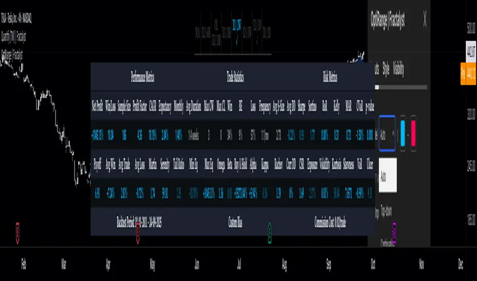
Price Scenarios - The Quant ScienceGENERAL OVERVIEW
Price Scenarios - The Quant Science is a quantitative statistical indicator that provides a forecast probability about future prices moving using the mathematical-statistical formula of statistical probability and expected value.
HOW TO USE
The indicator displays arrow-shaped signals that represent the probable future price movement calculated by the indicator, including the current percentage probability. Additionally, the candlesticks are colored based on the predicted direction to facilitate visual analysis. By default, green is used for bullish movements and red for bearish movements. The trader can set the analysis period (default value is 200) and the percentage threshold of probability to consider (default value is greater than 0.50 or 50%) through the user interface.
USER INTERFACE
Lenght analysis: with this features you can handle the length of the dataset to be used for estimating statistical probabilities.
Expected value: with this feature you can handle the threshold of the expected value to filter, only probabilities greater than this threshold will be considered by the model. By default, it is set to 0.50, which is equivalent to 50%.
Design Settings: modify the colors of your indicator with just a few clicks by managing this function.
We recommend disabling 'Wick' and 'Border' from the settings panel for a smoother and more efficient user experience.
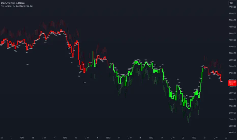
Rolling VWAP [QuantraSystems]Rolling VWAP
Introduction
The Rolling VWAP (R͜͡oll-VWAP) indicator modernizes the traditional VWAP by recalculating continuously on a rolling window, making it adept at pinpointing market trends and breakout points.
Its dual functionality includes both the dynamic rolling VWAP and a customizable anchored VWAP, enhanced by color-coded visual cues, thereby offering traders valuable flexibility and insight for their market analysis.
Legend
In the Image you can see the BTCUSD 1D Chart with the R͜͡oll-VWAP overlay.
You can see the individually activatable Standard Deviation (SD) Bands and the main VWAP Line.
It also features a Trend Signal which is deactivated by default and can be enabled if required.
Furthermore you can find the coloring of the VWAP line to represent the Trend.
In this case the trend itself is defined as:
Close being greater than the VWAP line -> Uptrend
Close below the VWAP line -> Downtrend
Notes
The R͜͡oll-VWAP can be used in a variety of ways.
Volatility adjusted expected range
This aims to identify in which range the asset is likely to move - according to the historical values the SD Bands are calculated and thus their according probabilities displayed.
Trend analysis
Trending above or below the VWAP shows up or down trends accordingly.
S/R Levels
Based on the probability distribution the 2. SD often works as a Resistance level and either mid line or 1. SD lines can act as S/R levels
Unsustainable levels
Based on the probability distributions a SD level of beyond 2.5, especially 3 and higher is hit very seldom and highly unsustainable.
This can either mean a mean reversion state or a momentum slowdown is necessary to get back to a sustainable level.
Please note that we always advise to find more confluence by additional indicators.
Traders are encouraged to test and determine the most suitable settings for their specific trading strategies and timeframes.
Methodology
The R͜͡oll-VWAP is based on the inbuilt TV VWAP.
It expands upon the limitations of having an anchored timeframe and thus a limited data set that is being reset constantly.
Instead we have integrated a rolling nature that continuously calculates the VWAP over a customizable lookback.
To also keep the base utility it is possible to use the anchored timeframes as well.
Furthermore the visualization has been improved and we added the coloring of the main VWAP line according to the Trend as stated above.
The applicable Trend signals are also part of that.
The parameter settings and also the visualizations allow for ample customizations by the trader.
For questions or recommendations, please feel free to seek contact in the comments.
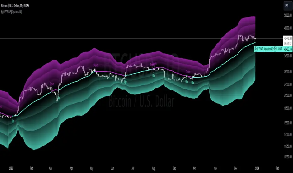
Probability Box Rule of Thirds [PPI]█ Probability Box Rule of Thirds
The Probability Box Rule of Thirds , is a visual indicator that helps traders identify possible overbought and oversold conditions. It does this by dividing the price range – highest high minus the lowest low of a given lookback period or date range – into thirds. Each third has distinct probability characteristics and when combined represent a probability box.
We have spent years refining the probability box concept, and have previously published a How To on Trading View – "How to Trade Probability Ranges – The Critical Rule of 1/3" which can be found here:
To quickly summarize the How To – when using the Rule of Thirds , you are using a combination of statistics, probabilities of success, and prior price action to determine when to enter a trade. The visual range division helps remove subjectivity and clearly shows when the trading odds are stacked in your favor. By identifying and taking higher probability trades, you have a higher chance of success as trading is all about probability and risk management.
Implementing the Rule of Thirds starts with finding an instrument that is consolidating and identifying the nearest important support and resistance levels based on your targeted trading timeframe or lookback period.
The range between the support and resistance levels is divided into thirds to form three zones within the consolidation range.
When going LONG , you want to BUY in the bottom third of the range. Once you buy, your objective is to hold during the middle third and sell when the price enters the top third.
When you buy in the lower third, there's a 66.6% probability of success. If you buy in the middle third, you only have a 50% / 50% chance of success. Going long in the top third of the range gives you a 33.3% chance of success as you are already close to the identified resistance level.
When going SHORT , the sequence and odds are reversed. You want to SELL in the top third of the range, hold the middle third and exit in the bottom third of the range. This gives you a 66.6% chance of success when entering in the top third, a 50% / 50% chance when entering in the middle third, and a 33.3% chance in the bottom third given you are already close to the identified support level.
When the price lies in the middle third, the even 50% / 50% odds provide no probability edge and a trader is better off waiting until the price reaches the upper or lower thirds of the price range.
The Rule of Thirds allows us to quickly visually evaluate trades based on probabilities, selectively enter trades that have the highest odds of success, and avoid likely losing trades. The Rule of Thirds gives you confidence to hold trades based on prior trading ranges and provides clear levels where the prices are likely to either reverse or start trending.
The Probability Box Rule of Thirds automatically implements the first two steps of the Rule of Thirds by using the highest high and lowest low of a given lookback period to identify the support and resistance levels, and automatically divides the range into thirds. The rest of the Rule of Thirds rules remain the same.
Just having the price within the bottom thirds or top thirds, however, does not mean the price will immediately reverse. The GE chart below is an example of a stock that remained 'stuck' in the upper thirds of the price range for an extended amount of time:
And the CVS chart below is an example where the price is 'stuck' in the lower thirds of the price range:
While the price is in the upper or lower thirds, it is very important that the trader should use other indicators to identify when a significant trend reversal occurs. Once a trend reversal event happens, the trader either enters a trade AND/OR exits a trade if already in one.
When the price exceeds the bounds of the probability box, there are three possible outcomes – a strong continuation trend, the price consolidates around the probability box edge, or a trend reversal. Your favorite indicators will help determine which event is happening.
The CVS chart above is a good example of the probability box being exceeded with the last bar. The price exceeding the price range is temporary event as the price range will expand to encompass the revised price range on the next trading day.
█ Indicator Features
Each supported timeframe – Monthly, Weekly, and Daily – allows the selection of an appropriate lookback period for your trading style. The defaults are a good starting point for swing trading and long-term investing. You many need to experiment to find the optimal lookback period for your trading style.
Even if you only day trade, the Probability Box Rule of Thirds with the appropriate lookback periods can help you visualize the bigger picture of where the instrument is heading.
When viewing the charts, you can find the currently selected lookback period above the upper edge of the price range.
The indicator will display a dotted yellow line at 50% of the price range and show the line's value when requested.
The visibility of the actual thirds and border price values are controlled by the " Show Probability Box Values " checkbox. You may need to expand the chart's right margin to see the values.
The " Show Internal Labels " checkbox controls the display of the internal ⅓ Division labels and the percentage odds, along with the 50% label. This option by default is set to off.
The " Show Error Messages " checkbox controls the display of error messages and by default is turned on. Turn off to prevent error messages from being shown on intraday timeframes. Save as indicator default to prevent having to turn off this setting each time added to chart.
The color and transparency controls allow the user to modify the colors used for each third. The default settings are optimized for use with a DARK background.
█ Implementation Notes
IMPORTANT - the Probability Box Rule of Thirds is set up to only handle Monthly, Weekly and Daily charts. This is intentional as the indicator is designed to be used for safer multiple day and longer swing trades. When viewed on intraday charts, the indicator will be hidden.
The Probability Box Rule of Thirds uses a rolling window of the equivalent number of bars for the lookback period rather than relying on the bar starting and ending dates. This allows the use of a standard number of days in the selected lookback window across various instruments and ensures fast, efficient calculations.
The lookback periods are adjusted when non-standard timeframe multipliers are used – e.g., a 12M chart timeframe and a 3-year lookback period will result in a 3 bar lookback. Fractional bars in this calculation are rounded up and any incompatible lookback period and chart timeframe combination will generate a runtime error.
In summary, the Probability Box Rule of Thirds automates and visually identifies overbought and oversold areas, which combined with the Rule of Thirds probability risk profiles, increases your odds of success through better trade selections and higher confidence in your trades.
█ Disclaimer
There is substantial risk in trading. Losses incurred in trading can be significant. Only trade with money you can afford to lose. We make no claims whatsoever regarding the impact of past or future performance on your trading results.
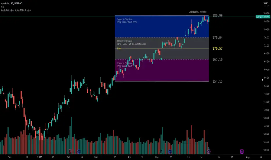
Probability Trend IndicatorUnderstanding the Indicator:
The indicator calculates the probabilities of upward and downward trends based on the percentage change in price over a specified lookback period.
It displays these probabilities in a table and plots a histogram to represent the difference between the probabilities.
The colors of the histogram bars indicate the trend direction and whether the trend is increasing or decreasing.
Setting the Lookback Period:
The indicator allows you to specify the lookback period, which determines the number of bars to consider for calculating the probabilities.
By default, the lookback period is set to 50 bars. However, you can adjust it based on your trading preferences and the timeframe you're analyzing.
Analyzing the Probabilities:
The indicator calculates the probabilities of upward and downward trends and displays them in a table on the chart.
The probabilities are presented as percentages, representing the likelihood of each type of trend occurring.
You can use these probabilities to gain insights into the potential market direction and assess the strength of the prevailing trend.
Interpreting the Histogram:
The histogram is plotted based on the difference between the probabilities of upward and downward trends, known as the oscillator value.
The histogram bars are colored to provide visual cues about the trend direction and whether the trend is gaining or losing strength.
Green bars indicate upward trends, and red bars indicate downward trends.
Lighter shades of green or red suggest increasing trends, while darker shades suggest decreasing trends.
Making Trading Decisions:
The indicator serves as a tool for assessing the probabilities of trends and can be used alongside other technical analysis methods.
You can consider the probabilities, the histogram pattern, and the overall market context to make informed trading decisions.
It's important to remember that no indicator or tool can guarantee future market movements, so prudent risk management and additional analysis are essential.

SFC Smart Money - VolatilityIn statistics, a normal distribution is a type of continuous probability distribution for a real-valued random variable. Normal distributions are important in statistics and are often used in the natural and social sciences to represent real-valued random variables whose distributions are not known.
The indicator provide a deep statistic for the specified period. It calculate the normal distribution of all candles in the particular period, in order to measure the volatility and the probabilities. Also it separate bull from bear candles and calculate the normal distribution of each group. The calculations are mode based on open-open data and high-low data.
Volatility
Volatility is a statistical measure of the dispersion of returns for a given security or market index. In most cases, the higher the volatility , the riskier the security. Volatility is often measured from either the standard deviation or variance between returns from that same security or market index.
Volatility often refers to the amount of uncertainty or risk related to the size of changes in a security's value. A higher volatility means that a security's value can potentially be spread out over a larger range of values. This means that the price of the security can change dramatically over a short time period in either direction. A lower volatility means that a security's value does not fluctuate dramatically, and tends to be more steady.
While variance captures the dispersion of returns around the mean of an asset in general, volatility is a measure of that variance bounded by a specific period of time. Thus, we can report daily volatility , weekly, monthly, or annualized volatility .
This statistic gives very accurate information how the price moved in the past and what are normal movements and spikes. From this information, a future actions can be taken.
For better understanding, all data is calculated in pips.
Features:
- Mean - Mean is the one we are most used to, i.e. the average.
- Median -Sometimes, the data set values can have a few values which are at the extreme ends, and this might cause the mean of the data set to portray an incorrect picture.
Thus, we use the median, which gives the middle value of the sorted data set.
- Mode - In a given dataset, the mode will be the number which is occurring the most.
- Max - Maximum volatility for a given range.
- Min - Minimum volatility for a given range.
- Standard Deviation - The standard deviation tells us how far the value deviates from the mean.
- Range - Range simply gives the difference between the min and max values of the data set.
- ATR - Average True Range measures volatility, taking into account any gaps in the price movement.
- Normal Distribution - The basic premise is that given a range of observations, it is found that most of the values center around the mean and within one standard deviation
away from the mean.
- Probability - probability of outcomes.
We all know that the banks and professional traders do not trade with charts, but with different statistical methods, math. models and macroeconomics. This statistical indicator shows one of these methods.
It is recommended to use the indicator on daily timeframe . It also works on other timeframes, for example 1H for intraday analysis.
For more information how the normal distribution works, please search in internet.

Reinforced RSI - The Quant Science This strategy was designed and written with the goal of showing and motivating the community how to integrate our 'Probabilities' module with their own script.
We have recreated one of the simplest strategies used by many traders. The strategy only trades long and uses the overbought and oversold levels on the RSI indicator.
We added stop losses and take profits to offer more dynamism to the strategy. Then the 'Probabilities' module was integrated to create a probabilistic reinforcement on each trade.
Specifically, each trade is executed, only if the past probabilities of making a profitable trade is greater than or equal to 51%. This greatly increased the performance of the strategy by avoiding possible bad trades.
The backtesting was calculated on the NASDAQ:TSLA , on 15 minutes timeframe.
The strategy works on Tesla using the following parameters:
1. Lenght: 13
2. Oversold: 40
3. Overbought: 70
4. Lookback: 50
5. Take profit: 3%
6. Stop loss: 3%
Time period: January 2021 to date.
Our Probabilities Module, used in the strategy example:

Probabilities Module - The Quant Science This module can be integrate in your code strategy or indicator and will help you to calculate the percentage probability on specific event inside your strategy. The main goal is improve and simplify the workflow if you are trying to build a quantitative strategy or indicator based on statistics or reinforcement model.
Logic
The script made a simulation inside your code based on a single event. For single event mean a trading logic composed by three different objects: entry, take profit, stop loss.
The script scrape in the past through a look back function and return the positive percentage probability about the positive event inside the data sample. In this way you are able to understand and calculate how many time (in percentage term) the conditions inside the single event are positive, helping to create your statistical edge.
You can adjust the look back period in you user interface.
How can set up the module for your use case
At the top of the script you can find:
1. entry_condition : replace the default condition with your specific entry condition.
2. TPcondition_exit : replace the default condition with your specific take profit condition.
3. SLcondition_exit : replace the default condition with your specific stop loss condition.

Divergence Backtester - V2Further attempts to study divergence impact on price in shorter terms.
Previous study can be found here:
In this script, we are trying to gather the stats based on last two pivot state together. For example, Individual table of Pivot High Projection is as explained below:
But, by looking at the bigger picture, we can further estimate following things regarding the current unconfirmed pivot and the new pivot which is yet to be formed.

Probabilistic Analysis Table - The Quant ScienceProbabilistic Analysis Table - The Quant Science ™ is the quantitative table measuring the probability of price changes and quantifies the ratio of sessions for three different assets.
This table measures the ratios of bull and bear events and measures the probability of each event through data generated automatically by the algorithm.
The data are calculated for three different assets:
1. Main asset: set on the chart.
2. Second asset: set by user interface.
3. Third asset: set by the user interface.
The timeframe is set by the chart and is the same for all three assets. You can change the timeframes directly from the chart.
The user can add tickers and adjust the analysis period directly from the user interface. The user can edit the percentage changes and the values to be analyzed for each asset, directly from the user interface.
TABLE DESCRIPTION
1. Total global trade session: are the total number of bars for each asset.
2. Total positive trade session: are the number of positive bars for each asset.
3. Probability positive trade session: is the ratio of total sessions to positive sessions.
4. Total negative trade session: are the number of negative bars for each asset.
5. Probability negative trade session: is the ratio of total sessions to negative sessions.
6. Positive trade session 0.50%: are the number of positive bars greater than 0.50% for each asset.
7. Probability positive trade session 0.50%: is the ratio of total sessions to positive sessions with increases greater than 0.50% (this value is set by default, you can change it from the user interface).
8. Negative trade session -0.50%: are the number of negative bars smaller than -0.50% for each asset.
9. Probability negative trade session -0.50%: is the ratio of total sessions to negative sessions with declines less than -0.50% (this value is set by default, you can change it from the user interface).
10. Positive trade session 1%: are the number of positive bars greater than 1% for each asset.
11. Probability positive trade session 1%: is the ratio of total sessions to positive sessions with increases greater than 1% (this value is set by default, you can change it from the user interface).
12. Negative trade session -1%: are the number of negative bars less than -1% for each asset.
13. Probability negative trade session -1%: is the ratio of total sessions to negative sessions with declines less than -1% (this value is set by default, you can change it from the user interface).
This table was created for traders and quantitative investors who need to quickly analyze session ratios and probabilities.
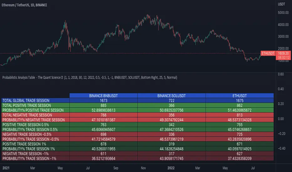
iCryptoScalperHi everyone!
In this post I would like to present my personal indicator for short-term strategies on cryptocurrencies called iCryptoScalper , but let me first introduce myself:
I am a theoretical physicist with a deep passion for trading and mathematical modelling of the financial markets.
I started trading cryptocurrencies more than 4 years ago and, throughout this period, I got more and more involved in trying to describe the mechanisms governing
the price action at lower timeframes like 1, 5 and 15 minutes.
As a beginner, I started with the usual "buy and hold" strategy, the safest but also boring option. Afterthat, I tried to get more involved on speed trading
and scalping and, as it happens to all the beginners, I went through many mistakes.
At the beginning, trying to find the best scalping strategy, was a very difficult task and I barely managed to perform well, mostly because every trade were overwhelmed
by my emotional approach and the fear of missing the right entry point and/or exit point. However, thanks to these difficulties, I understood that I needed
an algorithmic procedure to improve my performances and overtake the emotional approach, with a more technical approach: a mathematical guide that precisely tells me how to behave in the best way possible to be profitable.
To achieve this goal, I put all my efforts in trying to write a consistent mathematical model able to give me all the statistical informations I needed to reach
the best performances and, of course, the best possible profits.
The iCryptoScalper is an explicit mathematical tool to be used for scalping strategies and optimized for different cryptocurrency pairs on 15/30 min timeframes.
The script gives you many useful informations and details regarding the current and subsequent trade, accompanied with a detailed overview on both the last 20 short
and long trade results.
Let us have a look to all the detailed informations the script shows to you:
CHART
- Lines: The script plots for you the Entry price (yellow line), the Stop Loss price (red line) and a series of 8 Take Profit levels (green lines).
- Background: The green background color indicates that the script is in a long position, viceversa, the red background color indicates that the script is in a short position.
- Labels: The blue labels indicate the maximum achieved profit for each trade.
- Alerts: The script shows two types of alerts, the "prepare to #" one and the true entry one. The prepare alert is very useful to understand when the strategy is going
to enter a specific trade, thus giving you the possibility to set up all the necessary Entry/SL/TP levels on your favorite trading platform.
- Crosses: The green and red crosses are precisely located at the corresponding long and short entry price for the next trade, thus giving you a preview on the target price
that has to be reached for the indicator to enter. They are computed thanks to a mathematical model I set up and optimized for each cryptocurrency pair.
PANEL
- Overview: This part shows you two probability tables for the last 20 long and short trades each. The first table indicates the set of probabilities of reaching the corresponding TP level, whereas the second table shows the conditional probability , namely the probability of reaching a certain profit level once the previous one has been achieved.
Below the tables you can find three quantities again referring to the last 20 long and short trades: the Average Maximum Profit , the Average Maximum Drawdown and the Average Risk/Reward Ratio .
Last but not least, the correlation between the current asset and BTC is displayed together with the current BTC status.
- Active Trade: This part collects all the data related to the current trade status.
- Next Trade: This part collects all the data related to the next trade status.
ATTENTION!
Please notice that the equity line you see in the "Strategy Tester" section of TradingView is unreliable compared to the real performances of the script. This is due to the
fact that the TradingView engine is designed for backtesting automatic trading strategies and not real-time trading bots.
An example is the following: Bob buys 1 BTC-PERP contract at 10000$, setting the Stop Loss at 9000$. The price of the perpetual then goes to 12000$ and then go back hitting the Stop Loss. For the TradingView Engine this is a
trade with a permanent loss of 1000$. However, for the iCryptoScalper users, the trade is perfectly fine thanks to the numerous TP levels (and corresponding probabilities) given by the script within the trade window.
Chobotaru IndicatorChobotaru Indicator has two functions:
1. Probability cloud, giving the probability of stock or future to move to a certain price.
2. Help traders understand where to take profit and where to put a stop-loss.
You don’t need knowledge about options trading, this indicator is for all traders/investors.
What does the indicator do?
The indicator is based on the partial differential equations from the mathematical model of options, the Black-Scholes model. Using these equations and market parameters the indicator shows on the chart the probability that the stock/future will touch a certain price until a specific date.
How the indicator does it?
The algorithm solves the partial differential equations using the following values:
Instrument price - The current price of the stock or futures contract
The interest rate – default zero – can be found by searching in google: “U.S. Department of the treasury daily yield curve rates”, Use the 3-month value. This value has a low impact on the model so you only need to update it when there is a major change in the percentile. (Example, in January 2021 the 3 months “risk-free rate” is 0.08, you can enter 0 in the indicator.
Days to expire (minus trading holidays) – You need to choose an option and take from it the other values that are needed. We recommend taking options that close to 30 days, but it is the user choice.
Example: On the 22 of January 2021, PLTR has an option that has 35 days left. The option will expire on the 26 of February 2021, if there are trading holidays like in this case, the user needs to subtract them, on the 15 of February we have Washington's Birthday, the input is 35-1=34.
Implied volatility - Annualized asset price volatility, specific as a positive decimal number. IV 10% => input 0.1, you can find it in the option chain, if you don’t know what it is, you can ask your broker where you can find it on your trading platform. For example, the IV of PLTR on the 22 of January 2021 is 120.67% the input is 1.2067
Date – Entering the date of entry.
How the indicator helps traders and how to use it?
After you enter the inputs correctly, you will see colorful lines, each line representing the probability for the price to touch there in the current market conditions until a specific date.
To see what percentage each color represents in the indicator press “style”. For example, red lines are a 50% chance for the price to touch there in the chosen period.
It also helps the trader to see what range the stock is expected to move and what range is not probable in this period (according to the options prices).
As you can see, the probability cloud is expanding. This is because as time passes, the probabilities of reaching far away prices are increasing.
How to access the indicator?
Use the link below to obtain access to the indicator
Note: this indicator may not work on IPO

Bayesian BBSMA OscillatorSometime ago (very long ago), one of my tinkering project was to do a spam or ham classification type app to filter news I'd wanna read. So I built myself a Naive Bayes Classifier to feed me my relevant articles. It worked great, I can cut through the noise.
The hassle was I needed to manually train it to understand what I wanna read. I trained it using 50 articles and to my surprise, it's enough.
Complexity Theory
I've been reading a book called The Road to Ruin by Jim Rickards. He described how he got to his conclusion of how the stock market works by using Complexity Theory. Bill Williams would agree. Jim tells us that by using just enough data, we calculate the probability of an event to occur. We can't say for sure when but we know it's coming. This was my light bulb moment.
While Jim talks much about Bayesian Inference in which a probability of an event can always be updated as more evidence comes to light, I had my eyes set on binary probabilities of when prices are going up and down.
Assumptions
These are my assumptions:
Prices breaking up a Bollinger basis line will have fuel to go up even higher
Prices will go down when prices have broken up a Bollinger upper band
Scalping is the main method so we should use a lower period Moving Average (MA)
When prices are above MA, it's likelier a correction to the downside is imminent
When prices are below MA, it's likelier a correction to the upside is imminent
Optimize parameters for 1 hour timeframe which will give us time to react while still having more opportunities to trade
Building Blocks
Jim Rickards started with limited data (events) while in technical trading, data are plentiful. I decided to classify 2 events which are:
Next candles would be breaking up
Next candles would be breaking down
Key facts:
We won't know for sure when prices are going to break
We won't know for sure how much the prices movements are going to be
Formulas
Breaking up:
Pr(Up|Indicator) = Pr(Indicator|Up) * Pr(Up) / Pr(Indicator|Up) * Pr(Up) + Pr(Indicator|Down) * Pr(Down)
Breaking down:
Pr(Down|Indicator) = Pr(Indicator|Down) * Pr(Down) / Pr(Indicator|Down) * Pr(Down) + Pr(Indicator|Up) * Pr(Up)
Reading The Oscillator
Green is the probability of prices breaking up
Red is the probability of prices breaking down
When either green or red is flatlining ceiling, immediately on the next candle when the probability decreases go short or long based on which direction you're observing - Strong Signal
When either green or red is flatlining ceiling, take no action while it's ceiled
Usually when either green or red is flatlining bottom, the next candle when the probability increases, immediately take a short long position based on the direction you're observing - Weak Signal
When either green or red is flatlining bottom, take no action while it's bottomed
Alerts
Use Once per Bar option when generating alerts.
