Crypto PCA [LuxAlgo]The Crypto PCA indicator provides a sophisticated, multi-asset sentiment gauge by applying Principal Component Analysis (PCA) to a basket of the top 20 cryptocurrencies.
By extracting the primary driver of variance across these assets, the tool offers a "market-wide" oscillator that filters out individual coin noise to highlight the dominant trend and sentiment shifts in the crypto space.
In modern quantitative finance, PCA is used to reduce dimensionality and identify the underlying factors that move a group of assets. This indicator brings that institutional-grade approach to the retail trader, condensing the price action of Bitcoin, Ethereum, Solana, and 17 other majors into a single, actionable signal.
🔶 USAGE
The script serves as a macro-sentiment oscillator, allowing traders to see the "hidden" force driving the crypto market. It is designed to identify when the market is moving in unison and when that collective movement has reached an extreme.
🔹 Identifying Market Regimes
The primary use of the PCA line (PC1) is to determine the current market regime. When the oscillator is above the zero line and colored green, it indicates that the majority of the top 20 assets are experiencing positive variance, signaling a broad bullish regime. Conversely, when the line is below zero and colored red, the market is in a collective bearish state. Traders can use this to align their individual trades with the direction of the total market energy.
🔹 Using Snapshot Mode for Situational Analysis
While the continuous mode is ideal for long-term trend following, the Snapshot Mode provides a focused view of market dynamics over the most recent lookback window. This mode isolates the current sentiment cycle, allowing traders to see the specific trajectory and "shape" of the latest move without the influence of older historical data.
By enabling Snapshot Mode, you can analyze the immediate internal structure of the market. It is particularly useful for identifying whether a recent pump or dump is a coordinated market-wide event or a more fragmented move. This helps in distinguishing between a broad structural shift and a temporary volatility spike.
🔹 Spotting Overextended Sentiment
The indicator includes dashed horizontal lines at +2 and -2, representing standard deviation thresholds. Because the assets are standardized before calculation, these levels mark statistical extremes.
Overbought Extremes: When the PCA line exceeds +2, the broad market is significantly overextended to the upside. This often precedes a cooling-off period or a mean-reversion event across the entire sector.
Oversold Extremes: When the PCA line drops below -2, it suggests a "panic" or exhausted selling state across the basket. This can signal potential bottoming interest or a relief rally.
🔹 Gauging Relative Strength
The faint "ghost" lines in the background represent the individual standardized price paths of the 20 included assets. By comparing these to the main PCA line, traders can identify leaders and laggards. An asset line that stays consistently above the PCA line during a rally is exhibiting relative strength, while an asset trailing below the PCA line is underperforming the market average.
🔶 DETAILS
The indicator follows a rigorous mathematical pipeline to ensure the data is statistically significant and comparable across assets with different price scales.
🔹 Standardization (Z-Scores)
Before performing PCA, every asset must be on the same scale. The script converts the price of all 20 assets into Z-scores based on the user-defined Lookback Period. A Z-score tells us how many standard deviations a price is from its mean. This allows the movement of a high-priced asset like BTC to be mathematically compared to a lower-priced asset like PEPE.
🔹 The Basket & PCA Approximation
The indicator includes the following assets: BTC, ETH, BNB, XRP, SOL, TRX, DOGE, ADA, BCH, WBTC, XLM, LTC, HBAR, LINK, AVAX, PEPE, DOT, UNI, NEAR, and ICP.
The script uses a correlation-based approximation to find the First Principal Component. It calculates the correlation of each asset to the equally weighted basket and uses these correlations as "loadings" to compute the PC1. This ensures that assets moving in sync with the general market trend are given higher priority in the final oscillator value.
🔹 Why PCA?
Most "Crypto Indices" are simply weighted averages. PCA is superior because it identifies the commonality between assets. If 18 coins are moving up and 2 are moving down, PCA gives more weight to the 18 moving together, as they represent the "Principal Component" of the market's current energy.
🔶 SETTINGS
🔹 Main Settings
Lookback Period (N): Determines the window used for Z-score standardization and PCA calculation. A shorter period makes the indicator more reactive, while a longer period identifies macro-cycle shifts.
Z-Score Smoothing: Applies a Simple Moving Average (SMA) to the standardized asset values before the PCA calculation. This effectively filters out high-frequency noise and produces a smoother principal component line, which is useful for reducing false regime shifts in volatile markets.
Enable Snapshot Mode: Switches the visual output from a continuous rolling line to a static view of the PCA over the most recent lookback window.
🔹 Visual Settings
Standardized Assets Color: Controls the color and transparency of the 20 individual asset lines.
Bull/Bear Colors: Defines the colors used for positive and negative market sentiment.
Disclaimer: This indicator is a statistical tool for sentiment analysis and does not constitute financial advice. The PCA approach measures variance and correlation, not guaranteed future direction.
Crypto

Smart money PSP with color themesPSP with Color Themes — Price Strength Parity Indicator
PSP with Color Themes is a visual correlation indicator designed to detect Price Strength Parity (PSP) between the current chart symbol and a reference symbol.
It highlights candles where price behavior between two correlated instruments diverges or aligns, which is often used in SMT (Smart Money Technique) and intermarket analysis.
The indicator works directly on the chart and colors candles when a PSP condition is detected, using flexible and customizable color themes.
📌 What Is PSP (Price Strength Parity)?
PSP identifies situations where two correlated assets:
Move in opposite directions → Direct PSP (classic SMT divergence)
Move in the same direction → Inverse PSP (confirmation mode)
Such behavior often precedes:
Reversals
Continuations
Liquidity grabs
Market structure shifts
⚙️ Indicator Inputs
Reference Symbol
Defines the second asset used for comparison (e.g., ETHUSDT vs BTCUSDT).
Purpose:
To detect relative strength or weakness between two correlated markets.
Inverse Correlation Mode
Inverse Correlation Mode (true / false)
Allows switching between divergence-based and confirmation-based analysis.
Color Theme
Available presets:
Green / Red
Blue / Orange
Purple / Yellow
Teal / Pink
Custom
Purpose:
Adapts the indicator visually to different chart styles and backgrounds.
📈 How to Use in Trading
Typical use cases:
SMT divergence detection
Intermarket confirmation
Reversal timing
Liquidity sweep context
SMC / ICT models
Recommended combinations:
Market Structure (BOS / CHoCH)
Fair Value Gaps
Liquidity levels
Session highs /lows
⚠️ Important Notes
PSP is context-based, not a standalone entry system
Best results on correlated markets:
BTC / ETH
Indices (ES / NQ / YM)
FX pairs (EURUSD / DXY)

Session Liquidity Reversion Strategy (Asia Range False Breakout)Overview
This strategy is based on a session-driven liquidity hypothesis rather than a simple indicator combination.
During the Asian trading session, many markets enter a low-liquidity equilibrium, forming a relatively narrow price range. When higher-volume participants enter during the London and New York sessions, price often performs false expansions beyond this Asian range before reverting back toward fair value.
This script systematically identifies and trades those failed session expansions.
Core Concept
The strategy operates in three distinct phases:
Asia Session Range Formation
The high and low of the Asian session are recorded.
This range represents a temporary balance area formed under reduced participation.
Range Locking
Once the Asian session ends, the range is frozen.
No repainting or forward-looking calculations are used.
False Breakout Detection & Reversion
During the London/New York session, price must break beyond the Asia range and fail to hold.
A momentum filter (RSI) confirms rejection strength.
Trades are entered only after price closes back inside the range, targeting reversion rather than continuation.
This approach avoids chasing breakouts and instead focuses on liquidity traps and failed expansions.
Risk Management & Assumptions
Risk parameters are intentionally conservative and realistic:
Position sizing uses percentage of equity
Default risk per trade is approximately 2%
Stop losses are ATR-based, adapting to volatility
Risk-to-reward is fixed and configurable
Realistic commission and slippage are included
One trade per session is allowed to avoid over-exposure
No martingale, grid, or averaging logic is used.
Usage Notes
Recommended timeframes: 5m – 30m
Designed for: Forex, Indices, Crypto
Performance will vary by instrument and session volatility
All parameters are configurable for research and optimization
This strategy is intended for educational and research purposes, demonstrating how session-based liquidity behavior can be tested systematically using Pine Script.

Smart Money Structure FilterEnglish Description
Overview
Smart Money Structure Analyzer is a professional trading tool that implements Smart Money Concepts (SMC) to identify key market structure shifts, Break of Structure (BOS), and Change of Character (CHoCH) patterns. This indicator helps traders follow the "smart money" flow by detecting institutional order flow patterns on any timeframe.
Key Features
Swing Point Detection - Identifies significant highs and lows using fractal-based logic
Market Structure Analysis - Classifies market conditions as Uptrend, Downtrend, or Consolidation
Break of Structure (BOS) - Detects when price breaks key structural levels
Change of Character (CHoCH) - Identifies potential trend reversals
Mitigation Levels - Shows potential retracement targets after structure breaks
How It Works
The indicator analyzes price action through several layers:
Swing Detection Algorithm
Uses a configurable swing period (3-21 bars)
Identifies valid swing highs and lows that are confirmed by surrounding price action
Stores the last 20 swings for structure analysis
Structure Determination
Uptrend: Higher Highs (HH) + Higher Lows (HL)
Downtrend: Lower Lows (LL) + Lower Highs (LH)
Consolidation: Mixed structure or ranging market
Break of Structure (BOS) Logic
Bearish BOS: Price closes below the last confirmed Higher Low (HL)
Bullish BOS: Price closes above the last confirmed Lower High (LH)
Change of Character (CHoCH) Logic
Bearish CHoCH: After a bearish BOS, price forms a Lower Low (confirms trend reversal)
Bullish CHoCH: After a bullish BOS, price forms a Higher High (confirms trend reversal)
Mitigation Levels
Calculates potential retracement levels after BOS (typically ±0.2% from broken structure)
Visual Elements
Fractals: Swing points (optional display)
Structure Lines: Last Higher Low (blue) and Last Lower High (purple)
BOS Signals: Triangles marking structure breaks
CHoCH Signals: Circles confirming trend changes
Mitigation Levels: Dotted orange lines for potential retracements
Info Label: Real-time structure status and key levels
Alerts
The indicator provides alerts for:
Break of Structure (BOS) events
Change of Character (CHoCH) confirmations
Settings
Swing Period: Sensitivity of swing detection (default: 3)
Show Fractals: Toggle swing point markers
Show Structure Lines: Display key structure levels
Show Break of Structure: Display BOS signals
Show Change of Character: Display CHoCH signals
Show Mitigation Levels: Display retracement levels
Best Practices
Use on higher timeframes (1H+) for more reliable signals
Combine with volume analysis for confirmation
Wait for CHoCH confirmation before entering trades
Use mitigation levels as potential entry zones
Русское описание
Обзор
Smart Money Structure Analyzer - профессиональный торговый инструмент, реализующий концепции Smart Money (SMC) для определения ключевых сдвигов рыночной структуры, Break of Structure (BOS) и Change of Character (CHoCH). Индикатор помогает отслеживать поток "умных денег", выявляя паттерны институционального ордерного потока на любом таймфрейме.
Ключевые возможности
Определение свингов - Выявляет значимые максимумы и минимумы с помощью фрактальной логики
Анализ структуры рынка - Классифицирует состояние рынка: Восходящий тренд, Нисходящий тренд или Консолидация
Break of Structure (BOS) - Обнаружение пробития ключевых уровней структуры
Change of Character (CHoCH) - Определение потенциальных разворотов тренда
Уровни митигации - Показывает потенциальные цели отката после пробоя структуры
Принцип работы
Индикатор анализирует ценовое действие через несколько уровней:
Алгоритм определения свингов
Использует настраиваемый период свинга (3-21 свечи)
Определяет валидные максимумы и минимумы, подтвержденные окружающим движением цены
Сохраняет последние 20 свингов для анализа структуры
Определение структуры
Восходящий тренд: Higher Highs (HH) + Higher Lows (HL)
Нисходящий тренд: Lower Lows (LL) + Lower Highs (LH)
Консолидация: Смешанная структура или флет
Логика Break of Structure (BOS)
Медвежий BOS: Цена закрывается ниже последнего Higher Low (HL)
Бычий BOS: Цена закрывается выше последнего Lower High (LH)
Логика Change of Character (CHoCH)
Медвежий CHoCH: После медвежьего BOS формируется Lower Low (подтверждает разворот)
Бычий CHoCH: После бычьего BOS формируется Higher High (подтверждает разворот)
Уровни митигации
Расчет потенциальных уровней отката после BOS (обычно ±0.2% от сломанной структуры)
Визуальные элементы
Фракталы: Точки свингов (опционально)
Линии структуры: Последний Higher Low (синий) и последний Lower High (фиолетовый)
Сигналы BOS: Треугольники, отмечающие пробой структуры
Сигналы CHoCH: Круги, подтверждающие изменение тренда
Уровни митигации: Пунктирные оранжевые линии для потенциальных откатов
Инфо-метка: Статус структуры и ключевые уровни в реальном времени
Оповещения
Индикатор предоставляет алерты для:
Событий Break of Structure (BOS)
Подтверждений Change of Character (CHoCH)
Настройки
Период свинга: Чувствительность определения свингов (по умолчанию: 3)
Показывать фракталы: Включение/выключение маркеров свингов
Показывать линии структуры: Отображение ключевых уровней структуры
Показывать Break of Structure: Отображение сигналов BOS
Показывать Change of Character: Отображение сигналов CHoCH
Показывать уровни митигации: Отображение уровней отката
Рекомендации по использованию
Используйте на старших таймфреймах (1H+) для более надежных сигналов
Комбинируйте с анализом объема для подтверждения
Ждите подтверждения CHoCH перед входом в сделку
Используйте уровни митигации как потенциальные зоны входа
Технические особенности
Максимальное количество меток: 500
Работает на любых таймфреймах
Не перерисовывает прошлые сигналы
Эффективно использует ресурсы благодаря ограничению хранения свингов
Индикатор предназначен для трейдеров, работающих с Price Action и концепциями Smart Money, и помогает систематизировать анализ рыночной структуры в соответствии с подходами институциональных трейдеров.

Bitcoin Halving Cycles [DotGain]Halving Cycles
A lightweight, time-anchored Bitcoin halving cycle visualizer built for clean charting, repeatable process planning, and simple profit/DCA timing references.
This Code was heavily inspired by KevinSvenson_ who created Bitcoin Halving Cycle Profit .
What this indicator does
This script plots the key “cycle landmarks” relative to each halving date:
Halving (⛏) – the cycle anchor
Profit START – marks the beginning of the post-halving profit window (default: 40 weeks )
Profit END / Last Call – marks the final phase of the profit window (default: 77 weeks )
DCA START – marks the point where long-term accumulation becomes the focus again (default: 135 weeks )
How to read it
Vertical lines = the exact cycle milestones
Bottom labels = description of each milestone aligned to its line (keeps the chart clean)
Green background (optional) = active Profit Zone on existing bars
Red background (optional) = optional warning zone after Profit END
HUD Panel (top-right)
The HUD gives you a fast “where are we in the cycle?” view with two modes:
Current Cycle
Shows: Halving date, Weeks since, and time remaining to Profit START / Last Call / DCA START within the current cycle.
Next Halving (Projection)
Shows: Countdown to the next enabled future halving, plus the projected weeks from today to Profit START / Last Call / DCA START after that future halving.
Future Halvings (manual)
You can manually add up to 3 future halving dates (Halving #1–#3).
This is useful for forward planning and cycle projection even before the event happens.
Enable Halving #1 / #2 / #3
Set Year / Month / Day for each
Optional: show/hide future markers & projections
Note: background zones only shade existing bars . Future projections are shown via lines/labels.
Settings overview
Show all cycles – plots every enabled cycle (historical + optional future). If disabled, only the current cycle is drawn.
Show Profit Zone background – green shading during the active profit window (current cycle only).
Show vertical markers + labels – toggles all milestone lines + labels.
Show HUD – toggles the HUD panel.
HUD Mode – switch between Current Cycle and Next Halving (Projection).
Cycle Logic – edit offsets in weeks (Profit START / Profit END / DCA START).
Optional Warning Zone – show a post-profit warning shading for a chosen number of weeks.
Have fun :)
Disclaimer
This Halving Cycles indicator is provided for informational and educational purposes only. It does not, and should not be construed as, financial, investment, or trading advice.
This indicator is an independent implementation of a time-based Bitcoin halving cycle visualization tool and is not affiliated with, or endorsed by, any third-party trading systems, strategies, protocols, or trademarked methodologies. The cycle zones, milestone markers, and countdown values displayed by this indicator are generated by a predefined set of algorithmic rules based on historical halving dates and user-defined time offsets. They do not constitute a direct recommendation to buy, sell, or hold any financial instrument or digital asset.
All trading and investing in financial markets involves a substantial risk of loss. You may lose part or all of your invested capital. Past performance does not guarantee future results. This indicator highlights historical and projected time-based market cycles and may produce false, lagging, incomplete, or misleading signals. Market behavior is influenced by many external factors and can deviate significantly from historical patterns or expectations.
The creator DotGain assumes no responsibility or liability for any financial losses, damages, or decisions made based on the use of this indicator or the information it provides. You are solely responsible for your own trading and investment decisions. Always conduct your own research (DYOR), use proper risk management, validate insights with additional tools or analysis, and consider your personal financial situation and risk tolerance before making any financial decision.

Mission Control Dashboard (AI, Crypto, Liquidity) FASTCONCEPT Price is a lagging indicator. Liquidity is a leading indicator. "Mission Control Dashboard (AI, Crypto, Liquidity) FAST" is a sophisticated macroeconomic dashboard designed to audit the "plumbing" of the financial system in real-time. Unlike standard indicators that rely solely on price action, this tool pulls data from the Federal Reserve (FRED), Treasury Statements, Corporate Financials (10-K/10-Q), and On-Chain Stablecoin metrics to visualize the structural flows driving the market.
THE "UNIFIED FIELD" SOLVER One of the hardest challenges in cross-asset scripting is "Time Dilation"—synchronizing 24/7 Crypto markets (Bitcoin) with Mon-Fri Traditional markets (Stocks/Bonds).
Standard scripts fail on weekends, showing mismatched data.
This engine uses a Weekly Anchor system. It calculates all momentum and liquidity metrics based on "Week-to-Date" or "Month-Ago" anchors. This ensures that a "Liquidity Drain" looks identical whether you are viewing a Bitcoin chart on Saturday or an Apple chart on Monday.
THE CHRONOS LOGIC The dashboard is sorted by Time Sensitivity (Speed of impact), from fast-twitch tactical signals to slow-moving structural fundamentals.
1. TACTICAL (Reacts in 24–48h)
Stablecoin Flight: Measures the immediate flow of capital from Volatile Assets to Stablecoins (USDT/USDC). A spike (>0.5%) indicates fear/sidelining.
Liquidity Alpha: Calculates the efficiency of capital. It subtracts "Friction" (Dollar Strength + Yields) from "Flow" (Liquidity Beta). High Alpha means money is flowing easily into risk assets.
Alt Euphoria: Tracks the overheating of the Altcoin market (TOTAL3). Green indicates sustainable growth; Red (>45%) warns of a "blow-off top."
Retail FOMO: A sentiment gauge comparing Coinbase Stock ( NASDAQ:COIN ) performance vs. Bitcoin ( CRYPTOCAP:BTC ). When Retail outperforms the Asset, local tops often follow.
2. LIQUIDITY & MACRO (Reacts in 1–4 Weeks)
Debt Wall (10Y): The Rate-of-Change of the US 10-Year Treasury Yield. Spiking yields act as gravity on risk assets.
Liquidity Beta: The raw "Quantity of Money." Tracks the 4-week change in Net Liquidity (Fed Balance Sheet - TGA + Stablecoins).
TGA Balance: The Critical Monitor. Tracks the Treasury General Account. When the TGA rises (Red), the government is draining liquidity from the banking system. When it falls (Green), it releases cash.
Note: This script includes an auto-scaler to handle TGA data in both Billions and Millions.
3. STRUCTURAL (Reacts in 3–12 Months)
AI Capex (YoY & QoQ): The "Floor" of the 2025/2026 cycle. Tracks the Capital Expenditure of the Hyperscalers (MSFT, GOOGL, AMZN, META). As long as this remains high (>30%), the infrastructure boom supports the tech narrative.
PMI Manufacturing: Tracks the ISM Manufacturing cycle. Contraction (<50) often forces Fed intervention.
Micron Inventory: A lead indicator for the hardware cycle.
HOW TO USE
Status Colors: The traffic light system helps you assess risk at a glance.
🟢 GREEN (Healthy): Flow is positive, friction is low, fundamentals are strong.
🔴 RED (Danger): Liquidity is draining (TGA spike), yields are shock-rising, or FOMO is excessive.
Zero Configuration: The script auto-detects asset classes and scales units (Billions/Trillions) automatically.
DATA SOURCES
Federal Reserve Economic Data (FRED)
Daily Treasury Statement (DTS)
CryptoCap (TradingView)
Nasdaq/Corporate Financials
Disclaimer: This tool is for informational purposes only and does not constitute financial advice. Macro data feeds are subject to reporting delays.

Mission Control Dashboard (AI, Crypto, Liquidity)Description: Mission Control Dashboard (AI, Liquidity) is a comprehensive macro-liquidity and cycle-analysis dashboard designed to track the "Flow of Funds" across traditional and crypto markets. Instead of looking at price action alone, this script monitors the fundamental "plumbing" of the global economy.
Key Metrics Tracked:
The Debt Wall: Monitors the US 10Y Yield and TLT price. It signals a "Critical" state if yields spike above 5% or TLT drops below $80, indicating high stress in the bond market.
Global Liquidity (MTF Stable): A proprietary calculation summing the balance sheets of the FED, ECB, BoJ, and PBoC, plus Stablecoin market cap. It calculates the Rate of Change (ROC) to see if the world is "printing" or "draining" money.
TGA Hidden Fuel: Tracks the Treasury General Account. A falling TGA is often bullish for risk assets as it injects liquidity into the banking system.
Universal Alt Season: Monitors TOTAL3 (Crypto market cap excluding BTC & ETH) for parabolic moves (>30% ROC).
AI Infra Capex: Real-time tracking of Capital Expenditures from MSFT, GOOG, AMZN, and META to gauge the health of the AI cycle.
How to use:
Green Status across the board: High probability for "Risk-On" environments (Alt season, Tech rallies).
Strategic Beta vs. Tactical Alpha: If Beta is draining but Alpha is accelerating, it suggests a "False Breakout" or a divergence in liquidity.
Uranium Trend: Used as a proxy for the energy transition and long-term industrial cycle strength.

Leswin Ribbon + Levels + Hybrid (Stocks/Crypto) v1Leswin Ribbon Signals
A trend-based momentum indicator built for day traders and scalpers. Uses an EMA ribbon, higher-timeframe trend filtering, and volatility conditions to highlight high-probability BUY and SELL zones while avoiding choppy markets.
Optimized for 5m & 15m entries, especially for SPY, QQQ, DIA, IWM, and large-cap stocks, but works on all markets including crypto and forex.
Non-repainting. Best used as a confirmation tool alongside your own levels and risk management.

Leswin Stocks Ribbon Signals (SPY/QQQ)
Leswin Ribbon Signals – Day Trading Indicator (Stocks & Crypto)
Leswin Ribbon Signals is a trend-based momentum indicator designed for day traders and scalpers who trade stocks, ETFs, options, and crypto.
Built for fast execution on 5m, 15m, and 1H timeframes, it uses a dynamic EMA ribbon, trend filtering, and volatility conditions to help identify high-probability BUY and SELL zones while avoiding low-quality chop.
Features:
• Trend-following EMA ribbon
• Automatic higher-timeframe trend filter
• Smart BUY & SELL signals
• Volatility (ATR) filter to avoid dead zones
• Regular Trading Hours (RTH) filter for stocks
• Optimized for SPY, QQQ, DIA, IWM, TSLA, AAPL, META
• Works on crypto, forex, and futures
• Mobile-friendly
• Non-repainting logic
This indicator is best used as a confirmation tool, not a standalone system. Always combine with your own levels, structure, and risk management.

WEEKEND BOX (FRIDAY 17:00 - SUNDAY 18:00 NY)As the name “Weekend Box” suggests, this indicator highlights the price range of cryptocurrencies between Friday 17:00 and Sunday 18:00 (New York time). It draws a box around this period to visualize how Bitcoin and other crypto assets behave while the forex market is closed. The goal is to provide a simple, educational tool for anyone interested in studying weekend volatility and market behavior in crypto. Thank you.

BTC - Satoshis Altcoin Graveyard OVERVIEW
The Satoshi's Altcoin Graveyard (SAG) is a macro-statistical engine designed to solve the problem of Survivorship Bias . It is a well-known phenomenon in the crypto markets that the "Top 10" list is in a constant state of flux. If you look at historical data from CoinMarketCap (CMC) year by year, you will see a revolving door of projects that once seemed "too big to fail" disappearing into obscurity. Meanwhile, Bitcoin has remained the undisputed #1 since inception.
While most traders have a "gut feeling" that Altcoins eventually depreciate against Bitcoin, I believe in measuring it and drawing it on a chart for better visibility. By locking in specific "Cohorts" of market leaders from the past, we can track their inevitable decay through the Satoshi Sieve .
THE 13-COIN STATISTICAL BUCKET
To ensure an objective, non-biased audit, each cohort (we look at 2018, 2020 and 2022) is constructed using a fixed market-cap methodology from the snapshot date (excluding stablecoins):
• The Core: The Top 10 non-stablecoin assets at that time by Marketcap.
• The Risk Alpha: Representative samples from the Top #25, #50, and #100 ranks. (By including lower-ranked "riskier" alts, we capture the full statistical decay of the market, not just the "Blue Chips.")
TECHNICAL ARCHITECTURE
This script is engineered to push the boundaries of the Pine Script engine. TradingView enforces a hard limit of 40 unique data requests . By tracking 3 cohorts of 13 assets plus the Bitcoin base, this indicator utilizes exactly 40/40 requests , providing the maximum possible data density in a single chart window.
THE SPS CONCEPT (Survival Probability Score)
The SPS measures the Breadth of Survival . It answers: "How many coins from this year (the year of the snapshot) are actually outperforming BTC?"
We use a binary logic system to determine if a coin is "Winning" or "Losing" against the only benchmark that matters: Bitcoin.
• The Status Formula: Status = Current_Alt_BTC_Ratio >= Entry_Alt_BTC_Ratio ? 1 : 0 . This means: Every single day, at the Daily Close , the script compares the current Alt/BTC ratio to the fixed ratio from the snapshot date. If the coin is worth more in Bitcoin today than it was back then, it is assigned a "1" (a Win). If it has lost value against Bitcoin, it gets a "0" (a Loss).
• The SPS Line: SPS Line = (Sum of 'Wins' / 13) * 100 This means: We add up all the "Winners" for that specific day and turn it into a percentage. For example, if the Aqua line is at 7.69% on your chart, it confirms that on that day , exactly 1 out of the 13 coins was successfully beating Bitcoin, while the other 12 were underperforming.
THE PERFORMANCE MATRIX
In the top-right corner, we provide a Weighted Portfolio Simulation . This answers the financial question: "If I swapped 1 BTC into an equal-weight basket of these 13 coins on the snapshot day, what is my BTC value today?".
• Value < 1.0 BTC: You lost purchasing power compared to holding Bitcoin.
• Value > 1.0 BTC: You successfully achieved "Alpha" over the benchmark.
HOW TO READ THE CHART
• The Waterfall: Lines generally trend downward as the "Satoshi Sieve" filters out assets that cannot maintain their BTC-relative value.
• Dynamic Winners: We dynamically print the names of the current survivors at the tip of each line. If a cohort shows "None," the graveyard is full.
HOW TO READ THE MATRIX
• The BTC Target: Any portfolio value in the matrix below 1.0 BTC represents a failed altcoin rotation.
• Class of 2018: A portfolio value near 0.15 BTC at the current date, means a 85% loss rate.
• Class of 2020: A portfolio value near 0.77 BTC at the current date, means an approx 20 % loss rate.
• Class of 2022: A portfolio value near 0.31 BTC at the current date, means an approx 70% loss rate.
DIFFERENCE FROM AN ALTCOIN INDEX
Standard Altcoin Indexes (like my ALSI Index ) "rebalance" by removing losers and adding new winners. This is deceptive. The Altcoin Graveyard never rebalances . It forces you to watch the "losers" decay, providing a realistic look at the long-term opportunity cost of "Buy and Hold" for anything other than Bitcoin.
CONCLUSION
The data revealed by the Satoshi Sieve leads to a singular, sobering "Lesson Learned": Picking the right coin to outperform Bitcoin is not just difficult—it is statistically improbable over a long-term horizon.
While the "Risk-Reward" of altcoins is often marketed as having higher upside, the Altcoin Graveyard proves that for the vast majority of assets, the reward does not justify the risk of total portfolio erosion in BTC terms.
• The Mathematical Odds: If you picked a Top 10 coin in 2018, your chance of outperforming BTC today is effectively 0%.
• The Rotation Trap: Most investors "HODL" these assets into the graveyard, hoping for a return to previous ATHs that never comes because the liquidity has already moved on to the next "Class" of winners.
The final conclusion is clear: Diversification into altcoins is often just a slow-motion transfer of wealth back to Bitcoin. If you cannot identify the 1-out-of-13 that survives the Sieve, your best risk-adjusted move has historically been to simply hold the benchmark.
DISCLAIMER
This script is for educational purposes only. It does not constitute financial advice. It is a mathematical study of historical opportunity cost and survivorship bias.
Tags
bitcoin, btc, satoshis graveyard, altseason, dominance, total3, rotation, cycle, index, alsi, Rob Maths, robmaths

Ranked Exchange Volume (REV)📊 Ranked Exchange Volume (REV) - Multi-Venue Volume Distribution Visualizer
## Stop Guessing Where the Real Volume Is. See It.
Most traders look at aggregate volume and miss the critical story: **where** that volume actually traded. Ranked Exchange Volume (REV) solves this by revealing the complete liquidity landscape across multiple trading venues in a single, elegant visualization.
This isn't just another volume indicator—it's a **dynamic stratified histogram** that automatically reorganizes exchange layers by magnitude on every bar, showing you **instant market dominance** at a glance.
---
## 🎯 The Core Innovation: Self-Organizing Volume Layers
REV displays volume from up to 10 different exchanges as **stacked, color-coded bars** where the largest volume source literally rises to the top. Watch as exchanges compete for dominance in real-time:
- **Largest volume = Top of the bar** (most visible position)
- **Smallest volume = Bottom of the bar** (foundation layer)
- **Everything in between = Automatically sorted on every candle**
This visual hierarchy makes it instantly obvious which venues are leading the market—no mental math required.
---
## ✨ Key Features
### 🔄 **Dynamic Layer Sorting**
Unlike static stacked charts, REV uses real-time stratification. If Binance had 60% of volume last bar but Coinbase takes 70% this bar, you'll see Coinbase jump to the top. The hierarchy reflects current reality, not a fixed order.
### 🎨 **10 Fully Customizable Exchange Slots**
Each exchange slot offers complete control:
- **Enable/Disable toggle** - Turn exchanges on/off without losing your configuration
- **Custom prefix** - Track ANY exchange on TradingView (BINANCE, KRAKEN, OANDA, FXCM, etc.)
- **Custom suffix** - Specify quote currency (USDT, USD, EUR, or leave blank for stocks/forex)
- **Display name** - Control how exchanges appear in the rankings table
- **Color selection** - Match your chart theme or use brand colors for instant recognition
### 📊 **Live Rankings Table**
A real-time leaderboard shows:
- **Rank** - Current position (1 = highest volume)
- **Exchange name** - With color-coded background
- **Volume** - Intelligently formatted with K/M/B units
- **Percentage** - Exact market share
**Table positioning:** Choose from 9 screen positions (top/middle/bottom × left/center/right) to keep your chart clean.
### 🧮 **Intelligent Volume Formatting**
REV automatically detects volume magnitude and applies the appropriate scale:
- **Billions** - Displays as "1.5B" for readability
- **Millions** - Displays as "342.8M"
- **Thousands** - Displays as "45.2K"
- **Full numbers option** - Toggle to see complete values (23,456,789)
The scale adjusts per-bar, so you always see the clearest representation.
### 🚨 **Three Built-In Alert Conditions**
1. **Exchange Dominance Alert (>50%)**
- Triggers when a single venue controls majority of volume
- Signals potential liquidity concentration risk or exchange-specific events
2. **Volume Spike Alert (>2x average)**
- Detects unusual aggregate activity across all venues
- Catches breakouts, news events, or institutional flow
3. **Liquidity Migration Alert**
- Fires when market leadership shifts between exchanges
- Reveals arbitrage opportunities or changing market structure
### 📈 **Optional Total Volume Line**
Display aggregate volume from all exchanges as a reference overlay with customizable color.
---
## 🌍 Market Compatibility: Beyond Crypto
While optimized for cryptocurrency (its primary design), REV works across multiple asset classes:
### ✅ **Cryptocurrency (Perfect Fit)**
**Why it excels:** Crypto trades 24/7 across dozens of global exchanges simultaneously. REV reveals true price discovery.
**Example configurations:**
- **BTC/USDT:** Compare Binance, Coinbase, OKX, Bybit, Kraken, Bitget
- **ETH/USD:** Track institutional venues (Coinbase, Kraken, Gemini) vs retail (Binance, Gate.io)
- **Altcoins:** Identify which exchanges have the deepest liquidity before placing large orders
**Trading applications:**
- **Arbitrage detection** - Spot when volume migrates between venues (price differential opportunities)
- **Exchange risk** - Don't trade on exchanges with suspiciously low volume
- **Whale tracking** - Sudden Coinbase dominance often signals institutional activity
- **Market maker identification** - Consistent Binance leadership suggests MM concentration
### ✅ **Forex (Excellent Fit)**
**Why it works:** Forex doesn't have centralized exchanges—it trades OTC across multiple broker feeds. REV shows which data providers are seeing the action.
**Example configurations:**
- **EUR/USD:** Compare OANDA, FXCM, FOREX.COM, FX_IDC, CAPITALCOM
- **GBP/JPY:** Track volatility across broker feeds
- **Exotics:** Verify liquidity before trading thin pairs
**Setup notes:**
- Leave **suffix field blank** for forex
- Use broker prefixes: OANDA, FXCM, FOREXCOM, FX_IDC, SAXO
- Symbol constructs as "OANDA:EURUSD"
**Trading applications:**
- **Spread verification** - Higher volume feeds typically offer tighter spreads
- **News event tracking** - See which brokers capture the most flow during announcements
- **Session analysis** - Watch London/NY volume shifts across different providers
### ⚠️ **Stocks (Limited But Useful)**
**Where it works:**
- **Dual-listed stocks** - Canadian companies on TSX and NYSE
- **International ADRs** - Same company, different exchanges
- **ETF arbitrage** - Compare volume across regional listings
**Example configurations:**
- **Shopify (SHOP):** Compare TSX vs NYSE volume
- **Alibaba (BABA):** NYSE vs HKEX volume
- **European stocks:** Compare primary exchange vs secondary listings
**Setup notes:**
- Leave **suffix field blank**
- Use exchange prefixes: NYSE, NASDAQ, TSX, LSE, XETRA
- Note: TradingView doesn't show per-venue volume for U.S. equities (NYSE vs BATS vs ARCA all aggregate)
**Limitations:** Most stocks trade primarily on one exchange, so REV is less valuable than in crypto/forex.
### ❌ **Futures (Not Recommended)**
Futures contracts differ by exchange (CME's ES ≠ EUREX's FESX), so volume isn't comparable.
---
## 📚 Practical Use Cases
### 1. **Pre-Trade Liquidity Analysis**
Before entering a large position, check which exchanges have sufficient volume to fill your order without slippage.
**Example:** You want to sell 50 BTC. REV shows Binance has 2,340 BTC volume this hour while a smaller exchange has only 87 BTC. Route your order to Binance for better execution.
### 2. **Exchange Risk Management**
Identify "fake volume" or wash trading by comparing venues.
**Red flag pattern:** An exchange consistently shows 10x the volume of competitors but with minimal price impact—likely artificial.
### 3. **Arbitrage Opportunity Detection**
When volume suddenly concentrates on one exchange, price premiums/discounts often appear.
**Alert pattern:** Liquidity Migration alert fires → Check price differences → Execute arb if spread exceeds fees.
### 4. **Institutional Flow Tracking**
In crypto, institutions typically use regulated exchanges (Coinbase, Kraken, Gemini).
**Pattern to watch:** Coinbase volume spikes to 60%+ dominance → Often precedes directional moves as institutions position.
### 5. **Market Structure Analysis**
Watch long-term trends in exchange dominance to understand market evolution.
**Example insight:** "Binance's market share has dropped from 70% to 45% over 6 months as traders diversify to OKX and Bybit."
### 6. **Event Response Comparison**
During major news events, see which exchanges react first.
**Analysis:** If one exchange shows volume spike 5 minutes before others, that feed may have faster news incorporation.
---
## ⚙️ Technical Specifications
- **Maximum exchanges:** 10 simultaneous venues
- **Sorting algorithm:** Bubble sort (O(n²) but optimal for n=10, prioritizes stability)
- **Update frequency:** Real-time, every bar
- **Data handling:** Gracefully ignores invalid symbols, treats NA as zero
- **Chart type:** Non-overlay (separate pane below price)
- **Performance:** Lightweight, no lag on any timeframe
---
## 🚀 Getting Started
### Quick Setup (5 Minutes)
**For Crypto Traders (Default Configuration):**
1. Add indicator to any crypto chart (BTC, ETH, SOL, etc.)
2. Works immediately—top 10 exchanges pre-configured
3. Customize colors if desired
4. Position table to your preference
**For Forex Traders:**
1. Open any forex pair (EUR/USD, GBP/JPY, etc.)
2. Go to Exchange 1 settings
3. Change prefix to "OANDA" (or your preferred broker)
4. **Clear the suffix field** (leave it blank)
5. Repeat for other exchanges (FXCM, FOREXCOM, FX_IDC, etc.)
6. Disable any unused exchange slots
**For Stock Traders (Dual-Listed):**
1. Open a dual-listed stock (e.g., SHOP on TSX)
2. Exchange 1: Prefix = "TSX", Suffix = blank, Name = "Toronto"
3. Exchange 2: Prefix = "NYSE", Suffix = blank, Name = "New York"
4. Disable exchanges 3-10
5. Compare volume distribution
### Advanced Customization
**Tracking Regional Markets:**
Want to compare Korean vs Japanese crypto exchanges?
- Exchange 1: UPBIT (Korean)
- Exchange 2: BITHUMB (Korean)
- Exchange 3: BITFLYER (Japanese)
- Exchange 4: COINCHECK (Japanese)
**Isolating Institutional Volume:**
Focus only on regulated U.S. exchanges:
- Enable: Coinbase, Kraken, Gemini
- Disable: All others
- Watch for >50% dominance alerts
---
## 👥 Who Is This For?
### ✅ **Perfect for:**
- **Crypto day traders** - Need to know where liquidity actually is
- **Arbitrage traders** - Spot cross-exchange inefficiencies
- **Institutional traders** - Validate execution venues before large orders
- **Forex scalpers** - Compare broker feeds for best execution
- **Market structure analysts** - Track long-term exchange dominance trends
### ❌ **Less useful for:**
- **Long-term investors** who don't care about short-term liquidity
- **Single-exchange traders** who never compare venues
- **Futures traders** (contracts differ by exchange)
---
## 🎓 Understanding the Visualization
**What each colored segment means:**
Each horizontal stripe represents one exchange's volume contribution. The **height** of each stripe shows that exchange's volume relative to others.
**Reading the pattern:**
- **Dominant top layer** (50%+ of bar) = Clear market leader
- **Evenly distributed layers** (10-15% each) = Fragmented liquidity
- **Sudden layer reorganization** = Liquidity migration event
- **Shrinking bottom layers** = Exchanges losing market share
**Color coding strategy:**
The indicator defaults to exchange brand colors for instant recognition:
- Yellow = Binance (their signature gold)
- Blue = Coinbase (their brand blue)
- Purple = Kraken (their brand purple)
- etc.
You can customize all colors to match your chart theme.
---
## 🔧 Configuration Tips
### **Best Practices:**
1. **Start with defaults** - Test on BTC/USDT to understand behavior
2. **Disable unused exchanges** - Cleaner visualization, faster computation
3. **Match your trading venues** - Only track exchanges you actually use
4. **Use brand colors initially** - Helps build visual pattern recognition
5. **Enable alerts strategically** - Don't spam yourself; focus on actionable signals
### **Common Mistakes to Avoid:**
❌ Tracking too many irrelevant exchanges (creates visual noise)
❌ Forgetting to clear suffix for forex/stocks (symbol won't construct properly)
❌ Using the same color for multiple exchanges (defeats instant recognition)
❌ Hiding the table permanently (you lose the percentage data)
---
## 📊 Performance Notes
- **Lightweight computation** - No impact on chart performance
- **Works on all timeframes** - 1-minute to monthly
- **Historical analysis** - Full bar history available (max_bars_back=5000)
- **Multi-monitor friendly** - Table positioning adapts to any screen layout
---
## 🆕 Future Enhancements (Planned)
While the current version is feature-complete, potential additions include:
- Volume-weighted average price (VWAP) overlay per exchange
- Historical dominance charts (which exchange led most this week/month)
- Correlation matrix (do exchanges move together or independently?)
**User feedback shapes development** - Comment with your requests!
---
## 💡 Pro Tips
### **Tip 1: The "Whale Exchange" Filter**
In crypto, institutions use Coinbase/Kraken. Enable ONLY these two exchanges to isolate professional flow and ignore retail noise.
### **Tip 2: The "Arbitrage Scanner"**
Set Liquidity Migration alert on 1-minute timeframe. When it fires, check price across exchanges—often there's a temporary premium/discount.
### **Tip 3: The "Liquidity Gauge"**
Before placing a large market order, switch to 5-minute timeframe and check last 10 bars. If your target exchange consistently has <20% of volume, you'll face slippage.
### **Tip 4: The "Market Structure Tracker"**
Take screenshots of the table weekly. Over time, you'll see exchange market share trends that reveal fundamental shifts in trader preferences.
### **Tip 5: The "News Event Validator"**
During major announcements (Fed decisions, earnings, etc.), watch which exchange shows volume first. That's where informed traders are positioned.
---
## 🎯 Summary
**Ranked Exchange Volume (REV) transforms volume analysis from a single number into a complete market microstructure view.**
Instead of seeing "1.2M volume," you see:
- Binance: 640K (53%)
- Coinbase: 280K (23%)
- OKX: 180K (15%)
- Bybit: 100K (9%)
**That's actionable intelligence.**
Whether you're executing a large crypto trade, arbitraging forex across brokers, or validating liquidity before buying a dual-listed stock, REV shows you **where the market actually is**—not where you assume it is.
---
## 📖 Quick Reference Card
| Feature | What It Does | Why It Matters |
|---------|-------------|----------------|
| **Dynamic Sorting** | Largest volume rises to top | Instant dominance identification |
| **10 Custom Slots** | Track any exchanges | Works for YOUR trading venues |
| **Live Rankings** | Real-time leaderboard | Precise market share data |
| **Smart Formatting** | Auto K/M/B scaling | Always readable, never cluttered |
| **Dominance Alert** | Warns at >50% concentration | Risk management for large orders |
| **Migration Alert** | Fires on leadership change | Arbitrage opportunity signal |
| **Spike Alert** | Detects 2x volume surges | Breakout/news confirmation |
| **Total Line** | Shows aggregate volume | Reference for overall activity |
| **Table Positioning** | 9 screen locations | Adapts to your layout |
| **Full/Short Toggle** | Complete vs abbreviated numbers | Flexibility for different assets |
---
## ✅ Installation & Support
**Install:** Add to your TradingView favorites, apply to any chart
**Updates:** Automatic through TradingView
**Support:** Comment with questions—active developer community
**Like this indicator?** Leave a ⭐ rating and share with fellow traders who need better volume intelligence.
---
**🚀 Start seeing the complete volume picture. Add Ranked Exchange Volume to your charts today.**

Arbitrage Matrix [LuxAlgo]The Arbitrage Matrix is a follow-up to our Arbitrage Detector that compares the spreads in price and volume between all the major crypto exchanges and forex brokers for any given asset.
It provides traders with a comprehensive view of the entire marketplace, revealing hidden relationships among different exchanges for the same asset and offering easy, visual comparisons.
🔶 USAGE
Arbitrage is the practice of taking advantage of price differences for the same asset across different markets. Arbitrage traders look for these discrepancies to profit from buying where it’s cheaper and selling where it’s more expensive to capture the spread.
For begginers this tool is a clear snapshot of how different markets value the same asset, making global price dynamics easy to grasp.
For advanced traders it is a powerful scanner for arbitrage setups, helping you identify where the biggest opportunities lie in real time.
Arbitrage opportunities are often short‑lived, but they can be highly profitable. By showing you where spreads exist, this tool helps traders:
Understand market inefficiencies
Avoid trading at unfavorable prices
Identify potential profit opportunities across exchanges
By default, the tool searches all the enabled sources for the asset in the chart. It uses crypto exchanges as sources for crypto assets and forex brokers for all other assets.
The data is displayed on a dashboard, which is the tool's only visual element.
Traders can enable or disable any exchange or broker from the settings panel. All are enabled by default.
🔹 Displayable Data
Traders can choose from four types of data to display: last price, last volume, average price, and average volume.
Note that price and volume data may not be available for all assets at all sources, and sources without data will not be displayed.
As the image shows, each chart displays a different type of data for the same asset. In this case, the asset is ETHUSDT.
🔹 Reading the Matrix
Traders must read the data in a row-by-column format, as shown in the following example.
Assume that we are charting BTCUSDT Daily. In the row, we have Exchange A; in the column, we have Exchange B. The data is the average price, and the value is 100. The default length for the average is 20.
It reads like this: The average BTCUSDT price over the last 20 days is $100 higher on Exchange A than on Exchange B.
If the value were -100, it would mean that the average price is $100 lower in Exchange A than in Exchange B.
🔹 Matrix Style
Traders can change the colors and disable the background gradient, which is enabled by default.
They can also fine-tune the location and dashboard size from the settings panel.
🔶 SETTINGS
Sources: Choose between crypto exchanges, forex brokers, or automatic selection based on the asset in the chart.
Average Length: Select the length for the price and volume averages.
Crypto Exchanges: Enable or disable any available exchange.
Forex Brokers: Enable or disable any available broker.
🔹 Dashboard
Data: Select the data to display.
Position: Select the dashboard location.
Size: Select the dashboard size.
🔹 Style
Bullish: Select bullish color.
Bearish: Select bearish color.
Background Gradient: Enable background gradient color.

HMA Trend Scalper V1[wjdtks255]
Overview
This indicator is a high-performance trend-following system optimized for crypto futures trading. It provides clear entry signals and dynamic, real-time risk management tools to help traders stay on the right side of the market.
Key Features
Dynamic Trend Tracking: Uses a specialized HMA (Hull Moving Average) to filter market noise and identify the core trend.
Real-time TP/SL Extension: Unlike static indicators, the Take Profit (TP) and Stop Loss (SL) lines extend candle-by-candle along with the price action.
Clean Chart UI: Lines only exist from the entry point to the current candle, preventing chart clutter.
Automatic Completion: Once the price hits a target, the line stops extending and marks the result (Target Hit or Stop Out).
Trading Strategy (How to Trade)
1. Long Entry (🚀 LONG)
Condition: The price must be above the trend line, and a breakout of the recent 5-candle high must occur with significant volume.
Action: Enter a Long position when the "🚀 LONG" label appears.
Exit: Hold until the price reaches the Cyan (Aqua) TP line or hits the Yellow SL line.
2. Short Entry (💀 SHORT)
Condition: The price must be below the trend line, and a breakdown of the recent 5-candle low must occur with significant volume.
Action: Enter a Short position when the "💀 SHORT" label appears.
Exit: Hold until the price reaches the Cyan (Aqua) TP line or hits the Yellow SL line.
3. Risk Management
Stop Loss: The indicator automatically calculates the optimal SL based on recent volatility (ATR) and swing points.
Take Profit: The TP is set at a calculated ratio to ensure a positive risk-to-reward setup.
Settings
Trend Sensitivity: Adjust the HMA length to match your preferred timeframe (Scalping vs. Swing).
Volume Multiplier: Filter out weak moves by increasing the volume breakout requirement.
Custom Styles: Fully customize line colors, widths, and styles (Solid, Dashed, Dotted) in the settings menu.

End Of MooveINDICATOR: END OF MOOVE (EOM)
1. Overview
The EndOfMoove (EOM) is a specialized volatility analysis tool designed to detect market exhaustion and potential price reversals. By utilizing a modified Williams Vix Fix (WVF) logic, it identifies when fear or selling pressure has reached a statistical extreme relative to recent history.
---
2. Core Logic & Calculation
The script functions by measuring the "synthetic" volatility created during sharp price drops and momentum shifts.
* Williams Vix Fix (WVF) Logic: It calculates the distance between the current low and the highest close over a specific lookback period ( 20 bars by default ). This creates a volatility spike during market bottoms or rapid corrections.
* Dynamic Normalization: The indicator continuously tracks the Historical Maximum of this volatility over a long window ( 250 bars ).
* Statistical Thresholding: It sets a "Danger Zone" at a specific percentage ( 75% ) of that historical maximum to filter out noise and isolate significant exhaustion events.
---
3. Adaptive Intelligence (Detection & Smoothing)
The EOM adapts to different market conditions through its detection engine:
1. Spike Confirmation: To avoid premature entries, the script uses a confirmation window ( 3 bars ). A signal is only "confirmed" if the current volatility spike is the highest within this local window.
2. Variable Smoothing: Traders can apply an internal SMA smoothing to the raw volatility data to filter out erratic price action on lower timeframes.
---
4. Visual Anatomy
The interface uses a high-contrast design to highlight institutional exhaustion:
* The Histogram:
* Faded Gray: Represents standard market volatility. The transparency is dynamic ; it darkens as volatility rises, signaling a buildup in pressure.
* Bright White: Activates when the volatility crosses the Dynamic Threshold , marking a high-probability exhaustion zone.
* The Threshold Line: A continuous horizontal boundary that represents the 75% of historical max , acting as the "Trigger Line."
* Signal Triangles: A small white triangle appears at the top of the indicator when a Volatility Spike is statistically confirmed.
---
5. How to Trade with EndOfMoove
* Spotting Bottoms: Large white columns often coincide with "capitulation" phases. When the histogram reaches these levels, the current downward move is likely overextended.
* Divergence Watch: If price makes a new low but the EOM histogram shows a lower spike than the previous one, it indicates that selling pressure is drying up.
* Volatility Breakouts: A sudden transition from faded gray to bright white suggests an impulse move that is reaching its peak velocity.
---
6. Technical Parameters
* WVF Period: Controls the sensitivity of the raw volatility calculation.
* Historical Max Period: Determines the depth of the statistical database (50 to 500 bars).
* Threshold %: Allows the trader to tighten or loosen the "Extreme" zone (set to 75% for balanced results).

Global Macro Scanner & Relative PerformanceDescription: This indicator is an all-in-one Macro Dashboard that allows traders to track money flow across major global asset classes in real-time. It combines a floating data table with a normalized percentage-performance chart.
Features:
Macro Dashboard (Table): Displays the current value, daily % change, and status (Inflow/Outflow) for 9 key economic sectors:
US M2 Supply: Tracks monetary inflation/tightening.
DXY (US Dollar): Currency strength.
Bonds (AGG): US Aggregate Bond market.
Stocks (VT): Total World Stock Index.
Real Estate (VNQ): Vanguard Real Estate ETF.
Commodities: Oil (WTI), Gold, and Silver.
Crypto: Total Crypto Market Cap.
Relative Performance Chart (Lines): Instead of plotting raw prices (which have vastly different scales), this script plots the Percentage Return relative to a baseline.
Lookback Period: You can set a lookback (default 100 bars). The script sets the price 100 bars ago as "0%" and plots how much each asset has gained or lost since then.
Comparison: This allows you to visually see which assets are outperforming or underperforming relative to each other over the same time period.
Visual Aids:
Dynamic Labels: Each line is tagged with a label at the current candle so you can identify assets without needing a legend.
Colors: Each asset has a distinct, fixed color for consistency between the table and the chart.
How to use:
Add the script to your chart.
Adjust the "Lookback" setting in the inputs to change the starting point of the comparison (e.g., set it to the start of the year to see Year-to-Date performance).
Use the dashboard to spot daily money flow rotation (e.g., Money moving out of Stocks and into Gold).

Rachev Regime AnalyzerRachev Regime Analyzer ~ GForge
What It Does
Measures the ratio of extreme gains to extreme losses to identify whether markets favor bulls or bears. When your best moves are bigger than your worst moves, conditions are bullish. When the opposite is true, conditions are bearish.
Simple Interpretation:
Ratio > 1.2 → Bullish regime (tail gains exceed tail losses)
Ratio < 0.8 → Bearish regime (tail losses exceed tail gains)
Between → Neutral/transitional
Key Features
Two Modes:
Single Asset: Analyze current chart
Multi-Asset: Aggregate regime across 5 assets with custom weights (great for gauging overall crypto/market conditions)
Customizable:
Lookback period (20-200 bars)
Tail percentile (what counts as "extreme")
Bullish/bearish thresholds
6 color schemes
Optional MA smoothing
Visual Signals:
Buy/sell markers at threshold crosses
Background regime coloring
Info table with current values and confidence score
Configurable alerts
How to Use
Choose lookback period based on your timeframe (40-60 bars is a good start)
Watch for threshold crosses - these mark regime changes
Check confidence score - higher = more reliable
Use multi-asset mode to see if entire market is shifting (not just one coin)
Best combined with: Trend indicators, support/resistance, volume analysis
Parameters
Lookback: More bars = smoother, less responsive
Alpha (0.10): Defines extreme events - lower = more extreme
Thresholds: Adjust based on asset volatility
Return Type: Log returns recommended for most assets
What Makes It Useful
Unlike simple volatility measures, this shows asymmetry - whether extreme moves favor upside or downside. A ratio of 1.5 means your extreme gains are 50% larger than extreme losses - that's actionable information about risk-reward dynamics.
Multi-asset aggregation is particularly powerful for crypto traders wanting to gauge if BTC, ETH, SOL, etc. are all showing similar regime characteristics.
Disclaimer
Educational tool only. Not financial advice. Use proper risk management. No indicator works in isolation - always consider broader market context.
Developed by GForge
Comments and feedback welcome! 👍

BB Squeeze - HighQToolsBBW Squeeze — HighQTools
As always, if anyone has any tips or additional features they'd like to see, feel free to reach out!
Overview
The BBW Percentile Squeeze highlights periods of exceptionally compressed volatility by measuring Bollinger Band Width (BBW) and ranking it within a rolling historical percentile. When BBW falls into the lowest portion of its own distribution, price is statistically “tight” relative to recent history—a condition that often precedes volatility expansion.
Instead of plotting an oscillator in a separate pane, this tool expresses information directly on the price chart by changing bar colors during squeeze conditions, keeping charts clean and execution-focused.
How It Works
Standard Bollinger Bands are calculated using a configurable length and standard deviation.
Band width is normalized and evaluated against a rolling lookback window.
The current width is converted into a percentile rank (0–100):
Lower percentile = tighter volatility
Higher percentile = expanded volatility
When the percentile drops below the user-defined threshold, the market is considered to be in a squeeze.
An optional RTH-only mode allows the percentile calculation to consider Regular Trading Hours bars only, which is especially useful for futures traders who want to ignore overnight volatility distortions.
Visual Signals
Squeeze Bars
Bars are recolored when BBW percentile falls below the selected threshold, indicating extreme compression.
Release Bar (optional)
The first bar exiting the squeeze can be highlighted separately, marking the resolution of compression.
No oscillator, no bands, no shapes—only context applied directly to price.
How to Use It
The squeeze itself is not a trade signal.
Squeeze conditions indicate stored energy—expect range expansion, not direction.
Focus on:
Market structure
Higher-timeframe context
Volume, delta, or acceptance/rejection
The release from squeeze often provides the best opportunity, especially when aligned with directional bias or structural breaks.
For best results, use this tool as a context filter alongside execution setups rather than as a standalone entry signal.
Recommended Settings
BB Length: 10
Std Dev: 2.0
Percentile Lookback: 200–300 bars
Squeeze Threshold: 5-10 percentile
RTH-only: Enabled for index futures
Disclaimer
This indicator is designed to provide context, not predictions. Always combine volatility information with sound risk management and a complete trading plan.

Multiple Time Frame Stoch-RSIThis indicator is designed to show users the values for default stochastic RSI and default RSI settings across multiple time frames.
I have made many bad trades focusing too closely on one particular time frame and indicators that suggest the price will move one way, to be superseded by a higher timeframe pushing price in another direction.
The timeframes are customisable so you can select your own timeframes, but the default timeframes chosen here are part of the BareNaked Crypto or Naked Nation strategy, looking at timeframes in multiples of 3 for lower timeframes.
The idea in its simplest form is that when timeframes like the 3/6/9m are all over sold or over bought (coloured red or green) then it could be a suitable time to place an order. Or at least be more favourable for your trade.
This indicator as with all indicators is designed as a tool to add to whatever arsenal of strategy or tools you are already using and does not constitute financial advice, just be cause 3/6/9m is in red or green does not guarantee that the trade will go your way.
The orange on the timeframes are generally designed to show users where price can reverse so for example if the stochastic 3m is at 10 and in green, but the 9m is at 65 in orange, it could be that a push up is not finished and the 9m drop from oversold to 65 could be reversed due to a low 3m stochastic number and then 9m goes from 65 back up to 100, and vice versa.
The arrows for direction also allow you to quickly deduce the direction of the stochastic RSI, ^ up, V down, and stable -. this should allow you to see if the stochastic has been rising and is beginning to turn around or not.

Arbitrage Detector [LuxAlgo]The Arbitrage Detector unveils hidden spreads in the crypto and forex markets. It compares the same asset on the main crypto exchanges and forex brokers and displays both prices and volumes on a dashboard, as well as the maximum spread detected on a histogram divided by four user-selected percentiles. This allows traders to detect unusual, high, typical, or low spreads.
This highly customizable tool features automatic source selection (crypto or forex) based on the asset in the chart, as well as current and historical spread detection. It also features a dashboard with sortable columns and a historical histogram with percentiles and different smoothing options.
🔶 USAGE
Arbitrage is the practice of taking advantage of price differences for the same asset across different markets. Arbitrage traders look for these discrepancies to profit from buying where it’s cheaper and selling where it’s more expensive to capture the spread.
For begginers this tool is an easy way to understand how prices can vary between markets, helping you avoid trading at a disadvantage.
For advanced traders it is a fast tool to spot arbitrage opportunities or inefficiencies that can be exploited for profit.
Arbitrage opportunities are often short‑lived, but they can be highly profitable. By showing you where spreads exist, this tool helps traders:
Understand market inefficiencies
Avoid trading at unfavorable prices
Identify potential profit opportunities across exchanges
As we can see in the image, the tool consists of two main graphics: a dashboard on the main chart and a histogram in the pane below.
Both are useful for understanding the behavior of the same asset on different crypto exchanges or forex brokers.
The tool's main goal is to detect and categorize spread activity across the major crypto and forex sources. The comparison uses data from up to 19 crypto exchanges and 13 forex brokers.
🔹 Forex or Crypto
The tool selects the appropriate sources (crypto exchanges or forex brokers) based on the asset in the chart. Traders can choose which one to use.
The image shows the prices and volumes for Bitcoin and the euro across the main sources, sorted by descending average price over the last 20 days.
🔹 Dashboard
The dashboard displays a list of all sources with four main columns: last price, average price, volume, and total volume.
All four columns can be sorted in ascending or descending order, or left unsorted. A background gradient color is displayed for the sorted column.
Price and volume delta information between the chart asset and each exchange can be enabled or disabled from the settings panel.
🔹 Histogram
The histogram is excellent for visualizing historical values and comparing them with the asset price.
In this case, we have the Euro/U.S. Dollar daily chart. As we can see, the unusual spread activity detected since 2016, with values at or above 98%, is usually a good indication of increased trader activity, which may result in a key price area where the market could turn around.
By default, the histogram has the gradient and smoothing auto features enabled.
The differences are visible in the chart above. On top is an adaptive moving average with higher values for unusual activity. At the bottom is an exponential moving average with a length of 9.
The differences between the gradient and solid colors are evident. In the first case, the colors are in sync with the data values, becoming more yellow with higher values and more green with lower values. In the second case, the colors are solid and only distinguish data above or below the defined percentiles.
🔶 SETTINGS
Sources: Choose between crypto exchanges, forex brokers, or automatic selection based on the asset in the chart.
Average Length: Select the length for the price and volume averages.
🔹 Percentiles
Percentile Length: Select the length for the percentile calculation, or enable the use of the full dataset. Enabling this option may result in runtime errors due to exceeding the allotted resources.
Unusual % >: Select the unusual percentile.
High % >: Select the high percentile.
Typical % >: Select the typical percentile.
🔹 Dashboard
Dashboard: Enable or disable the dashboard.
Sorting: Select the sorting column and direction.
Position: Select the dashboard location.
Size: Select the dashboard size.
Price Delta: Show the price difference between each exchange and the asset on the chart.
Volume Delta: Show the volume difference between each exchange and the asset on the chart.
🔹 Style
Unusual: Enable the plot of the unusual percentile and select its color.
High: Enable the plot of the high percentile and select its color.
Typical: Enable the plot of the typical percentile and select its color.
Low: Select the color for the low percentile.
Percentiles Auto Color: Enable auto color for all plotted percentiles.
Histogram Gradient: Enable the gradient color for the histogram.
Histogram Smoothing: Select the length of the EMA smoothing for the histogram or enable the Auto feature. The Auto feature uses an adaptive moving average with the data percent rank as the efficiency ratio.

VCAI Stochastic RSI+VCAI Stoch RSI+ is a cleaned-up Stochastic RSI built with V-Core colours for faster, clearer momentum reads and more reliable OB/OS signals.
What it shows:
Purple %K line → bearish momentum strengthening
Yellow %D line → bullish momentum building and smoothing
Soft purple/yellow background bands → OB/OS exhaustion zones, not just raw 80/20 triggers
Midline at 50 → balance point where momentum shifts between bull- and bear-side control
Optional HTF mode → run Stoch RSI from any timeframe while viewing it on your current chart
How to read it:
Both lines rising out of OS → early bullish shift; pullbacks that hold direction favour continuation
Both lines falling from OB → early bearish shift; bounces into the purple OB zone can become fade setups
Lines stacked and moving together → strong, cleaner momentum
Lines crossing repeatedly → low-conviction, choppy conditions
OB/OS shading highlights exhaustion so you focus on moves with context, not every 80/20 tick
Why it’s different:
Classic Stoch RSI is hyper-sensitive and mostly noise.
VCAI Stoch RSI+ applies V-Core’s colour-driven regime logic, controlled OB/OS shading, and optional HTF smoothing so you see momentum structure instead of clutter — making it easier to judge when momentum is genuinely shifting and when it’s just another wiggle.

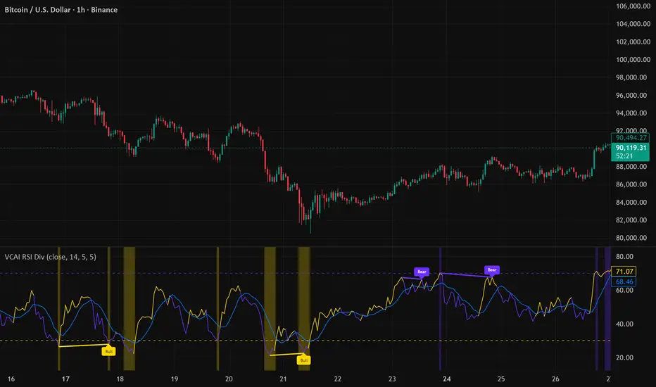
VCAI RSI Divergence +VCAI RSI Divergence+ is an RSI that shows trend, momentum, and divergence using V-CoresAI colour logic instead of a single white line.
What it shows:
Yellow RSI line → bullish momentum (RSI above its MA; buy-side pressure in control)
Purple RSI line → bearish momentum (RSI below its MA; sell-side pressure in control)
Thin blue line → fast RSI moving average that drives the colour flips
Dashed 70/30 lines → classic OB/OS zones
Background bands → soft purple in OB, soft yellow in OS to mark exhaustion areas
How to read it:
Yellow & rising → momentum shifting bullish; pullbacks into yellow OS band can be accumulation zones
Purple & falling → momentum shifting bearish; pushes into purple OB band can be distribution/sell zones
Hard colour flips (yellow ↔ purple) mark trend regime changes, not minor RSI noise
Divergence mode (on/off)
The divergence engine scans RSI and price pivot structure:
Bullish divergence (yellow) → price lower low + RSI higher low
Bearish divergence (purple) → price higher high + RSI lower high
Lines and tags appear only where a meaningful disagreement between price and RSI exists, giving early context for potential reversals or fade setups.
Together, the momentum colours + optional divergence mapping give a far clearer market read than a standard RSI, with zero clutter and no guesswork.
Open Interest Z-Score [BackQuant]Open Interest Z-Score
A standardized pressure gauge for futures positioning that turns multi venue open interest into a Z score, so you can see how extreme current positioning is relative to its own history and where leverage is stretched, decompressing, or quietly re loading.
What this is
This indicator builds a single synthetic open interest series by aggregating futures OI across major derivatives venues, then standardises that aggregated OI into a rolling Z score. Instead of looking at raw OI or a simple change, you get a normalized signal that says "how many standard deviations away from normal is positioning right now", with optional smoothing, reference bands, and divergence detection against price.
You can render the Z score in several plotting modes:
Line for a clean, classic oscillator.
Colored line that encodes both sign and momentum of OI Z.
Oscillator histogram that makes impulses and compressions obvious.
The script also includes:
Aggregated open interest across Binance, Bybit, OKX, Bitget, Kraken, HTX, and Deribit, using multiple contract suffixes where applicable.
Choice of OI units, either coin based or converted to USD notional.
Standard deviation reference lines and adaptive extreme bands.
A flexible smoothing layer with multiple moving average types.
Automatic detection of regular and hidden divergences between price and OI Z.
Alerts for zero line and ±2 sigma crosses.
Aggregated open interest source
At the core is the same multi venue OI aggregation engine as in the OI RSI tool, adapted from NoveltyTrade's work and extended for this use case. The indicator:
Anchors on the current chart symbol and its base currency.
Loops over a set of exchanges, gated by user toggles:
Binance.
Bybit.
OKX.
Bitget.
Kraken.
HTX.
Deribit.
For each exchange, loops over several contract suffixes such as USDT.P, USD.P, USDC.P, USD.PM to cover the common perp and margin styles.
Requests OI candles for each exchange plus suffix pair into a small custom OI type that carries open, high, low and close of open interest.
Converts each OI stream into a common unit via the sw method:
In COIN mode, OI is normalized relative to the coin.
In USD mode, OI is scaled by price to approximate notional.
Exchange specific scaling factors are applied where needed to match contract multipliers.
Accumulates all valid OI candles into a single combined OI "candle" by summing open, high, low and close across venues.
The result is oiClose , a synthetic close for aggregated OI that represents cross venue positioning. If there is no valid OI data for the symbol after this process, the script throws a clear runtime error so you know the market is unsupported rather than quietly plotting nonsense.
How the Z score is computed
Once the aggregated OI close is available, the indicator computes a rolling Z score over a configurable lookback:
Define subject as the aggregated OI close.
Compute a rolling mean of this subject with EMA over Z Score Lookback Period .
Compute a rolling standard deviation over the same length.
Subtract the mean from the current OI and divide by the standard deviation.
This gives a raw Z score:
oi_z_raw = (subject − mean) ÷ stdDev .
Instead of plotting this raw value directly, the script passes it through a smoothing layer:
You pick a Smoothing Type and Smoothing Period .
Choices include SMA, HMA, EMA, WMA, DEMA, RMA, linear regression, ALMA, TEMA, and T3.
The helper ma function applies the chosen smoother to the raw Z score.
The result is oi_z , a smoothed Z score of aggregated open interest. A separate EMA with EMA Period is then applied on oi_z to create a signal line ma that can be used for crossovers and trend reads.
Plotting modes
The Plotting Type input controls how this Z score is rendered:
1) Line
In line mode:
The smoothed OI Z score is plotted as a single line using Base Line Color .
The EMA overlay is optionally plotted if Show EMA is enabled.
This is the cleanest view when you want to treat OI Z like a standard oscillator, watching for zero line crosses, swings, and divergences.
2) Colored Line
Colored line mode adds conditional color logic to the Z score:
If the Z score is above zero and rising, it is bright green, representing positive and strengthening positioning pressure.
If the Z score is above zero and falling, it shifts to a cooler cyan, representing positive but weakening pressure.
If the Z score is below zero and falling, it is bright red, representing negative and strengthening pressure (growing net de risking or shorting).
If the Z score is below zero and rising, it is dark red, representing negative but recovering pressure.
This mapping makes it easy to see not only whether OI is above or below its historical mean, but also whether that deviation is intensifying or fading.
3) Oscillator
Oscillator mode turns the Z score into a histogram:
The smoothed Z score is plotted as vertical columns around zero.
Column colors use the same conditional palette as colored line mode, based on sign and change direction.
The histogram base is zero, so bars extend up into positive Z and down into negative Z.
Oscillator mode is useful when you care about impulses in positioning, for example sharp jumps into positive Z that coincide with fast builds in leverage, or deep spikes into negative Z that show aggressive flushes.
4) None
If you only want reference lines, extreme bands, divergences, or alerts without the base oscillator, you can set plotting to None and keep the rest of the tooling active.
The EMA overlay respects plotting mode and only appears when a visible Z score line or histogram is present.
Reference lines and standard deviation levels
The Select Reference Lines input offers two styles:
Standard Deviation Levels
Plots small markers at zero.
Draws thin horizontal lines at +1, +2, −1 and −2 Z.
Acts like a classic Z score ladder, zero as mean, ±1 as normal band, ±2 as outer band.
This mode is ideal if you want a textbook statistical framing, using ±1 and ±2 sigma as standard levels for "normal" versus "extended" positioning.
Extreme Bands
Extreme bands build on the same ±1 and ±2 lines, then add:
Upper outer band between +3 and +4 Z.
Lower outer band between −3 and −4 Z.
Dynamic fill colors inside these bands:
If the Z score is positive, the upper band fill turns red with an alpha that scales with the magnitude of |Z|, capped at a chosen max strength. Stronger deviations towards +4 produce more opaque red fills.
If the Z score is negative, the lower band fill turns green with the same adaptive alpha logic, highlighting deep negative deviations.
Opposite side bands remain a faint neutral white when not in use, so they still provide structural context without shouting.
This creates a visual "danger zone" for position crowding. When the Z score enters these outer bands, open interest is many standard deviations away from its mean and you are dealing with rare but highly loaded positioning states.
Z score as a positioning pressure gauge
Because this is a Z score of aggregated open interest, it measures how unusual current positioning is relative to its own recent history, not just whether OI is rising or falling:
Z near zero means total OI is roughly in line with normal conditions for your lookback window.
Positive Z means OI is above its recent mean. The further above zero, the more "crowded" or extended positioning is.
Negative Z means OI is below its recent mean. Deep negatives often mark post flush environments where leverage has been cleared and the market is under positioned.
The smoothing options help control how much noise you want in the signal:
Short Z score lookback and short smoothing will react quickly, suited for short term traders watching intraday positioning shocks.
Longer Z score lookback with smoother MA types (EMA, RMA, T3) give a slower, more structural view of where the crowd sits over days to weeks.
Divergences between price and OI Z
The indicator includes automatic divergence detection on the Z score versus price, using pivot highs and lows:
You configure Pivot Lookback Left and Pivot Lookback Right to control swing sensitivity.
Pivots are detected on the OI Z series.
For each eligible pivot, the script compares OI Z and price at the last two pivots.
It looks for four patterns:
Regular Bullish – price makes a lower low, OI Z makes a higher low. This can indicate selling exhaustion in positioning even as price washes out. These are marked with a line and a label "ℝ" below the oscillator, in the bullish color.
Hidden Bullish – price makes a higher low, OI Z makes a lower low. This suggests continuation potential where price holds up while positioning resets. Marked with "ℍ" in the bullish color.
Regular Bearish – price makes a higher high, OI Z makes a lower high. This is a classic warning sign of trend exhaustion, where price pushes higher while OI Z fails to confirm. Marked with "ℝ" in the bearish color.
Hidden Bearish – price makes a lower high, OI Z makes a higher high. This is often seen in pullbacks within downtrends, where price retraces but positioning stretches again in the direction of the prevailing move. Marked with "ℍ" in the bearish color.
Each divergence type can be toggled globally via Show Detected Divergences . Internally, the script restricts how far back it will connect pivots, so you do not get stray signals linking very old structures to current bars.
Trading applications
Crowding and squeeze risk
Z scores are a natural way to talk about crowding:
High positive Z in aggregated OI means the market is running high leverage compared to its own norm. If price is also extended, the risk of a squeeze or sharp unwind rises.
Deep negative Z means leverage has been cleaned out. While it can be painful to sit through, this environment often sets up cleaner new trends, since there is less one sided positioning to unwind.
The extreme bands at ±3 to ±4 highlight the rare states where crowding is most intense. You can treat these events as regime markers rather than day to day noise.
Trend confirmation and fade selection
Combine Z score with price and trend:
Bull trends with positive and rising Z are supported by fresh leverage, usually more persistent.
Bull trends with flat or falling Z while price keeps grinding up can be more fragile. Divergences and extreme bands can help identify which edges you do not want to fade and which you might.
In downtrends, deep negative Z that stays pinned can mean persistent de risking. Once the Z score starts to mean revert back toward zero, it can mark the early stages of stabilization.
Event and liquidation context
Around major events, you often see:
Rapid spikes in Z as traders rush to position.
Reversal and overshoot as liquidations and forced de risking clear the book.
A move from positive extremes through zero into negative extremes as the market transitions from crowded to under exposed.
The Z score makes that path obvious, especially in oscillator mode, where you see a block of high positive bars before the crash, then a slab of deep negative bars after the flush.
Settings overview
Z Score group
Plotting Type – None, Line, Colored Line, Oscillator.
Z Score Lookback Period – window used for mean and standard deviation on aggregated OI.
Smoothing Type – SMA, HMA, EMA, WMA, DEMA, RMA, linear regression, ALMA, TEMA or T3.
Smoothing Period – length for the selected moving average on the raw Z score.
Moving Average group
Show EMA – toggle EMA overlay on Z score.
EMA Period – EMA length for the signal line.
EMA Color – color of the EMA line.
Thresholds and Reference Lines group
Select Reference Lines – None, Standard Deviation Levels, Extreme Bands.
Standard deviation lines at 0, ±1, ±2 appear in both modes.
Extreme bands add filled zones at ±3 to ±4 with adaptive opacity tied to |Z|.
Extra Plotting and UI
Base Line Color – default color for the simple line mode.
Line Width – thickness of the oscillator line.
Positive Color – positive or bullish condition color.
Negative Color – negative or bearish condition color.
Divergences group
Show Detected Divergences – master toggle for divergence plotting.
Pivot Lookback Left and Pivot Lookback Right – how many bars left and right to define a pivot, controlling divergence sensitivity.
Open Interest Source group
OI Units – COIN or USD.
Exchange toggles for Binance, Bybit, OKX, Bitget, Kraken, HTX, Deribit.
Internally, all enabled exchanges and contract suffixes are aggregated into one synthetic OI series.
Alerts included
The indicator defines alert conditions for several key events:
OI Z Score Positive – Z crosses above zero, aggregated OI moves from below mean to above mean.
OI Z Score Negative – Z crosses below zero, aggregated OI moves from above mean to below mean.
OI Z Score Enters +2σ – Z enters the +2 band and above, marking extended positive positioning.
OI Z Score Enters −2σ – Z enters the −2 band and below, marking extended negative positioning.
Tie these into your strategy to be notified when leverage moves from normal to extended states.
Notes
This indicator does not rely on price based oscillators. It is a statistical lens on cross venue open interest, which makes it a complementary tool rather than a replacement for your existing price or volume signals. Use it to:
Quantify how unusual current futures positioning is compared to recent history.
Identify crowded leverage phases that can fuel squeezes.
Spot structural divergences between price and positioning.
Frame risk and opportunity around events and regime shifts.
It is not a complete trading system. Combine it with your own entries, exits and risk rules to get the most out of what the Z score is telling you about positioning pressure under the hood of the market.
